Jul 20, 2009 - Clustering of ordered data sets is a common problem faced in many pattern ... similarity between curves using scale-space distance. Shape similarity or ... 4b-d shows 3d curves formed from pairs of variational patterns shown in Figure 4a. ... where there are zero-crossings of the second derivative. Salient.
Order-preserving Clustering and Its Application to Gene Expression Data Tanveer Syeda-Mahmood IBM Almaden Research Center 650 Harry Road, San Jose, CA 95120
ABSTRACT Clustering of ordered data sets is a common problem faced in many pattern recognition tasks. Existing clustering methods either fail to capture the data or use restrictive models such as HMMs or AR models to model the data. In this paper, we present a general order-preserving clustering algorithm that allows arbitrary patterns of data evolution by representing each ordered set as a curve. Clustering of the data then reduces to grouping curves based on shape similarity. We develop a novel measure of shape similarity between curves using scale-space distance. Shape similarity or dis-similarity is judged by composing higherdimensional curves from constituent curves and noting the additional twists and turns in such curves that can be attributed to shape differences. An algorithm analogous to K-means clustering is then developed that uses prototypical curves for representing clusters. Results are demonstrated on ordered gene expression data sets obtained from gene chips.
1. Introduction Clustering of ordered data sets is a problem that occurs frequently in many pattern recognition tasks. A case in point is gene expression data, whose analysis has become popular with the advent of gene chips [1]. Clustering groups of genes or samples by analyzing their variational patterns with respect to time, dosage, patient age, etc. reveals more information about functionally similar genes than is possible with the clustering of their intensity values alone. Existing methods of clustering ordered data sets either fail to capture the order present in the data or use restrictive data models. Algorithms such as hierarchical clustering, neural clustering, SOMs, Gaussian mixture models, and graph-theoretic models [1, 7, 3, 6, 8] project the data as points in multi-dimensional space and use a distance metric such as the Euclidean distance, to measure similarity. Projecting the data as points in a multidimensional space inherently loses the order, so that a permutation of data points along the ordering dimension will not materially affect the distance. This can give erroneous result in clustering as shown in Figure 1, which shows 4 ordered data sets belonging to a single cluster. Some of the values in samples have been permuted in these data sets.
primarily suitable for modeling statistical time dependencies, and tend to be less sensitive to precise variations in the pattern of expression, leading to clusters that are not very compact. Figure 3 shows a representative cluster using AR modeling where the lack of compactness is apparent [6]. In the general case, when the measurement dimension is discrete, as in the case of patient samples, explicit dependency modeling may not even be possible.
Figure 2:Illustration of spread in the cluster using statistical modeling methods. Taken from [6]. In this paper, we present an approach that models the variational patterns as shapes to exploit the order present in the measurement dimension. Specifically, we represent a variational pattern as a curve and form a distance metric using a shape dis-similarity measure. Curves allow the dis-similarity between ordered data sets to be highlighted as can be seen from Figure 3 which shows the same data set of Figure 1 now approximated through curves.
Figure 3: Illustration of representing ordered data sets as curves. The rest of the paper describes how representing ordered data sets as curves allows a shape-based pattern recognition approach to clustering. It is organized as follows. In Section 2, we present a novel approach to measuring shape dis-similarity. In Section 3, we present the algorithm for clustering using mean shapes. Finally, in Section 4 & 5, we discuss the application of orderpreserving clustering to gene expression data sets and present results of shape-based clustering.
2. Capturing shape similarity Figure 1: Illustration of the importance of using order in data sets. Available methods for modeling the order in the data use restrictive parametric data models such as hidden Markov models [5] and autoregressive models [6]. These descriptions are
Given two 2d curves (g1(t),t) and (g2(t),t), let (G(t),t) = (g1(t),g2(t),t) be a 3d curve formed by projecting the two curves in 3-space (g1,g2,t). If g1 and g2 are similar in shape, the 3d curve is similar in shape to the individual constituent curves. However, if g1 and g2 differ in shape, the 3d curve depicts relatively large amounts of sharp twists, bends and turns over and
Proceedings of the 17th International Conference on Pattern Recognition (ICPR’04) 1051-4651/04 $ 20.00 IEEE Authorized licensed use limited to: KnowledgeGate from IBM Market Insights. Downloaded on July 20, 2009 at 18:12 from IEEE Xplore. Restrictions apply.
above the changes present in the component curves. Furthermore, these changes occur precisely at points where the pattern differs in the constituent curves, thus preserving inherently the order present in the variational pattern. Figure 4b-d shows 3d curves formed from pairs of variational patterns shown in Figure 4a. As can be seen, when the component curves are similar (for ORFs 18srRnaa and 18srRnac), their corresponding 3d curve (Figure 4b) shows similar changes as in the original curves. On the other hand, when two dissimilar signals are composed (18srRnaa and 18srRnab) as in Figure 4c or profiles 18srRnab and 18srRnac as shown in Figure 4d, the sharp bends and twists are apparent in the 3d curve. In fact, the sharpness of turn is proportional to the mismatch between the two component curves from which the 3d curve is derived. Thus by comparing the sharpness of bends in the 3d curve to the underlying shape of the component curves at corresponding points, we can obtain a measure of similarity between the two curves. This idea can be generalized for comparing multiple curves simultaneously by projecting n constituent curves into an n+1dimensional space and forming an n+1-dimensional curve.
(a)
For multi-dimensional curves, the above formula reduces to making the determinant of the Hessian to be zero. The original inflection points can then be recovered from negative-going zerocrossings of the second derivative. Thus if we look for places where there is a change of sign in the second derivative of the signal as a function of scale, the resulting 2d image looks as shown in Figure 5b. Here the zero-crossing contours are the contours of the colored regions. In particular, the negative-going zero-crossings are the contours of the red to blue transition regions (light-to-dark -in-gray image renderings). This is the curvature scale-space as described in [10, 4]. In particular, it can be shown that in the case of Gaussian smoothing, the zerocrossing contours are always closed at the bottom (higher scale) and open at the top (U shaped curves). Also, the zero-crossings shift with increasing scale, so that the exact location of a zerocrossing is found by starting from the peak of a contour and tracking the contour down to its finest scale location as described in [10]. The resulting representation is called the scale-space signal, and describes the location of sharp change points in the curve. In particular, the intensity at a point in a scale-space signal is the highest scale at which the change disappears. Thus sharper changes are reflected as high intensity points in the curve. Figure 5c shows the scale-space signal for the original curve in Figure 5a.
(b)
(a)
(b)
( c) (d) Figure 4: Illustration of measurement of shape dis-similarity.
2.1 Measuring shape similarity Our shape similarity measure captures sharp changes in the projected higher-dimensional curve and the associated constituent curves. Change points on curves are inflection points i.e. places where there are zero-crossings of the second derivative. Salient change points are those that are perceptually important, i.e., changes that are preserved even after multiple levels of smoothing. To detect the salient changes, we use scale-space analysis. Specifically, we form a continuous representation by successively smoothing a curve C(t) (projected or constituent) using a kernel (Gaussian kernel used) g (t , σ ) , so that we have ∞
Cˆ (t , σ ) = C (t ) *g (t , σ ) = ³ C (u ) −∞
1
σ 2π
e
−
( t −u ) 2 2σ 2
du (1)
The inflection points are locations of the zero-crossings of the second derivative, i.e., where
∂ Cˆ =0 ∂t 2 2
(2)
(c) Figure 5: Illustration of scale-space signal. (a) Original signal. (b) Its scale-space representation using Gaussian filters. (c) Scalespace signal.
2.2 Scale-space similarity metric Using the scale-space signals, the distance between two curves g1(t), and g2(t) is given by the following scale-space distance T
D( g1, g 2) = ¦ ( I C (i ) − i =1
( I 1 (i ) + I 2 (i )) 2 ) 2
Proceedings of the 17th International Conference on Pattern Recognition (ICPR’04) 1051-4651/04 $ 20.00 IEEE Authorized licensed use limited to: KnowledgeGate from IBM Market Insights. Downloaded on July 20, 2009 at 18:12 from IEEE Xplore. Restrictions apply.
where
I C (i ), I 1 (i ), I 2 (i )
are the scale-space signals of the
individual and combined curves respectively. This similarity measure remains a metric, since it can be interpreted as the Euclidean distance between the transformed curves in scale-space. Since the scale-space curves for multi-dimensional curves are also one-dimensional, the above distance metric can be used to compute the similarity between multi-dimensional curves and one-dimensional curves, two multi-dimensional curves, etc. This will be found useful in clustering the curves as discussed next.
3. Order-preserving clustering Once a shape matching distance metric is chosen, it can be used to substitute a distance metric used in any clustering algorithm to obtain various clustering schemes using curve shapes. In this paper, we focus on adapting the k-means clustering. While this is an older algorithm, the clusters produced have some desirable properties if proper initialization can be insured, and fast convergence can be obtained. Analogous to the concept of centroids, we use a mean shape, i.e., a multi-dimensional curve formed from the individual curves in the group to serve as a prototype for the cluster. Following the K-means algorithm, we proceed to do the clustering in 3 steps, namely, (1) initial prototype selection, (2) classification of curves, and (3) recomputation of the prototypes. Steps 2 and 3 are repeated until convergence is reached (when the prototypes do not change much). Different methods of initial selection of centroids can be used. Here we use the maximum scale-space distance between a randomly selected curve and all other curves, to assemble initial cluster prototypes. That is, K curves whose distance to one another attribute is greater than 0.9 * maximum scale-space distance, are retained as the initial K prototypes. In the classification step, the minimum scale-space distance between a curve and all K prototypes is used to assign a curve to the corresponding cluster. The multi-dimensional curve formed from the curves in a cluster becomes the new prototype for the next iteration. The complexity of the algorithm remains O(nK) for initialization of K prototypes for the n-element dataset, and O(mnK) for m iterations of data classification and O(mn) for recomputation of prototypes.
for experiments was the cell cycle data from Spellman et al [9] recording the expression of 6600 ORFs (some of which are genes) in the yeast genome. This dataset was assembled by Spellman et al.[9] who had found that several genes of the yeast genome are regulated by different phases of the mitotic cell-cycle using careful lab experiments. The data is available from Stanford (http://cellcycle-www.stanford.edu)[2] and depicts expression of genes against 17 experimental conditions (in this case, 17 time points). Modeling expression patterns are curves can also handle this case where the dependency between samples is based on time. We chose this data set as it has ground truth clusters defined where the clusters correspond to genes that are regulated by the same phase of the cell cycle. First, we illustrate the nature of clusters formed using the scalespace distance metric. Figure 6 shows three clusters obtained from the above data set, depicting a correct grouping of functionally related genes. It can also be seen that the clusters are compact and perceptually meaningful with co-regulation patterns clearly emerging, even though the scale of variation is considerably different within a cluster.
(a)
(b)
4. Application to gene expression data The above algorithm for order-preserving clustering was applied to the problem of clustering gene expression profiles to determine functionally similar genes. The data for clustering came from gene chips that record the expression of genes under several conditions and present it as a two-dimensional array of data where the rows represent genes and columns represent experimental conditions, samples, time, etc. Given a database of gene curves, the scalespace signals are derived for each of the curves. Scale-space signals of higher-dimensional curves are formed during the iteration steps of clustering as cluster prototypes are assembled. The result is an indexed database with the prototype curves per cluster serving as indexes. Given a new gene curve as a query, the system retrieves matching prototypes from clusters and lists the constituent genes in a cluster along with links to their associated information in a public database to allow scientists to infer functional similarity of a newly discovered gene.
5. Results We now present results to illustrate the utility of modeling curves as shapes in clustering gene expression data. The database used
(c ) Figure 6: Illustration of results of clustering using scale-space distance. (a)- (c) Three representative clusters formed from the gene expression data set described in text. Next, we compare clustering using scale-space distance and Euclidean distance for different choices of the number of clusters. The algorithm for initialization of centroids remains the same in both cases, using the farthest distance between a pair of genes as the seed distance for cluster separation. The results are tabulated in Table 1. Here Column 1 indicates the choice of K, column 2 & 3 indicate the number of members in corresponding clusters for the 10 largest clusters, and the percentage overlap between the corresponding clusters in the Euclidean distance case. The corresponding clusters are based on the highest amount of overlap. From this, we can infer that the two methods produce different cluster distributions. Next, in Column 4 and 5, we list the average intra-cluster compactness for the two cases as the ratio of the average distance to the maximum distance between pairs of
Proceedings of the 17th International Conference on Pattern Recognition (ICPR’04) 1051-4651/04 $ 20.00 IEEE Authorized licensed use limited to: KnowledgeGate from IBM Market Insights. Downloaded on July 20, 2009 at 18:12 from IEEE Xplore. Restrictions apply.
curves for the two choices of distance metrics. As expected, the cluster-compactness increases with the number of clusters. To compare the performance of both metrics for clustering against the ground truth data, we repeated clustering on a smaller data set consisting of 104 cell-cycle regulated genes that have already been manually clustered into functionally similar groups based on biological verification of their cell-cycle co-regulation patterns.
These genes are listed in Table 4 Column 3. We ran the clustering algorithms on the reduced data set consisting of 104 genes isolated above. The percentage overlap with the ground truth clusters for the same value of K is recorded for both clustering methods, and is shown in Column 4 and 5 of Table 2. As can be seen, the scale-space distance-based metric is more effective in grouping genes known to be functionally similar.
Table 1: Illustration of clustering using scale-space and Euclidean distance.
Table 2: Illustration of the accuracy of clustering using scale-space distance.
6. Conclusions In this paper, we have introduced a new pattern recognition-based method for order-preserving clustering. The scale-space distance has been shown to be effective in capturing shape similarity in curves thus giving rise to perceptually meaningful clusters while still preserving the order in the data set. REFERENCES [1] Y. Barash and N. Friedman. Context-specific Bayesian clustering for gene expression data. In Research in Computational Molecular Biology, pages 12-21, 2000. [2] R.J. Cho et al. A genome-wide transcriptional analysis of the mitotic cell cycle. Mol. Cell., 2:65-73, 1998. [3] Z-B. Joseph, D. Gifford, and T. Jaakkola. A new approach to analyzing gene expression time series. In Proc. RECOMB, pages 326{327, 2002. [4] T. Lindeberg. Detecting salient blob-like image structures and their scales with a scale-space primal sketch: A method for focus of attention. International Journal of Computer Vision, 3(11):283318, 1993.
[5] T. Oates et al. Clustering time series with hidden Markov models and dynamic time warping. In Proceedings of the IJCAI99 Workshop on Reinforcement Learning, 1999. [6] M.F. Ramoni et al. Cluster analysis of gene expression dynamics. Proc. National Acad. Sci. A, 99:9121{9126, 2002. [7] A. Schliep et al. Using hidden Markov models to analyze gene expression time course data. In Proceedings of the 8th Intl. Conference on Intelligent Systems for Molecular Biology (ISMB) 2003, pages 255{263, 2003. [8] R. Shamir and R. Sharan. Click: A clustering algorithm for gene expression analysis. In Proceedings of the 8th Intl. Conference on Intelligent Systems for Molecular Biology (ISMB) 2000, pages 724-726, 2000. [9] P. Spellman et al. Comprehensive identification of cell cycleregulated genes of the yeast Saccharomyces Cerevisiae by microarray hybridization. Molecular Biology of Cell, 9:3273{3297, 1998. [10] A. Witkin. Scale space filtering: A new approach to multiscale description. In Proceedings Int. Joint. Conf. Artif. Intell., 1984.
Proceedings of the 17th International Conference on Pattern Recognition (ICPR’04) 1051-4651/04 $ 20.00 IEEE Authorized licensed use limited to: KnowledgeGate from IBM Market Insights. Downloaded on July 20, 2009 at 18:12 from IEEE Xplore. Restrictions apply.