Journal of Advances in Computer Research Quarterly ISSN: 2008-6148 Sari Branch, Islamic Azad University, Sari, I.R.Iran (Vol. 5, No. 1, February 2014), Pages: 29-42 www.jacr.iausari.ac.ir
Order reduction by minimizing integral square error and H∞ norm of error Hasan Nasiri Soloklo1* and Malihe Maghfoori Farsangi2 1. Department of Electrical Engineering, Firoozkooh Branch, Islamic Azad university, firoozkooh, Iran 2. Electrical Engineering Department, Shahid Bahonar University of Kerman, Kerman, Iran
[email protected];
[email protected] Received: 2013/08/17;
Accepted: 2013/9/30
Abstract In this paper, a new alternative method for order reduction of high order systems is presented based on optimization of multi objective fitness function by using Harmony Search algorithm. At first, step response of full order system is obtained as a vector, then, a suitable fixed structure considered for model order reduction which order of original system is bigger than fixed structure model. Parameters of model order reduction are determined by minimizing the multi objective fitness function where the fitness function is conducted with integral square error and H∞ norm of error. The harmony search algorithm is applied for minimizing the multi objective fitness function. To assure the stability, the Routh criterion is applied for specifying the stability conditions. This stability condition is considered as constraints in optimization problem. To present the accuracy y of the proposed method, three test systems are reduced. The obtained results show that the proposed approach performs very well. Keywords: Harmony search, model reduction, Routh criterion, H∞ norm, Integral square error
1. Introduction Since, the most systems are large scale and the mathematical models for analysis are high order and complicated, therefore, accurate analysis and design of such high order systems are very difficult and time consuming. Model order reduction is the most efficient approach that is investigated by researchers and engineers. In this approach, high order system is approximated with reduced order model such that the most characteristics high order system is retained in the reduced model. Model order reduction is presented by Davison [1] in 1966, for the first time. Then Chidambara investigated several improvement for Davison approach in 1967 and 1969 [2]-[3]. Optimal model order reduction of high order system is considered by Wilson in 1970. Wilson used optimization method based on minimization of Integral Square Error (ISE) that error is considered as difference between impulse response of full order model and reduced order model [4]-[5]. Friedland and Hutton in [6] used Routh approach for high frequency approximation, then this method is improved by Langholz and Femines in 1978 [7].
29
Order reduction by minimizing integral …
H. Nasiri Soloklo, M. Maghfoori Farsangi
Then El-Attar and Vidyasagur presented a method by minimizing L1 and L∞ [8]. In the early 1980s, Eittelberg [9] and Obineta [10] obtained the reduced model based on minimizing error equation. In 1981 [11], Moore considered the controllability and observability of the states in model order reduction problems. The suggested approach suffered from steady state errors but the stability of the reduced model was assured if the original system was also stable. After Moore, Glover reduced the high order models with a similar concept, called the optimal Hankel approximation [12]. Furthermore, the concepts of H2, L2 and L∞ were used in model reduction [13]-[15]. In 1995, Feldman and Fround presented an approach for model order reduction based on Pade approximation [16]. In the recent decade, the evolutionary algorithms such as Genetic Algorithm (GA), Particle Swarm Optimization (PSO) and Harmony Search (HS) algorithm are used widely for model reduction of high order systems [17]-[19]. In these approaches, the reduced order model's parameters are achieved by minimizing a fitness function, which is often Integral Square Error (ISE) [20]-[21]. In this paper, a new alternative method is proposed for model order reduction based on minimizing the multi objective fitness function. In this method, the step response of full order system is achieved. A desire fixed structure for reduced order model is considered and a set of parameters are defined, those values determine the reduced order system. These unknown parameters are determined using Harmony Search (HS) algorithm by minimizing the multi objective fitness function that the fitness function is integral square error (ISE) plus H ∞ norm of error and this error is defined as difference between step response of full order model and reduced order model. To satisfy the stability, Routh criterion is utilized as it is used in [22] where, it states in optimization problem as constraints and subsequently, optimization problem converted to a constrained optimization problem. To show the accuracy of the proposed method, three test systems are reduced by the proposed method and compared with some other methods of model order reduction. The paper is organized as follows: to make a proper background, the HS is explained in Section 2. The proposed method is explained in Section 3. The capability of the proposed approach is shown in Section 4 through three test systems and the paper is concluded in Section 5. 2. Overview of HS algorithm The HS is based on natural musical performance a process that searches for a perfect state of harmony. In general, the HS algorithm works as follows [24]-[25]: Step1. Initialization: Initial population is produced randomly within the range of the boundaries of the decision variables. The optimization problem can be defined as: Minimize f (x ) subject to x iL < x i < x iU (i = 1, 2, , N ) where x iL and x iU are the lower and upper bounds for decision variables. The HS algorithm parameters are also specified in this step. They are the harmony memory size (HMS) or the number of solution vectors in harmony memory, harmony memory considering rate (HMCR), distance bandwidth (bw), pitch adjusting rate (PAR), and the number of improvisations (K), or stopping criterion. K is the same as the total number of function evaluations.
30
Journal of Advances in Computer Research
(Vol. 5, No. 1, February 2014) 29-42
Step2. Initialize the harmony memory (HM). The harmony memory is a memory location where all the solution vectors (sets of decision variables) are stored. The initial harmony memory is randomly generated in the region [ x iL , x iU ] (i = 1, 2, , N ) . This is done based on the following equation: x ij = x iL + rand ( ) × ( x iU − x iL )
j = 1,2,, HMS
(1)
where rand ( ) is a random number from a uniform distribution on [0,1]. Step3. Improvise a new harmony from the harmony memory. Generating a new harmony x inew is called improvisation where it is based on 3 rules: memory consideration, pitch adjustment and random selection. First of all, a uniform random number R is generated in the range [0, 1]. If R is less than HMCR, the decision variable x inew is generated by the memory consideration; otherwise, x inew is obtained by a random selection. Then, each decision variable x inew will undergo a pitch adjustment with a probability of PAR if it is produced by the memory consideration. The pitch adjustment rule is given as follows:
x inew = x inew ± R ×bw
(2)
Step4. Update harmony memory. After a new harmony vector x new is generated, the harmony memory will be updated. If the fitness of the improvised harmony vector new x new = x 1new , x 2new , , x N is better than that of the worst harmony, the worst harmony
(
)
in the HM will be replaced with x new and become a new member of the HM. Step5. Repeat steps 3 and 4 until the stopping criterion (maximum number of improvisations K) is met. The optimum design algorithm using HS is sketched basically as shown in Fig. 1. Initialize HS parameters
Initialize HM
Improvise a new harmony
Update HM
NO
Termination criteria
YES
Program terminated
Figure 1. The basic flowchart diagram for HS algorithm.
31
Order reduction by minimizing integral …
H. Nasiri Soloklo, M. Maghfoori Farsangi
3. The Proposed method Consider a stable high order system, which presented by the transfer function of order n as follows: G (s ) =
a1s n −1 + a 2 s n − 2 + + a n s n + b1s n − 2 + b 2 s n − 2 + + b n
(3)
where a i and b i are known constants. The objective is obtaining a reduced model of order r which r is less than n such that the principle and most significant specification are retained in reduced order model. This reduced order model is offered as follows: G r (s ) =
c1s n −1 + c 2 s n − 2 + + c n s n + d 1s n − 2 + d 2 s n − 2 + + d n
(4)
where c i and d i are unknown constants that should be determined. For specifying the unknown parameters and consequently reduced order model, first, the step response of full order system is obtained. Then a desire fixed structure is considered for reduced order model. Harmony search algorithm is used for determining the unknown constants by minimizing the fitness function. If y f and y r are step response of full order and reduced model in interval [ 0, t f ] respectively, then by minimizing the following fitness function using HS, the unknown parameters are obtained: ∗
J =
tf
∫(y
− y r ) dt + ( y f − y r ) 2
f
(5)
∞
0
Since the full order system in (3) is stable, thus the reduced order model must be stable. In other words, the proposed model must guarantee the stability. To this goal, the Routh criterion is applied as follows: The denominator of reduced order model, which is presented by (4) can be shown as below [22]:
s r + h1s r −1 + (h2 + h3 + ... + hr )s r −2 + h1(h3 + h4 + ... + hr )s r −3 + [h2 (h4 + h5 + ... + hr ) + h3 (h5 + h6 + ... + hr ) +
(6)
h4 (h6 + h7 + ... + hr ) + ... Which is constructed by taking the coefficients of the first two rows of the Routh array with the elements of its first column given by
1, h1 , h2 , h1h3 , h2 h4 , h1h3h5 ,..., h1+ k h3+ k ...hr −2 hr
(7)
where, k is equal to 1 for even r and k is equal to 0 for odd r. Comparing the entries of the first row with 1, d 2 , d 4 , and those of the second row with d 1 , d 3 , d 5 , the relations defined in (8) is obtained:
32
Journal of Advances in Computer Research
(Vol. 5, No. 1, February 2014) 29-42
d 1 = h1 d 2 = (h2 + h3 + ... + hr ) d 3 = h1 (h3 + h4 + ... + hr )
(8)
d r = (h1+ k h3+ k hr − 2 hr )
Substituting the above relations in reduced order model's denominator, (6) is achieved. Therefore, the necessary and sufficient condition for all the poles of the reduced system to be strictly in the left-half plane is h1 > 0 h2 > 0
(9)
hr > 0 and subsequently d1 > 0 d2 > 0
(10)
dr > 0
Thus, to have a stable reduced system, the parameters of reduced order model are determined by minimizing the (5) subject to (10). In other words, optimization problem in (5) is converted to constrained optimization problem as follows: min J =
tf
∫(y
− y r ) dt + ( y f − y r ) 2
f
∞
0
(11)
subject to d j > 0 for j = 1, , r
Minimizing the above fitness function by using harmony search algorithm, the reduced order model’s parameters are obtained so that the reduced model guarantees the stability. The reduced order model, which is obtained by this method retains the main and important characteristic of the original system such as maximum overshoot, steady state value and rise time. The proposed method can be summarized in the following steps: Step1: The step response of full order model is obtained. Step2: A desire fixed structure for reduced order model is considered as (4) where c i and d i are unknown parameters of reduced order model that are determined in following steps. Step3: HS is used to obtain the unknown parameters. The purpose of the optimization is to find the best parameters for G r ( s ) . Therefore, each harmony is a d dimensional vector in which d is c i + d i . Each harmony is a solution to G r and for each solution (harmony), the reduced order model is obtained. Each harmony in the 33
Order reduction by minimizing integral …
H. Nasiri Soloklo, M. Maghfoori Farsangi
population is evaluated using the objective function defined by (11) searching for the harmony associated with J best until the termination criteria is met. At this stage, the best parameters are given as parameters of reduced order model. 4. Simulation and Results In this section, three test systems are considered and then these systems are reduced by the proposed method to show the efficiency of the proposed method. The proposed method and other model reduction methods are implemented using MATLAB. A step by step procedure is given for test system 1. Test system 1: the first test system is a 9-order model that is considered by Mukherjee in [26] as follows: GOrg =
s 4 + 35s 3 + 291s 2 + 1093s + 1700 s 9 + 9s 8 + 66s 7 + 294s 6 + 1029s 5 + 2541s 4 + 4684s 3 + 5856s 2 + 4620s + 1700
(12)
The reduced-order model can be obtained by the following steps: Step1: the step response of the original order system (12) is obtained. Step2: an optimal fixed structure for reduced order model is considered as follows: G ISE + H inf =
c1s 2 + c 2 s + c 3 s + d 1s 2 + d 2 s + d 3
(13)
3
where c i and d i are unknown parameters that should be determined. Step 3: HS is applied to obtain the unknown parameters in (13). Since, the aim of the optimization is to find the best parameters for G r ( s ) , therefore, each harmony is a d dimensional vector in which d = 6 . The HMS is selected to be 10, HMCR and evaluation number is set to be 0.9 and 1000, respectively. Each harmony is a solution to G r ( s ) and for each solution (harmony), the step response of reduced order model is obtained. Each harmony is evaluated using the fitness function defined by (11) searching for the best J until the termination criteria is met. At this stage, the best parameters are given for reduced order model where, the following reduced order model is obtained: G ISE + H inf =
0.7261s 2 − 2.8835s + 5.0391
(14)
s 3 + 4.5397s 2 + 7.5708s + 5.0391
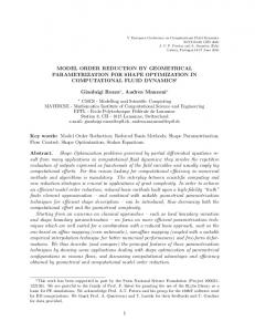
The step response of the full order system and that of the system with third-order reduced models are shown in Fig. 2.
34
Journal of Advances in Computer Research
(Vol. 5, No. 1, February 2014) 29-42
Step Response 1.2
1
Amplitude
0.8
0.6
0.4
0.2 Original system
0
ISE+Hinf -0.2
0
1
2
3
4
5
6
Time (sec)
Figure 2 . Step response of full order and reduced order model by the proposed method for test system
This figure shows that the obtained reduced order model is an adequate low-order model that maintains the specifications of full order model. Also, to show the efficiency of the proposed method, the step responses of the achieved reduced model are compared with those available in the literature. Figs. 3, shows the comparison of the results obtained with the proposed method by Mukherjee [26], Optimal Hankel norm approximation (HSV) [23] and Balanced Truncation (BT) [23], respectively.
35
Order reduction by minimizing integral …
H. Nasiri Soloklo, M. Maghfoori Farsangi
Step Response 1.2
1
Amplitude
0.8
0.6
0.4 Original system
0.2
ISE+Hinf Proposed by Mukherjee
0
BT HSV
-0.2
0
2
4
6
8
10
12
14
Time (sec)
Figure 3. Step response of full order and reduced order model by the proposed method and other conventional methods for test system 1.
Furthermore, the main characteristics of the reduced model by the proposed method such as steady state value, settling time and maximum overshoot are compared with those obtained by Mukherjee [26], HSV and BT where shown in Table 1. Also, integral square error (ISE) and the H ∞ norm of the error between the step responses of full order and reduced order models ( e = y f − y r ) are given in Table 1. It is clearly seen that the specifications of reduced order model that is achieved by the proposed method are close to the specifications of original system. Table 1- Comparison of methods for test system 1. Steady state 1
Over shoot (%) 0
Rise time (sec) 1.54
Settling time (sec) 3.36
1
0.9
1.81
1
0
BT method
1.1
HSV method
1.12
original system The proposed method (ISE+Hinf) Proposed by Mukherjee
-
Infinity norm of error -
3.67
0.0050
0.0541
2.02
4.32
0.0131
0.0867
0
2.11
6.62
0.0734
0.0959
0
1.93
6.11
0.1479
0.1207
36
ISE
Journal of Advances in Computer Research
(Vol. 5, No. 1, February 2014) 29-42
Also, the plot of e = y f − y r is shown in Fig. 4 for reduced systems. It can be seen from figure 4 that the obtained error by the proposed method in this paper is less than other methods. 0.14 0.12
Absolute of Error
0.1 0.08 0.06 ISE+Hinf Proposed by Mukherjee BT HSV
0.04 0.02 0
0
5
10
15
Time(sec)
Figure 4. The plot of e = y − y r for the full order and reduced systems by the proposed method and other methods for test system 1.
Test system 2: In [27], a procedure is presented to obtain a reduced order system by Routh-Pade approximation using Luus-Jaakola algorithm. To compare the proposed method in this paper with Luus-Jaakola algorithm, the system given in [27] is considered as follows: Gorg =
8s 2 + 6s + 2
(15)
s 3 + 4s 2 + 5s + 2
Based on the explanations given for test system 1, the obtained reduced system by the proposed method is as below: G ISE + H inf =
8.6531s + 5.0443
(16)
s + 4.0136s + 5.0493 2
The step response of the full order system and the obtained reduced model is shown in Fig. 5. In this figure, the responses of the system with second-order primary reduced models obtained by other methods such as BT method and HSV method and included for comparison. Also, the plot of e = y − y r is plotted for the reduced systems in Fig. 6.
37
Order reduction by minimizing integral …
H. Nasiri Soloklo, M. Maghfoori Farsangi
Step Response 2 Original system
1.8
ISE+Hinf Proposed by Singh
1.6
BT 1.4
HSV
Amplitude
1.2 1 0.8 0.6 0.4 0.2 0
0
1
2
3
4
5
6
7
8
9
Time (sec)
Figure 5. Step response of full order and reduced order model by the proposed method and other conventional methods for test system 2.
0.35 ISE+Hinf Proposed by Singh BT HSV
0.3
Absolute of Error
0.25 0.2 0.15 0.1 0.05 0
0
2
4
6
8
10 12 Time(sec)
14
16
18
20
Figure 6. The plot of e = y − y r for the full order and reduced systems by the proposed method and other methods for test system 2.
38
Journal of Advances in Computer Research
(Vol. 5, No. 1, February 2014) 29-42
The main characteristics of full order model and reduced models, which is obtained by the proposed method and other classic methods, are presented in Table 2. In addition, two error criteria such as ISE and H ∞ norm of error are calculated in Table 2. Table 2- Comparison of methods for test system 2. Steady state
Overshoot (%)
Rise time (sec)
Settling time (sec)
ISE
Infinity norm of error
original system The proposed method (ISE+Hinf) Proposed by Singh
1
86.5
0.129
6.74
-
-
0.999
87.9
0.118
2.63
0.0404
0.1320
1
66.1
0.13
1.71
0.1404
0.3425
BT method
0.836
123
0.103
3.15
0.3802
0.1635
HSV method
0.836
115
0.118
3.44
0.4043
0.1635
The comparison of the proposed method with those conventional model order reduction method indicates that the proposed method has a better performance. Test system 3: The system given in [28] by Parmar is the third system to be reduced. The system is as follows: G (s ) =
18s 7 + 514s 6 + 5928s 5 + 36380s 4 + 122664s 3 + 222088s 2 + 185760s + 40320 s + 36s 7 + 546s 6 + 4536s 5 + 22449s 4 + 67284s 3 + 118124s 2 + 109584s + 40320 8
(17)
Based on the explanations given for test system 1, the obtained reduced system by the proposed method is as follows: G( s) =
17.5s + 5.54 s + 7.16s + 5.5
(18)
2
The comparison of the proposed method with the proposed ones by Parmar and BT method and HSV method is shown in Figs. 7 and 8 and Table 3, which illustrate a better performance of the proposed method.
39
Order reduction by minimizing integral …
H. Nasiri Soloklo, M. Maghfoori Farsangi
Step Response 2.5 Original system ISE+Hinf Proposed by Parmar BT
2
HSV
A m p litu d e
1.5
1
0.5
0
0
1
2
3
4
5
6
7
8
9
Time (seconds)
Figure 7. Step response of full order and reduced order model by the proposed method and other conventional methods for test system 3. 0.35 ISE+Hinf Proposed by Parmar BT HSV
0.3
A b s o lu t e o f E rro r
0.25
0.2
0.15
0.1
0.05
0
0
5
10
15
Time(sec)
Figure 8. The plot of e = y − y r for the full order and reduced systems by the proposed method and other methods for test system 3. 40
Journal of Advances in Computer Research
(Vol. 5, No. 1, February 2014) 29-42
Table 3- Comparison of the methods for test system 3. Steady state
Overshoot (%)
Rise time (sec)
Settling time (sec)
ISE
Infinity norm of error
1
120
0.0569
4.82
-
-
1
121
0.0578
5.04
0.0016
0.0387
1
130
0.0439
4.4
0.0368
0.2668
BT
0.94
134
0.0529
5.97
0.0491
0.0595
HSV
0.944
132
0.0556
5.48
0.0483
0.0559
Original system The proposed method (ISE+Hinf) Proposed by Parmar
5. Conclusions In this paper, a method is investigated for model order reduction based on minimizing two errors criteria; Integral Square Error and H ∞ norm of error. In this method, reduced model parameters are determined by using harmony search algorithm. Routh array is used to determine the stability conditions. To present the accuracy and ability of the method, three test systems are reduced by the proposed method and compared with some conventional order reduction techniques. The obtained results show that the proposed approach has high accuracy respect to conventional order reduction methods. 6. References [1]. E. J. Davison, “A method for simplifying linear dynamic systems”, IEEE Trans. on Automatic Control, Vol. 11, 1996, pp. 93–101. [2]. M. R. Chidambara, “Further comments by M.R. Chidambara”, IEEE Trans. on Automatic Control, Vol. 1, 1967, pp. 799–800. [3]. M. R. Chidambara, “Two simple techniques for the simplification of large dynamic systems”, in Proc. JACC, 1969, pp. 669–674. [4]. D. A. Wilson, “Optimal solution of model reduction problem”, in Proc. Institute of Electrical Engineering, 1970, pp. 1161-1165. [5]. D. A. Wilson, “Model reduction for multivariable systems”, International Journal of Control, Vol. 20, 1974, pp. 57–64. [6]. M. Hutton and B. Friedland, “Routh approximations for reducing order of linear, time-invariant systems”, IEEE Trans. on Automatic Control, Vol. 20, No. 3, 1975, pp. 329–337. [7]. G. Langholz, and D. Feinmesser, “Model reduction by routh approximations”, Int. J. Syst. Sci., Vol. 9, No. 5, 1978, pp. 493-496. [8]. R. A. El-Attar and M. Vidyasagar, “Order reduction by L1 and L∞ Norm minimization”, IEEE Trans. on Automatic Control, Vol. 23, No. 4, 1978, pp. 731–734. [9]. E. Eitelberg, “Model reduction by minimizing the weighted equation error”, International Journal of Control, Vol. 34, No. 6, 1981, pp. 1113-1123. [10]. G. Obinata and H. Inooka, “Authors reply to comments on model reduction by minimizing the equation error”, IEEE Trans. on Automatic Control, Vol. 28, 1983, pp. 124–125.
41
Order reduction by minimizing integral …
H. Nasiri Soloklo, M. Maghfoori Farsangi
[11]. B. C. Moore, “Principal component analysis in linear systems: controllability, observability and model reduction”, IEEE Trans. on Automatic Control, Vol. 26, 1981, pp. 17–32. [12]. K. Glover, “All optimal hankel norm approximation of linear multivariable systems and their L∞ error bounds”, Int. J. Control, Vol. 39, 1984, pp. 1115-1193. [13]. L. Zhang and J. Lam, “On H2 model reduction of bilinear system” Automatica , Vol. 38, 2002, pp. 205–216. [14]. W. Krajewski, A. Lepschy, G. A. Mian and U. Viaro, “Optimality conditions in multivariable L2 model reduction,” Journal of the Franklin Institute, Vol. 330, No. 3, 1993, pp. 431–439. [15]. D. Kavranoglu and M. Bettayeb, “Characterization and computation of the solution to the optimal L∞ approximation problem,” IEEE Trans. on Automatic Control, Vol. 39, 1994, pp. 1899–1904. [16]. P. Feldman and R.W. Freund, “Efficient linear circuit analysis by Padé approximation via a Lanczos method”, IEEE Trans. Computer-Aided Des., Vol. 14, 1995, pp. 639-649. [17]. G. Parmer, R. Prasad and S. Mukherjee, “Order Reduction of Linear Dynamic Systems using Stability Equation Method and GA”, World Academy of Science, Engineering and Technology, Vol. 26, 2007, pp. 72-378. [18]. H. Nasiri Soloklo and M. Maghfoori Farsangi, “Multi-objective weighted sum approach model reduction by Routh-Pade approximation using harmony search”, Accepted byTurkish journal of Electrical Engineering and Computer Science, (2012). [19]. G. Parmar, S. Mukherjee and R. Prasad, “Reduced Order Modeling of Linear Dynamic Systems using Particle Swarm Optimized Eigen Spectrum Analysis”, International Journal of Computer and Mathematic Science, Vol. 1, No. 1, 2007, pp. 45-52. [20]. G. Parmar, M. K. Pandey and V. Kumar, “System Order Reduction Using GA for Unit Impulse Input and a Comparative Study Using ISE and IRE”, Proc. of the International Conf. Advances in Computing, Communications and Control, 2009. [21]. S. Panda, J. S. Yadav, N. P. Padidar and C. Ardil, “Evolutionary Techniques for Model Order Reduction of Large Scale Linear Systems”, International Journal of Applied Science and Engineering Technology, Vol. 5, 2009, pp. 22-28. [22]. H. Nasiri Soloklo and M. Maghfoori Farsangi, “Chebyshev rational functions approximation for model order reduction using harmony search”, Accepted by Scientia Iranica, Transactions D Electrical Engineering. [23]. S. Skogestad and I. Postethwaite, “Multivariable feedback control, analysis and design”, John Wiley, 1996. [24]. Z. W. Geem, J. H. Kim, and G. V. Loganathan, A new heuristic optimization algorithm: harmony search, Simulation, Vol. 76, No. 2, 2007, pp. 60–68. [25]. Z. W. Geem, “Music-inspired harmony search algorithm: theory and applications”, Studies in Computational Intelligence, Springer, 2009. [26]. S. Mukherjee, Satakhshi and R. C. Mittal, “Model order reduction using response-matching technique”, Journal of the Franklin Institute, Vol. 342, 2005, pp. 503–519. [27]. V. Singh, “Obtaing Routh-Pade approximants using the Luus-Jaakola algorithm”, IEE Proc .Control Theory and Application, Vol. 152, No. 2, 2005, pp. 129-132. G. Parmar, S. Mukherjee, R. Prasad, Reduced order modeling of linear dynamic systems using particle swarm optimized eigen spectrum analysis, Int. J. Computer and Mathematic Sci. . Vol. 1, No. 1, 2007, pp. 45-52.
42