Order Restricted Bayesian Inference for Exponential Simple Step-stress Model D. Samanta1 , A. Ganguly2 , D. Kundu3,4 , S. Mitra3
Abstract Step-stress model has received a considerable amount of attention in recent years. In the usual step-stress experiment, stress level is allowed to increase at each step to get rapid failure of the experimental units. The expected lifetime of the experimental unit is shortened as the stress level increases. Although, extensive amount of work has been done on step-stress models, not enough attention has been paid to analyze step-stress models incorporating this information. We consider a simple step-stress model and provide Bayesian inference of the unknown parameters under cumulative exposure model assumption. It is assumed that lifetime of the experimental units are exponentially distributed with different scale parameters at different stress levels. It is further assumed that the stress level increases at each step, hence the expected lifetime decreases. We try to incorporate this restriction using the prior assumptions. It is observed that different censoring schemes can be incorporated very easily under a general set up. Monte Carlo simulations have been performed to see the effectiveness of the proposed method, and two data sets have been analyzed for illustrative purposes.
Key Words and Phrases: Step-stress life-tests; cumulative exposure model; Type-I and Type-II censoring schemes; hybrid censoring scheme; progressive censoring scheme; prior distribution; posterior analysis; maximum likelihood estimator. 1
Department of Statistics, Rabindra Mahavidyalaya, Champadanga, Hooghly 712401, India.
2
Department of Statistics, University of Pune, Pune 411007, India.
3
Department of Mathematics and Statistics, Indian Institute of Technology Kanpur, Kan-
pur, Pin 208016, India. 4
Corresponding author. e-mail:
[email protected]
1
1
Introduction
In many reliability experiments often an investigator has to wait a long period of time to observe failures. Accelerated Life Testing (ALT) experiment has been used quite often to observe early failures. In this set up, the experimental units are exposed to higher stress levels than usual to reduce the time to failure, hence to observe more failures within an affordable time. Data, collected in this method, needs to extrapolate to get back to the normal condition. A particular case of the accelerated life-tests is step-stress life-test (SSLT), where the experimenter is allowed to change the stress levels during the life-testing experiment. In this case, a number of experimental units, say n, are placed on a test at an initial stress level s1 and then the stress levels are changed to s2 , s3 , . . ., sm+1 at some prefixed times, say at τ1 < τ2 < . . . < τm , respectively. A simple SSLT is a special case of SSLT, where only two stress levels are considered, and the stress level is changed from s1 to s2 at a prefixed time τ1 . Moreover, to analyze such data we need a model that relates the distributions of lifetimes under different stress levels to that of lifetimes under step-stress pattern. One such model is cumulative exposure model (CEM), first introduced by Seydyakin [17], further studied by several authors, see for example Bagdonavicius [1] and Nelson [16]. This model has been extensively discussed in the literature. In this paper we consider a simple step-stress model, and it is assumed that the lifetime distributions at two different stress levels follow exponential distribution with mean lifetimes −1 λ−1 1 and λ2 respectively, where λ1 < λ2 . Moreover, CEM is assumed. It may be mentioned
that although, extensive amount of work has been done on step-stress models, not much attention has been paid to develop the order restricted inference. Balakrishnan et al. [3] considered the order restricted inference for exponential step-stress models when the data are Type-I or Type-II censored. They have mainly adopted the frequentist approach, and the maximum likelihood estimators (MLEs) of the unknown parameters are obtained using isotonic regression. It is observed that obtaining the exact joint distribution of the MLEs is 2
not very easy, hence they derived the asymptotic distribution of the MLEs. Based on the asymptotic distribution, the asymptotic confidence intervals (CI) of the unknown parameters can be constructed. It is not immediate that how this method can be extended for other censoring schemes like hybrid and progressive censoring schemes. In life-testing experiment often the data are censored. The most popular censoring schemes are Type-I and Type-II censoring schemes. Hybrid censoring scheme (HCS) is a mixture of the Type-I and Type-II censoring schemes, and it was introduced by Epstein [11]. From now on, the HCS proposed by Epstein [11] will be called as Type-I HCS. Similar to conventional Type-I censoring scheme, the main disadvantage of Type-I HCS is that almost all inferential results are based on the assumption that there are at least one failure. Moreover, there may be very few failures, hence the efficiency of the estimator might be very low. For these reasons Childs et al. [9] introduced Type-II HCS, which guarantees a minimum number of failures during the experiment. For an extensive survey of different hybrid censoring schemes, the readers are referred to Balakrishnan and Kundu [4]. Recently, progressive censoring scheme (PCS) has received significant attention in the statistical literature. The main advantage of progressive censoring schemes is that it is possible to remove experimental units during the experiment, even if they do not fail. For an exhaustive survey on PCSs, the readers are referred to the review article by Balakrishnan [2]. A brief review of the different censoring schemes is provided in Section 2. Simple step-stress models under different censoring schemes are extensively studied based on the assumption that the lifetime of the experimental units follow exponential distributions with different scale parameters at different stress levels. From now on we call them as exponential step-stress models. Simple exponential step-stress model under Type-I censoring is considered by Balakrishnan et al. [8]. Balakrishnan et al. [5] considered simple exponential step-stress model under the Type-II censoring scheme. Simple exponential step-stress models under HCS-I and HCS-II are considered by Balakrishnan and Xie [7] and Balakrishnan and Xie [6], respectively. In all these cases the exact distributions of the unknown parameters are obtained, and they can be used to construct exact CIs. However it is observed that the 3
exact distribution and hence the construction of associated CI is quite complicated in all these cases. Moreover, all the inferential issues are obtained without the order restriction on the unknown parameters. It is clear that the ordered restricted inference will be quite complicated in the frequentist set up, see Balakrishnan et al. [3]. It seems Bayesian analysis is a natural choice in these cases. Some work has been done on the Bayesian inference of the step-stress model, see for example Dorp et al. [10], Lee and Pan [13], Leu and Shen [14], Fan et al. [12], and Liu [15]. However, none of them dealt with the ordered restricted inference. The main aim of this paper is to consider the order restricted Bayesian inference of the unknown parameters of a simple exponential step-stress model under different censoring schemes. We have assumed fairly flexible priors on the unknown parameters. It is observed that in all the cases the Bayes estimates of the unknown parameters cannot be obtained in explicit form. We propose to use importance sampling technique to compute Bayes estimate (BE) and also to construct associated credible interval (CRI). We also discuss construction of credible set for model parameters. Extensive Monte Carlo simulations are performed to see the effectiveness of the proposed method, and the performances are quite satisfactory. The analyses of two data sets have been performed for illustrative purposes. Rest of the paper is organized as follows. In Section 2, we briefly discuss different censoring schemes and available data. Model assumptions and the prior information of the unknown parameters are considered in Section 3. In Section 4, maximum likelihood estimation of model parameters is briefly discussed under the order restriction for Type-I censored data. In Section 5, we provide the posterior analysis for different censoring schemes under the order restriction. Monte Carlo simulation results are presented in Section 6.1. Data analyses have been provided in Section 6.2. Finally, we conclude the article in Section 7.
4
2
Different Censoring Schemes and Available Data
A total of n units is placed on a simple SSLT experiment. The stress level is changed from s1 to s2 at a prefixed time τ1 , and τ2 > τ1 is another prefixed time. The positive integer r ≤ n is also pre-fixed. The role of r and τ2 will be clear later. Let the ordered lifetimes of the items be denoted by t1:n < . . . < tn:n . Now we briefly describe different censoring schemes, and available data in each case.
Type-I Censoring Scheme The test is terminated when the time τ2 on the test has been reached. For Type-I censoring the available data is of the form (a) {τ1 < t1:n < . . . < tn2 :n < τ2 }, (b) {t1:n < . . . < tn1 :n < τ1 < tn1 +1:n < . . . < tn1 +n2 :n < τ2 }, (c) {t1:n < . . . < tn1 :n < τ1 < τ2 }.
Here, n1 and n2 are the number of failures at stress levels s1 and s2 , respectively.
Type-II Censoring Scheme The test is terminated when the rth failure takes place, i.e., it is terminated at a random time tr:n . In this case the available data is of the form (a) {τ1 < t1:n < . . . < tr:n }, (b) {t1:n < . . . < tn1 :n < τ1 < tn1 +1:n < . . . < tr:n }, n1 < r, (c) {t1:n < . . . < tr:n < τ1 < τ2 }.
In Case (b), n1 is the number of failures at the stress level s1 .
Type-I Hybrid Censoring Scheme In this case, the test is terminated at a random time τ ∗ = min{tr:n , τ2 }. For Type-I hybrid censoring scheme (HCS), the available data is of the form 5
(a) {τ1 < t1:n < . . . < tr:n } if tr:n < τ2 , (b) {t1:n < . . . < tn1 :n < τ1 < tn1 +1:n < . . . < tr:n } if tr:n < τ2 , n1 < r, (c) {t1:n < . . . < tr:n < τ1 } if tr:n < τ2 , (d) {τ1 < t1:n < . . . < tn2 :n < τ2 } if tr:n > τ2 , (e) {t1:n < . . . < tn1 :n < τ1 < tn1 +1:n < . . . < tn1 +n2 :n < τ2 } if tr:n > τ2 , n1 < r, (f) {t1:n < . . . < tn1 :n < τ1 < τ2 } if tr:n > τ2 . In Cases (b), (d), (e), and (f), n1 and n2 are the number of failures at stress levels s1 and s2 , respectively.
Type-II Hybrid Censoring Scheme In Type-II HCS, the experiment is terminated at a random time τ ∗ = max{tr:n , τ2 }. In this case the available data is of the form (a) {τ1 < t1:n < . . . < tr:n } if tr:n ≥ τ2 , (b) {t1:n < . . . < tn1 :n < τ1 < tn1 +1:n < . . . < tr:n } if tr:n ≥ τ2 , n1 < r, (c) {τ1 < t1:n < . . . < tn2 :n < τ2 } if tr:n < τ2 , (d) {t1:n < . . . < tn1 :n < τ1 < tn1 +1:n < . . . < tn1 +n2 :n < τ2 } if tr:n < τ2 , (e) {t1:n < . . . < tn1 :n < τ1 < τ2 } if tr:n < τ2 . In Cases (b), (c), (d), and (e), n1 and n2 are the number of failures at stress levels s1 and s2 , respectively.
Type-II Progressive Censoring Scheme In this case it is assumed that n experimental units are put in a life test. R1 , . . . , Rm are m prefixed non-negative integers such that
m+
m ∑
Rj = n.
j=1
At the time of the first failure, say t1:n , R1 units are chosen at random from the remaining (n − 1) units and they are removed from the experiment. Similarly, at the time of the second 6
failure, say t2:n , R2 units are chosen at random from the remaining (n − R1 − 2) surviving units and they are removed from the test, and so on. Finally at the time of the mth failure, ∑ say tm:n , the rest of the n − m − m−1 j=1 Rj = Rm units are removed and the experiment is stopped. In this case the available data is of the form (a) {τ1 < t1:n < . . . < tm:n }, (b) {t1:n < . . . < tn1 :n < τ1 < tn1 +1:n < . . . < tm:n }, (c) {t1:n < . . . < tm:n < τ1 }.
In Case (b), n1 is number of failures at the stress level s1 .
3
Model Assumption and Prior Information
We consider a simple SSLT, where n identical units are placed on a life testing experiment at the initial stress level s1 . The stress level is increased to a higher level s2 at a prefixed time τ1 . It is assumed that the lifetimes of the experimental units are independently and exponentially distributed random variables with different scale parameters at different stress levels. Probability density function (PDF) and the cumulative distribution function (CDF) of the lifetime under stress level si for i = 1, 2, is given by f (t; λi ) = λi e−λi t
for 0 < t < ∞, λi > 0
(1)
and F (t; λi ) = 1 − e−λi t
for 0 < t < ∞, λi > 0,
(2)
respectively. Let us assume that the stress level is changed from s1 to s2 at the time point τ1 . It is further assumed that the failure time data comes from a CEM, hence, it has the following CDF;
F (t; λ1 ) G(t; λ1 , λ2 ) =
if 0 < t ≤ τ1
( ( F t− 1−
7
λ1 λ2
)
) τ1 ; λ2
(3) if τ1 < t < ∞.
The corresponding PDF is given by if 0 < t ≤ τ1 λ1 e−λ1 t g(t; λ1 , λ2 ) = λ λ2 e−λ2 (t+ λ12 τ1 −τ1 ) if τ1 < t < ∞.
(4)
For developing the Bayesian inference, we need to assume some priors on the unknown parameters. We want the prior assumption on λ1 and λ2 , so that it maintains the order restriction, namely, λ1 < λ2 . We take the following priors on λ1 and λ2 . It is assumed that λ2 has a Gamma(a, b) distribution with a > 0 and b > 0, i.e., it has the following PDF π1 (λ2 ) =
ba a−1 −bλ2 λ e Γ(a) 2
for λ2 > 0.
(5)
Moreover, λ1 = α λ2 and α has a beta distribution with parameters c > 0 and d > 0, i.e., the PDF of α is given by π2 (α) =
1 αc−1 (1 − α)d−1 B(c, d)
for 0 < α < 1,
(6)
and the distribution of α is independent of λ2 . Therefore, the joint prior of (λ1 , λ2 ) can be written as π(λ1 , λ2 ) =
ba d−1 λa−c−d e−bλ2 λc−1 1 (λ2 − λ1 ) Γ(a)B(c, d) 2
for 0 < λ1 < λ2 < ∞.
(7)
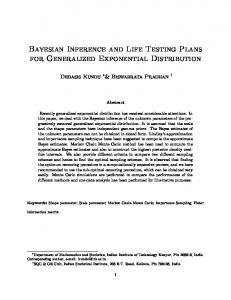
As the joint prior on (λ1 , λ2 ) is little complicated, a gray-scale plot is provided in Figure 1 for different values of hyper-parameters. In the plot black color represents the maximum value of density function, whereas white color represents the minimum value (which is zero) of density function. We have taken b = 1.0 only, as different values of b only effects the spread of the density function keeping the shape fixed.
8
4
1.80
3
1.35
15
0.0600 0.0450
2
0.90
1
0.45
0
0.00
λ2
λ2
10 0.0300 5
0
1
2
3
0.0150 0
4
0.0000 0
5
10
15
λ1
λ1 (a) a = 2.0, b = 1.0, c = 3.5, d = 2.5
4
1.80
3
1.35
(b) a = 7.0, b = 1.0, c = 3.5, d = 2.5
15
0.0600 0.0450
2
0.90
1
0.45
0
0
λ2
λ2
10 0.0300 5
0
1
2
3
0.0150 0
4
0.0000 0
5
λ1
10
15
λ1
(c) a = 2.0, b = 1.0, c = 2.5, d = 3.5
4
1.00
3
0.75
(d) a = 7.0, b = 1.0, c = 2.5, d = 3.5
15
0.0300 0.0225
2
0.50
1
0.25
0
0.00
λ2
λ2
10 0.0150 5
0
1
2
3
0.0075 0
4
0.0000 0
λ1
5
10
15
λ1
(e) a = 2.0, b = 1.0, c = 1.0, d = 1.0
(f) a = 7.0, b = 1.0, c = 1.0, d = 1.0
Figure 1: Plot of prior density for different values of hyper-parameters.
9
4
Maximum Likelihood Estimator under Type-I Censoring Scheme
In this section we present maximum likelihood estimation of the scale parameters under the restriction λ1 ≤ λ2 , when data are Type-I censored. Let n∗1 and n∗2 denote the number of failures before the time τ1 and between τ1 and τ2 , respectively. They can be zero also. Let τ ∗ and n∗ denote the termination time of the experiment and total number of failures observed before τ ∗ , respectively. Note that τ ∗ and n∗ depend on the censoring scheme. In case of Type-I censoring scheme, τ ∗ = τ2 . For Case (a): n∗1 = 0, n∗2 = n2 > 0, Case (b): n∗1 = n1 > 0, n∗2 = n2 > 0, Case (c): n∗1 = n1 > 0, n∗2 = 0. In all the cases n∗ = n∗1 + n∗2 . Based on the observations from a simple SSLT under Type-I censoring scheme, the likelihood can be written as n∗
n∗
l1 (λ1 , λ2 | Data) ∝ λ1 1 λ2 2 e−λ1 d1 −λ2 d2 , where d1 =
∑n∗1
j=1 tj:n
+ (n − n∗1 )τ1 , d2 =
∑n∗
j=n∗1 +1 (tj:n
(8)
− τ1 ) + (n − n∗ )(τ ∗ − τ1 ). Note that d1
and d2 are the total time elapsed by all the units at stress level s1 and s2 , respectively. The unrestricted MLEs of λ1 and λ2 are given by ∗ b∗ = n1 λ 1 d1
and
∗ b ∗ = n2 . λ 2 d2
b∗ ≤ λ b∗ , MLEs of the scale parameters under the restriction λ1 ≤ λ2 are given by Clearly, if λ 1 2 n∗1 ∗ b b λ1 = λ1 = d1
and
n∗2 ∗ b b λ1 = λ1 = . d2
b∗ , maximization of l1 (λ1 , λ2 | Data) under b∗ > λ As l1 (λ1 , λ2 | Data) is unimodal function, if λ 2 1 the order restriction λ1 ≤ λ2 is equivalent to maximization of l1 (λ1 , λ2 | Data) under λ1 = λ2 , and hence, in this case the MLEs of the scale parameters under the restriction λ1 ≤ λ2 are given by ∗ ∗ b1 = λ b 2 = n1 + n2 . λ d1 + d2
10
5
Posterior Analysis under Different Censoring Schemes
5.1
Type-I Censoring Scheme
Based on the likelihood function in (8), priors π1 (·) and π2 (·) mentioned in Section 3, posterior density function of (α, λ2 ) becomes ∗
l2 (α, λ2 | Data) ∝ αn1 +c−1 (1 − α)d−1 λn2
∗ +a−1
e−λ2 (d1 α+d2 +b)
if 0 < α < 1, λ2 > 0.
(9)
The right hand side of (9) is integrable if n∗1 + c > 0 and n∗ + a > 0. Bayes estimate of some function of α and λ2 , say g(α, λ2 ), with respect to the squared error loss function, is posterior expectation of g(α, λ2 ), i.e., ∫ 1∫ ∞ gb(α, λ2 ) = g(α, λ2 )l2 (α, λ2 | Data)dλ2 dα. 0
(10)
0
Unfortunately, the close form of (10) cannot be obtained in most of the cases. One may use numerical techniques to compute (10). Alternatively, other approximations, like Lindey’s approximation, can be used to compute (10). However, CRI for a parametric function cannot be constructed by these numerical methods. Hence we propose to use importance sampling to compute BE as well as to construct CRI of a parametric function in this article. Note that for 0 < α < 1 and λ2 > 0, l2 (α, λ2 | Data) can be expressed as l2 (α, λ2 | Data) = l3 (α | Data) × l4 (λ2 | α, Data),
(11)
where ∗
αn1 +c−1 (1 − α)d−1 , l3 (α | Data) = c1 (d1 α + d2 + b)a+n∗
(12)
and ∗
{d1 α + d2 + b}a+n a+n∗ −1 −λ2 (d1 α+d2 +b) e . l4 (λ2 | α, Data) = λ2 Γ(a + n∗ )
(13)
The proportionality constant, c1 , for the posterior distribution of α given in (12) can be found using numerical techniques. However, generation from (12) is not a trivial issue. Hence, we propose to use the importance sampling (see Algorithm 5.1) to compute the BE and as well as to construct CRI of g(α, λ2 ) noting the following representation of l2 (α, λ2 | Data). For 11
0 < α < 1 and λ2 > 0 l2 (α, λ2 | Data) = c1 w1 (α) × l4 (λ2 | α, Data),
(14)
where ∗
w1 (α) =
αn1 +c−1 (1 − α)d−1 . (d1 α + d2 + b)a+n∗
(15)
Algorithm 5.1 Step 1. Generate α1 from U(0, 1) distribution. Step 2. For the given α1 , generate λ21 from (13). Step 3. Continue the process M times to get {(α1 , λ21 ), . . ., (αM , λ2M )}. Step 4. Compute gi = g(αi , λ2i ); i = 1, 2, . . . , M . c1 w1 (αi ) ; i = 1, 2, . . . , M . M Step 6. Compute the BE of g(α, λ2 ) as Step 5. Calculate the weights w1i =
gb(α, λ2 ) =
M ∑
w1j gj .
j=1
Step 7. To construct a 100(1 − γ)%, 0 < γ < 1, CRI of g(α, λ2 ), first order gj for j = 1, . . . , M , say g(1) < g(2) < . . . < g(M ) , and order w1j accordingly to get w1(1) , w1(2) , . . ., w1(M ) . Note that w1(1) , w1(2) , . . ., w1(M ) may not be ordered. A 100(1 − γ)% CRI can be obtained as (g(j1 ) , g(j2 ) ), where j1 and j2 satisfy j1 , j2 ∈ {1, 2, . . . , M },
j 1 < j2 ,
j2 ∑ i=j1
∑
j2 +1
w1(i) ≤ 1 − γ