Apr 12, 2016 - We call it the ORIentation-boosted vOxel Net â ORION. We experimented with three different variants to implement this concept. In all three ...
arXiv:1604.03351v1 [cs.CV] 12 Apr 2016
1
Orientation-boosted Voxel Nets for 3D Object Recognition Nima Sedaghat
Mohammadreza Zolfaghari
Thomas Brox
Computer Vision Group, University of Freiburg, Germany
Abstract. Recent work has shown good recognition results in 3D data using 3D convolutional networks. In this paper, we argue that the object orientation plays an important role in 3D recognition. To this end, we approach the category-level classification task as a multi-task problem, in which the network is forced to predict the pose of the object in addition to the class label. We show that this yields significant improvements in the classification results. We implemented different network architectures for this purpose and tested them on different datasets representing various 3D data sources: LiDAR data, CAD models and RGBD images. We report state-of-the-art results on classification, and analyze the effects of orientation-boosting on the dominant signal paths in the network. Keywords: 3D ConvNet, CNN, Orientation, Voxel Grid, Multi-task Learning, Recognition, Point-cloud
Introduction
Various devices producing 3D point clouds have become widely applicable in recent years, e.g., range sensors in cars and robots or depth cameras like the Kinect. Structure from motion and SLAM approaches have become quite mature and generate reasonable point clouds, too. While 2D recognition is largely dominated by deep learning for a few years, counterparts for 3D recognition have appeared only recently [1,2]. Since the features for recognition are no longer designed manually but learned by the network, deep learning is very generic regarding the input data. Changing from 2D to 3D recognition requires only relatively small conceptual changes in the network architecture. In this work, we will elaborate on 3D recognition using 3D convolutional networks, where we focus on the aspect of auxiliary task learning. Usually, a deep network is directly trained on the task of interest, i.e., if we care about the class labels of a point cloud, the network is trained to produce correct class labels. There is nothing wrong with this strategy, except that the network must manage to learn the most important concepts to be successful on this task. Since the underlying optimization problem is very complex, training often fails to learn some important concepts.
2
Sedaghat, Zolfaghari and Brox
Chair?
Chair
Fig. 1: Symbolic illustration of how training on orientations helps with better category-level classification in a neural net. The one on the top is a network just trained for classification, while the one on the bottom, can resemble the Cascade architecture of section 3.3.
In the present paper, we focus on the concept of object orientation. The actual task only cares about the object label, not its orientation. However, to produce the correct class label, at least some part of the network representation must be invariant to the orientation of the object, which is not trivial in 3D. Effectively, to be successful on the classification task, the network must also solve the orientation estimation task, but the loss function does not give any direct indication that solving this auxiliary task is important. We show that forcing the network to produce the correct orientation during training, increases its classification accuracy significantly. We evaluated three slightly different network architectures that implement this idea. We used 4 different datasets representing the large variety of acquisition methods for point clouds: laser range scanners, RGB-D images and CAD models. The input to the network is an object candidate obtained from any of these data sources, which is fed to the network as an occupancy grid. We compare the baseline without orientation information to the orientation-boosted versions and obtain improved results in all experiments. We also compare to the the ex-
Orientation-boosted Voxel Nets for 3D Object Recognition
3
Fig. 2: Basic Orientation Boosting. Class labels and orientation labels are two separate outputs. The number of orientation labels assigned to each class can be different to the others. Both outputs contribute to the training equally – with the same weight.
isting methods and achieve state-of-the-art results using our orientation-boosted networks in most of the experiments.
2
Related Work
Most works on 3D object recognition rely on handcrafted feature descriptors, such as Point Feature Histograms [3,4], 3D Shape Context [5], or Spin Images [6]. Descriptors based on surface normals have been around too, and very popular since as early as 1984 [7,8]. [9] gives an extensive survey on such descriptors. Feature learning for 3D recognition has first appeared in the context of RGBD images, where depth is treated as an additional input channel [10,11,12]. Thus, the approaches are conceptually very similar to feature learning in images. [13] fits and projects 3D synthetic models into the image plane. 3D convolutional neural networks (CNNs) have found their way into this research field with works on videos. Tran et al. [14] use video frame stacks as a 3D signal to approach multiple video classification tasks using their 3D CNN, called C3D. Of course, 3D CNNs are not limited to videos, but can be applied also to other three-dimensional inputs, such as point clouds, as in our work. The most closely related works are by Wu et al. [1] and Maturana & Sherer [2], namely 3D ShapeNets and VoxNet, to which we compare our results. Wu et al. use a Deep Belief Network to represent geometric 3D shapes as a probability distribution of binary variables on a 3D voxel grid. They use their method for shape completion from depth maps, too. The ModelNet dataset was introduced along with their work. The VoxNet [2] is composed of a simple but effective CNN, accepting as input voxel grids similar to Wu et al. [1]. Their work shows state-of-the-art results in many experiments. In both of these works the training data is augmented by rotating the object to make the network learn a feature representation that is invariant to rotation. However, in contrast to the networks
4
Sedaghat, Zolfaghari and Brox
proposed in this paper, the network is not enforced to output the object orientation, but only its class label. While in principle, the loss on the class label alone should be sufficient motivation for the network to learn an invariant representation, our experiments show that an explicit loss on the orientation helps the network to learn such representation. In [15] the authors do take advantage of the object pose, explicitly, by rendering the 3D objects from multiple viewpoints and using the projected images in a combined architecture of 2D CNNs to extract features. However, this method still relies on the appearance of the objects in images, which only works well for dense surfaces that can be rendered. For sparse and potentially incomplete point clouds, the approach is not applicable. The authors of [16] focus on 3D object detection in RGB-D scenes. In their work they utilize a 3D CNN for 3D object bounding box suggestion. For the recognition part, they combine geometric features in 3D and color features in 2D. Several 3D datasets have become available recently. There are many datasets with point-clouds obtained from range-scanners, such as the Sydney Urban Objects used in [17]. The Sydney dataset is of special interest in our work as it lets us compare our results to the work of [2]. SUN-RGBD [18] and SUN-3D [19] gather some Reconstructed point-clouds and RGB-D datasets in one place and in some cases they also add extra annotations to the original datasets. We use the annotations provided for NYU-Depth V2 dataset [20] by SUN-RGBD in this work. ModelNet is a dataset consisting of synthetic 3D object models [2]. Sedaghat & Brox [21] created a dataset of annotated 3D point-clouds of cars from monocular videos using structure from motion and some assumptions about the scene structure.
3
Method / Implementation
The core network architecture is based on VoxNet [2] and illustrated in Fig. 2. It takes a 3D voxel grid as input and contains two convolutional layers with 3D filters and two fully connected layers. Although this choice may not be optimal, we kept it to be able to directly compare our modification with VoxNet. Point clouds or CAD models are converted to voxel grids (occupancy grids). For the NYUv2 dataset we used the provided tools for the conversion and for the other datasets we implemented our own version. We tried both binary-valued and continuous-valued grids. In the end, the difference in the results was negligible and thus we report the results of the former one. We modify this architecture by adding orientation estimation as another task. We call it the ORIentation-boosted vOxel Net – ORION. We experimented with three different variants to implement this concept. In all three cases, we consider orientation estimation as a classification problem by quantizing the orientations. Without loss of generality, we only consider rotation around the zaxis as the most frequent case in practical applications. Actually the orientation is a continuous parameter and the network could also be trained to provide such an output. However, this would make it more difficult to combine the loss of
Orientation-boosted Voxel Nets for 3D Object Recognition
5
(a) Basic Architecture
(b) Fusion Architecture
(c) Fine-to-Coarse Architecture
Fig. 3: Suggested architectures for combination of orientation and class labels. On top the “Basic” architecture is depicted where the outputs are simply combined in a parallel form. In the second architecture, namely “Fusion”, we enforce reestimation of a final class label, based on the activations of the output layers of “Basic”. Here, LCf is the loss computed on the last layer. The architecture on the bottom is the smarter “Fine-to-Coarse” cascade combination, where the class output is directly obtained from the orientation output activations.
6
Sedaghat, Zolfaghari and Brox
the object classification task LC with the loss of the orientation estimation LO . Choosing a cross-entropy loss for both tasks, we can just sum them up L = (1 − w)LC + wLO
(1)
and use equal weights, i.e., w = 0.5. We found in our experiments that the results do not depend on the exact choice of the weight w around this value. The network has output nodes for the product label space of classes and orientations. This is because we are not actually interested in the orientation output, but in improving the classification accuracy. Sharing the orientation output for all classes would make the network learn features shared among classes to determine the orientation, which is the opposite of what we want. The number of orientation labels per object class differs. This is detailed in Table 1 for the Sydney dataset as an example. The idea is that we do not want the network to try to differentiate between, e.g., a table and it’s 180◦ rotated counterpart. For the same reason, to rotationally symmetric objects, such as poles, or rotationally neutral ones, such as trees to which no meaningful azimuth label can be assigned, we dedicate only a single node. In the following, we elaborate on the three suggested architectures. In all of them we tried to restrict the modifications just to the additional orientation estimation in order to precisely analyze just the effect of orientation-boosting. 3.1
Basic Orientation-Boosting
The most basic architecture that integrates the auxiliary task of orientation estimation is depicted in Figures 2 & 3(a). The core architecture is the same as VoxNet [2]. However, we call this slightly modified network “ORION Basic”, as we simply extend the class output by additional orientation output units. The orientation output is formed via the ’fc4o’ layer. We compute two softmax loss values for class and orientation outputs, LC & LO respectively, and use them with equal weights to update the network parameters during training. We argue that this simple modification affects the inner layers such that the learned features are more suitable for both outputs. 3.2
Fusion of Orientation and Classification
The architecture introduced in the previous section tries to boost the estimated class labels just by forcing the network to predict the orientation. However, it does not benefit from the estimated labels and relies only on their effects on the inner layers. In the second architecture, we allow the network to benefit from these results via a ’fusion’ block, as shown in Figure 3(b). This fusion block concatenates the primary class and orientation nodes, and connects them to a secondary class output using a fully connected layer. The idea is to enforce some degree of consistency between the primary class and orientation outputs: the “building class” node should not fire simultaneously with the “car-40◦ ” node.
Orientation-boosted Voxel Nets for 3D Object Recognition
7
To this end, we compute a loss for the final class output, while still having the two primary losses: L = wC LC + wO LO + wCf LCf
(2)
where LC , LO & LCf are the losses computed on the primary class output, the orientation output, and the secondary class output, respectively. We use the same weight of 1/3 for all three components. 3.3
Fine-to-Coarse (Cascade) Combination
We tested another architecture that combines the two tasks in a smarter way – Figure 3(c). The idea is to obtain the class labels directly from the orientation activations, which can be seen as a finer representation of the class labels. Although the weights connecting the orientation nodes to the class nodes follow a simple and predictable pattern, this does not mean that the class nodes are unnecessary here; the class loss is still there and plays an important role in enforcing the consistency between the two outputs – by contributing in the multi-task objective. As in ORION Basic, we set wC = wO = 0.5.
4
Experiments & Datasets
We train and test our networks on four datasets, three of which are illustrated in Figure 4. As mentioned before, we have chosen the datasets such that they represent different data sources – except the first two, which differ in size and object classes. In all of the experiments, we again take advantage of the orientation concept, by feeding into the network multiple orientations of the test object and making the final decision based on all the results. This so-called voting is done by summing up the activations of the output layer throughout all the rotations and then picking the argmax as the class label. 4.1
Sydney Urban Objects - LiDAR/Pointcloud
This dataset consists of LiDAR scans of 631 objects in 26 categories. The point clouds representing the objects in this dataset are always incomplete, as they are only seen by the LiDAR sensor from a single viewpoint. In this sense they are similar to point clouds obtained from RGB-D images. Therefore the quality of the objects are by no means comparable to synthetic 3D objects, making classification a challenging task, even for human eyes; see Figure 4. This dataset is also of special interest in our category-level classification, as it provides a tough categorization of vehicles: 4wd, bus, car, truck, ute and van are all distinct categories. We use the same settings as [2] to make our results comparable to theirs. The point clouds are converted to voxel-grids of size 32x32x32, in which the object occupies a 28x28x28 space. Zero-paddings of size 2 is used on each side to enable displacement augmentation during training. We also annotated
8
Sedaghat, Zolfaghari and Brox
Fig. 4: Examples from three datasets. On top- and middle-left, two exemplar scenes from the NYUv2 [20] & Sydney [17] datasets are depicted respectively. On their opposite sides sample objects from the scenes are shown. Each row shows the same object in multiple rotations. On the bottom samples from the Modelnet dataset are displayed. Objects of the well-known KITTI dataset are similar to the ones in Sydney, and are not showed here due to space limitations.
the orientations to make the data suitable for our method. These we will provide to the public. The number of orientation classes assigned to each object class is presented in Table 1. 4.2
KITTI - LiDAR/Pointcloud
The KTTI dataset [22] contains 7481 training images and 7518 test images in its object detection task. Each image represents a scene which also comes with a corresponding Velodyne point cloud. 2D and 3D bounding box annotations are provided in the images. Using the provided camera calibration parameters they can be converted into the coordinates of the Velodyne scanner. The annotations are publicly available only for the training set. Thus, we split the original training set to 80% and 20% subsets for training and testing, respectively. This dataset
Orientation-boosted Voxel Nets for 3D Object Recognition
9
4wd building bus car pedestrian pillar pole lights #Orientation Nodes
18
9
9
18
1
1
1
9
Table 1: Number of orientation output nodes assigned to each class in the Sydney dataset. We show only a subset of classes due to space limitations. has fewer object classes compared to the Sydney dataset, and the ’Car’, ’Pedestrian’ and ’Cyclist’ classes are the dominant ones used in many experiments. We tested our method with all classes. The dataset comprises a large number of objects at different difficulty levels, which eliminates the need for augmentation in our experiments. We used grids of size 28x28x28 on this dataset. We consider a maximum of 18 discretization levels for the object orientations. 4.3
NYUv2 - Kinect/RGBD
This dataset consists of an overall number of 2808 RGBD images, corresponding to 10 object classes. The class types are shared with the ModelNet10 dataset. We used voxel grids of size 32x32x32, which contain the main object in the size of 28x28x28. The rest includes the context of the object and each object has a maximum number of 12 rotations. The dataset does not provide orientation annotations and therefore we used the annotations provided by the SUN-RGBD benchmark with manual correction of some annotations. 4.4
ModelNet - Synthetic/CAD
This dataset is composed of synthetic CAD models. We use the so called ModelNet10 subset, which consists of uniformly aligned objects of the same classes as in the NYUv2 dataset. The object meshes were converted to voxel grids of size 28x28x28, similar to the NYUv2 settings.
5
Results
The classification results on all datasets are shown in Table 2. For the Sydney Urban Objects dataset, we report the average F1 score, weighted by class support, as used by [1], to be able to compare our results to their work. This weighted average takes into account that the classes in this dataset are unbalanced. For the other datasets we report the average accuracy. The Sydney dataset provides 4 folds/subsets to be used for cross-validation; in each experiment three folds are for training and one for testing. We also follow this standard in our experiments on this dataset. To show the significance of the orientation sensitive networks over the raw classification baseline, we show in Table 3 that the orientation sensitive networks outperform the baseline on all folds, with only one exception for the ORION Basic network. Moreover, we train and test with at least two versions of the same
10
Sedaghat, Zolfaghari and Brox Dataset Sydney Method↓ Recursive D [23] Recursive D+C [23] Triangle+SVM [17] GFH+SVM [24] ShapeNet [1] DeepPano [25] VoxNet [2] Our Baseline ORION Basic ORION Fusion ORION F2C
F1
mean
67.1 71.0 72. 74.8 76.7 77.8 77.3
ModelNet10
NYU
KITTI
std. mean
std.
mean std. mean std.
0.0 0.1 0.1 0.4
0.3 0.1 0.1 0.0
37.6 44.8 57.9 71. 75.5 76.3 75.9 75.7
83.5 85.5 92 92.8 93.4 93.5 93.8
0.1 0.3 0.6 0.2
93.0 93.5 93.7 93.6
0.1 0.1 0.1 0.2
Table 2: Classification Results. Here we report the overall accuracy of various methods on different datasets, except for the Sydney dataset where we report the weighted average over F1 score. Introduction of orientation has clearly made improvements in all cases – all shown in percentages. We report the mean and standard deviation (std.) over the same networks trained with different random seed.
network. These versions share the same architectures and training parameters, and differ only in the random seed used during training. We observe that the random seed leads to some fluctuation in the performance, which we can measure by the standard deviation, but not seriously so. The standard deviation indicates the significance of the improvement over the baseline, as well as the fact that the best three results on each dataset belong to the three architectures with additional orientation output.
6
Analysis
To analyze the behavior of the orientation-boosted network, we compare it to its corresponding baseline network. We would like to know the differences between corresponding filters in the two networks. To find this correspondence, we first train the baseline network long enough, so that it reaches a stable state. Then we use the trained net to initialize the weights of the ORION Basic, and continue training with low learning rate. This way we can monitor how the features change in the transition from the baseline, to the orientation-boosted one. In Figure 6 transition of a single filter is depicted, and its response to different rotations of an input object is analyzed. It turns out that the filter tends to become more sensitive to the orientation-specific features of the input object.
Orientation-boosted Voxel Nets for 3D Object Recognition Method↓
11
Foldset 1 Foldset 2 Foldset 3 Foldset 4
Our Baseline ORION Basic ORION Fusion ORION F2C
79.8 83.7 83.7 84.1
75.5 77.3 78.3 76.5
75.6 78.4 80.4 80.5
68.3 67.4 68.7 69
Table 3: Fold by fold measurements on the Sydney dataset. On each fold, the orientation sensitive networks improve over the baseline, with only one exception, indicating the significance of the improvement.
Ground Truth ORION Basic Baseline
4wd 4wd car
Ground Truth table ORION Basic table Baseline nite-stnd
building building bus
bus bus car
desk desk sofa
monitor monitor chair
chair chair table
ute truck ute
toilet chair toilet
bathtub bed table
Fig. 5: Some exemplar classification results. Here we mainly show the examples on which the two networks have performed differently.
Additionally some parts of the object, such as the table legs, show stronger response to the filter in the orientation-boosted network. With such an observation, we tried to analyze the overall behavior of the network for specific object classes, respecting their different orientations. To this end we introduce the “dominant signal-flow path” of the network. The idea is that, although all the nodes and connections of the network contribute to the formation of the output, in some cases there may exist a set of nodes, which have a higher effect in this process for an specific type of object/orientation. To test this, we take this step-by-step approach: First in a forward pass, the class (c) of the object is found. Then we seek to find the highest contributing node of the last hidden layer:
n−1 n−1 ln−1 = arg max{wk,c ak } k
(3)
70 73 74 82 83 82 82
50 22 39 37 35 40 35
62 34 47 71 73 72 74
50 59 59 59 66 63
73 48 60 74 73 73 72
25 41 44 64 62 63 61
t
99 99 99 99
ile
50 47 47 73 71 68 67
84 83 84 87
e
30 10 17 23 26 25 26
m
92 81 69 90 92 91 91
30 19 48 51 50 50
to
96 98 98 97
bl
dr e
83 88 87 87
40 52 52 61 62 60
ta bl e to ile t
31 25 32 40 46 48
ta
68 73 82 84 81 83
tr uc k tr un k ut e va n
tr ee
62 74 66 66 68 68
er on ito r ni gh -s ta nd so fa
sk
99 99 99 99
dr e
86 0 0 76 76 76 76
88 85 86 86
de sk
100 99 100 99 100 100 100 99
ch ai r
ShapeNet [1] Recursive D [23] Recursive D+C [23] Our Baseline ORION Basic ORION Fusion ORION F2C
85 88 88 88
de
ch ai r
be
d
th tu ba
84 92 90 92
ba th tu b be d
Our Baseline ORION Basic ORION Fusion ORION F2C
57 63 75 69 73 72
ss er m on ito r ni gh -s ta nd so fa
37 81 96 57 64 55 82 94 68 73 59 85 97 68 57 63 85 98 73 68 64 86 98 75 72 64 85 97 75 73
ss
59 81 63 79 76 78 b
24 0 48 42 46 43
pe
4w
Triangle+SVM [17] GFH+SVM [24] Our Baseline ORIO Basic ORION Fusion ORION F2C
de s pi t. lla r po le lig ht s sig n
Sedaghat, Zolfaghari and Brox d bu ild bu ing s ca r
12
40 20 50 89 93 91 91
Table 4: Per-class measurements for the Sydney, Modelnet10 and NYUv2 datasets, from top to bottom. We report the F1 Score for the first dataset, and accuracies for the others – shown in percentages.
n−1 where an−1 are the activations of layer n − 1, and wk,c is the weight conk n−1 th necting ak to the c node of layer n. This way we naively assume there is a significant maximum in the contributions and assign its index to ln−1 – which proves to be true in many of our observations. We continue “back-tracing” the signal, to the previous layers. Extension of (3) to the convolutional layers is straight-forward, as we are just interested in finding the index of the node/filter in each layer. In the end, letting ln = c, gives us the vector l with length equal to the number of network layers, keeping the best contributors’ indices in it. Now to depict the “dominant signal-flow path” for a group of objects, we simply obtain l for every member of the group, and plot the histogram of the li s as a column. Figure 12(a) shows such an illustration for a specific class-rotation
Orientation-boosted Voxel Nets for 3D Object Recognition
13
of the objects. It is clearly visible that for many objects of that group, specific nodes have been dominant. In Figure 12(b), the dominant paths of the baseline and ORION Basic networks for some sample object categories of the Modelnet10 dataset are illustrated. It can be seen that in the baseline network, the dominant paths among various rotations of a class share some of their nodes. This is mostly visible in the convolutional layers. On the contrary, the dominant paths in the ORION network rarely follow this rule and have more distributed path nodes. We interpret this as one of the results of orientation-boosting, and a helping factor in better classification abilities of the network.
7
Conclusion
We showed for the task of 3D object classification that learning of certain concepts, such as invariance to object orientation, can be supported by adding the concept as an auxiliary task during training. By forcing the network to produce also the object orientation during training, it achieved better classification results. This finding was consistent on all datasets and enabled us to establish state-of-the-art results on most of them.
14
Sedaghat, Zolfaghari and Brox
iterations ORION ←−−−−−−−−−−−−−−−−−−−−−−−−−−−−−−−−−−−−−−−−−−−−−−−−−−−−−−−−−baseline
←− Object Orientations −→
− higher values −→
Fig. 6: The picture illustrates the activations of one of the nodes of the first layer, while the network transitions from a baseline network to the ORION Basic (top to bottom). The input is always the same object, which has been fed to the network in its possible discretized rotations (columns) at each step (row). We simulated this transition by first training the baseline network and then finetuning our Basic architecture on top of the learned weights. To be able to depict the 3D feature maps, we had to cut out values below a specific threshold. It can be seen that the encoded filter detects more orientation-specific aspects of the object, as it moves forward in learning the orientations. In addition, it seems that the filter is becoming more sensitive to a table rather than only a horizontal surface – notice the table legs appearing in the below rows.
15
fc4
fc3
conv2
conv1
Orientation-boosted Voxel Nets for 3D Object Recognition
ORION baseline
ORION baseline
ORION baseline
ORION baseline
ORION baseline
(a)
←− Object Orientations −→ (b)
Fig. 7: (a) shows the “dominant signal-flow path” of the network, for an exemplar object category-orientation. Each column contains the activations of one layer’s nodes. Obviously the columns are of different sizes. Higher intensities show dominant nodes for the specific group of objects. Details of the steps taken to form such an illustration are explained in the text. In (b), rows represent object classes, while in different columns we show rotations of the objects. So each cell is a specific rotation of a specific object category. It can be seen that in the baseline network, many of the rotations of a class, share nodes in their dominant path, whereas, in the ORION network the paths are more distributed over all the nodes.
16
Sedaghat, Zolfaghari and Brox
References 1. Wu, Z., Song, S., Khosla, A., Yu, F., Zhang, L., Tang, X., Xiao, J.: 3D ShapeNets: A Deep Representation for Volumetric Shapes. In: Proceedings of the IEEE Conference on Computer Vision and Pattern Recognition. (2015) 1912–1920 2. Maturana, D., Scherer, S.: VoxNet: A 3D Convolutional Neural Network for Real-Time Object Recognition. In: Intelligent Robots and Systems (IROS), 2015 IEEE/RSJ International Conference on, IEEE (2015) 922–928 3. Rusu, R.B., Marton, Z.C., Blodow, N., Beetz, M.: Learning informative point classes for the acquisition of object model maps. In: Control, Automation, Robotics and Vision, 2008. ICARCV 2008. 10th International Conference on, IEEE (2008) 643–650 4. Rusu, R.B., Blodow, N., Beetz, M.: Fast point feature histograms (FPFH) for 3D registration. In: Robotics and Automation, 2009. ICRA’09. IEEE International Conference on, IEEE (2009) 3212–3217 00311. 5. K¨ ortgen, M., Park, G.J., Novotni, M., Klein, R.: 3D shape matching with 3D shape contexts. In: The 7th central European seminar on computer graphics. Volume 3. (2003) 5–17 6. Johnson, A.E., Hebert, M.: Using spin images for efficient object recognition in cluttered 3D scenes. Pattern Analysis and Machine Intelligence, IEEE Transactions on 21(5) (1999) 433–449 7. Horn, B.K.P.: Extended gaussian images. Proceedings of the IEEE 72(12) (1984) 1671–1686 8. Patterson IV, A., Mordohai, P., Daniilidis, K.: Object detection from large-scale 3d datasets using bottom-up and top-down descriptors. In: Computer Vision–ECCV 2008. Springer (2008) 553–566 00021. 9. Yulan Guo, Bennamoun, M., Sohel, F., Min Lu, Jianwei Wan: 3D Object Recognition in Cluttered Scenes with Local Surface Features: A Survey. IEEE Transactions on Pattern Analysis and Machine Intelligence 36(11) (November 2014) 2270–2287 10. Farabet, C., Couprie, C., Najman, L., LeCun, Y.: Learning hierarchical features for scene labeling. Pattern Analysis and Machine Intelligence, IEEE Transactions on 35(8) (2013) 1915–1929 11. Couprie, C., Farabet, C., Najman, L., LeCun, Y.: Indoor semantic segmentation using depth information. arXiv preprint arXiv:1301.3572 (2013) 12. Bo, L., Ren, X., Fox, D.: Unsupervised feature learning for RGB-D based object recognition. In: Experimental Robotics, Springer (2013) 387–402 13. Gupta, S., Arbel´ aez, P., Girshick, R., Malik, J.: Aligning 3D Models to RGB-D Images of Cluttered Scenes. In: Proceedings of the IEEE Conference on Computer Vision and Pattern Recognition. (2015) 4731–4740 14. Tran, D., Bourdev, L., Fergus, R., Torresani, L., Paluri, M.: C3D: Generic Features for Video Analysis. arXiv preprint arXiv:1412.0767 (2014) 15. Su, H., Maji, S., Kalogerakis, E., Learned-Miller, E.: Multi-view convolutional neural networks for 3D shape recognition. In: Proceedings of the IEEE International Conference on Computer Vision. (2015) 945–953 16. Song, S., Xiao, J.: Deep Sliding Shapes for Amodal 3D Object Detection in RGB-D Images. arXiv preprint arXiv:1511.02300 (2015) 17. De Deuge, M., Robotics, F., Quadros, A., Hung, C., Douillard, B.: Unsupervised Feature Learning for Classification of Outdoor 3D Scans. (2013) 18. Song, S., Lichtenberg, S.P., Xiao, J.: SUN RGB-D: A RGB-D Scene Understanding Benchmark Suite. In: Proceedings of the IEEE Conference on Computer Vision and Pattern Recognition. (2015) 567–576
Orientation-boosted Voxel Nets for 3D Object Recognition
17
19. Xiao, J., Owens, A., Torralba, A.: SUN3D: A database of big spaces reconstructed using sfm and object labels. In: Computer Vision (ICCV), 2013 IEEE International Conference on, IEEE (2013) 1625–1632 20. Silberman, N., Hoiem, D., Kohli, P., Fergus, R.: Indoor segmentation and support inference from RGBD images. In: Computer Vision–ECCV 2012. Springer (2012) 746–760 21. Sedaghat, N., Brox, T.: Unsupervised Generation of a Viewpoint Annotated Car Dataset from Videos. In: Proceedings of the IEEE International Conference on Computer Vision (ICCV). (2015) 22. Geiger, A., Lenz, P., Urtasun, R.: Are we ready for Autonomous Driving? The KITTI Vision Benchmark Suite. In: Conference on Computer Vision and Pattern Recognition (CVPR). (2012) 23. Socher, R., Huval, B., Bath, B., Manning, C.D., Ng, A.Y.: Convolutional-recursive deep learning for 3d object classification. In: Advances in Neural Information Processing Systems. (2012) 665–673 24. Chen, T., Dai, B., Liu, D., Song, J.: Performance of global descriptors for velodynebased urban object recognition. In: Intelligent Vehicles Symposium Proceedings, 2014 IEEE, IEEE (2014) 667–673 25. Shi, B., Bai, S., Zhou, Z., Bai, X.: DeepPano: Deep Panoramic Representation for 3-D Shape Recognition. IEEE Signal Processing Letters 22(12) (December 2015) 2339–2343
18
Sedaghat, Zolfaghari and Brox
Supplementary Material
Ground Truth ORION Basic Baseline
4wd 4wd car
4wd 4wd car
building building bus
Ground Truth ORION Basic Baseline
car car 4wd
traf.lights traf.lights trunk
traf.sign traf.sign traf.lights
Ground Truth ORION Basic Baseline
4wd van car
pole trunk trunk
trunk pedestrian pedestrian
bus bus car
car car van
trunk trunk trunk trunk pedestrian traf.sign
car car 4wd
trunk trunk pole
ute truck ute
Fig. 8: More results from the classification experiment on the Sydney dataset.
Orientation-boosted Voxel Nets for 3D Object Recognition
Ground Truth ORION Basic Baseline
desk desk table
desk desk table
desk desk sofa
monitor monitor chair
nite-stnd nite-stnd dresser
Ground Truth ORION Basic Baseline
nite-stnd nite-stnd dresser
nite-stnd nite-stnd dresser
nite-stnd nite-stnd dresser
nite-stnd nite-stnd table
table table desk
Ground Truth ORION Basic Baseline
toilet chair toilet
bathtub sofa bathtub
desk nite-stnd nite-stnd
bathtub bed table
desk table table
19
nite-stnd nite-stnd dresser
Fig. 9: More results from the classification experiment on the Modelnet dataset.
20
Sedaghat, Zolfaghari and Brox
Ground Truth ORION Basic Baseline
table table nite-stnd
chair chair table
Ground Truth ORION Basic Baseline
monitor monitor chair
nite-stnd nite-stnd dresser
Ground Truth ORION Basic Baseline
dresser dresser sofa
sofa bed bed
Fig. 10: More results from the classification experiment on the NYUv2 dataset. Objects in this dataset suffer from a high degree of (self-)occlusion. This is specially worse in this figure where we focus only on difficult examples on which at least one network has failed. Each object is displayed from multiple views.
21
ORION baseline
ORION baseline
ORION baseline
ORION baseline
ORION baseline
ORION baseline
ORION baseline
ORION baseline
ORION baseline
Orientation-boosted Voxel Nets for 3D Object Recognition
←− Object Orientations −→
Fig. 11: Dominant signal-flow path comparison for networks trained on the NYUv2 dataset, with and without orientation-boosting. Each row-pair represents one object class. In this figure we compare baseline to the Basic architecture of ORION.
Sedaghat, Zolfaghari and Brox
ORION baseline
ORION baseline
ORION baseline
ORION baseline
ORION baseline
ORION baseline
ORION baseline
ORION baseline
ORION baseline
22
←− Object Orientations −→
Fig. 12: Dominant signal-flow path comparison for networks trained on the Sydney dataset, with and without orientation-boosting. Each row-pair represents one object class. In this figure we compare baseline to the Basic architecture of ORION.