Fig. 1. Kinematic structure of a leg of the PKM Linapod. P, U, S denotes prismatic, universal and spherical joints, respectively. kinematics because it can typically ...
Orientation Workspace Verification for Parallel Kinematic Machines with Constant Leg Length Andreas Pott, Daniel Franitza and Manfred Hiller Chair of Mechatronics University of Duisburg-Essen 47057 Duisburg, Germany Email: {pott, franitza, hiller}@imech.de
Abstract— Compared to serial robots, parallel kinematic machines (PKM) offer superior properties. However, modelling and analysis of PKMs are challenging tasks due to their complicated kinematic structure. In this paper we present methods to analyze the workspace of a class of 6 degree-of-freedom (dof) PKMs with constant leg length. These methods apply interval analysis in order to calculate the orientation workspace and to verify if a certain machine covers a desired workspace. The machines are assembled from a construction kit that defines components like legs, frames, and platforms.
Ui
Ai
bar Si
Bi
ei li
ai
platform Pi
bi
si
I. I NTRODUCTION The calculation of the workspace of parallel kinematic machines (PKM) is a complex task due to the nonlinear kinematics. However, for the design and optimization of PKMs, fast and efficient algorithms are needed to investigate the workspace of a variety of machines. In particular, the orientation workspace that combines both translation and rotation of the platform is important for machine tools. In the past many researchers focused on the calculation of the workspace. In order to calculate the workspace one can mostly distinguish between discretization methods, geometrical methods, and analytical methods. For the discretization method a grid of nodes with position and orientation is defined. Then the kinematics is calculated for each node and it is straightforward to verify whether the kinematics can be solved and to check if joint limits are reached or link interference occurs [1], [2]. The discretization algorithm is simple to implement but is has some serious drawbacks. It is expensive in computational time and the results are limited to the nodes of the grid. Thus, we cannot guarantee that the space between two valid nodes is acceptable, too. Using geometrical methods the constant orientation workspace can be calculated as intersection of simple geometrical objects [3]. The accessible pivot points for e.g. PUS (prismatic joint, universal joint, spherical joint) and UPS legs form a cylinder and a sphere, respectively. Constraints on the joints and on the articulated coordinates can be introduced through further restrictions on the geometrical entities and the intersection of these objects can be done with the techniques that are known form computer aided design (CAD). Analytical methods investigate the properties of the kinematic transmission. Most approaches are based on the inverse
KTCP
ni r TCP ci base
Ci
K0 Fig. 1. Kinematic structure of a leg of the PKM Linapod. P, U , S denotes prismatic, universal and spherical joints, respectively.
kinematics because it can typically be solved in closed form and it is easier to distinguish between multiple solutions. Further on, the inverse kinematics is normally formulated in cartesian coordinates. In this paper we present algorithms to calculate and to verify a given orientation workspace of a parallel kinematic machine tool with constant leg lengths. We consider especially the tilt angles of the mobile platform that are relevant for machine tools in practice. The presented algorithms are mainly based on two issues: symbolic solutions of the inverse kinematics and interval analysis of these equations. In section II, the symbolic solution of inverse kinematics is recalled. The procedure for the workspace calculation and verification with interval analysis is presented in section III. Section IV introduces a modular kinematic model for PKMs. Examples and simulation results are given in section V. Finally, in section VI we draw some conclusions. II. S YMBOLIC S OLUTION OF THE I NVERSE K INEMATICS It is well known that it is possible to determine a symbolic solution of inverse kinematics of PKMs [4]. Therefore, we
U
P S TCP
Fig. 2.
Kinetostatic model of the PKM Linapod
will only briefly sketch how the solution is derived because the workspace verification algorithm is based on this solution. The solution of the inverse kinematics of PKMs with constant leg length differ slightly from the more common Gough-type PKM with UPS legs. A mobile platform is actuated through six linear drives that move six legs of constant length li (i = 1, ..6 for the six legs). The frame K0 denotes the world coordinate system and KTCP is the frame that is attached to the mobile platform. The rotation matrix RTCP describes the relative orientation of KTCP with respect to K0 . The pivot points of the leg are denoted with Ai and Bi , respectively (Fig. 1). The actuators move on the line which is defined by the base point Ci and the direction ni . Using a vector loop, yields the closure condition li2 = (ci + ni si − r TCP − RTCP bi )2
(1)
and we can solve for the unknown si r 1 . si = −ni di ± (ni . di )2 − d2i − li2 , (2) 4 with di = ci − r TCP − RTCP bi . The different signs in (2) correspond to different assembly modes of the PKM. Since we know how the PKM at hand is assembled we can choose typically the same sign for all six legs. For the rotation matrix RTCP we use an approach that is based on the expected motions of the platform for machine tools. It should be possible to tilt the platform with an angle ϕ in an arbitrary direction β. Therefore, we introduce a rotation of ϕ about the axis u = (cos β, sin β, 0)T . The RODRIGUES formula yields s2β cϕ + c2β cβ sβ (1 − cϕ ) sϕ sβ cϕ c2β + s2β −sϕ cβ , (3) R(u, ϕ) = cβ sβ (1 − cϕ ) −sϕ sβ sϕ cβ cϕ
where sβ and cβ denote sin β and cos β, respectively. Note that this parameterization of the orientation of the platform covers those orientations we are interested in for machine tools though the intervals β ∈ [0..2π], ϕ ∈ [0.. π2 ]. For application like control other parameters that correspond to the same orientations may be more suitable. In order to calculate the machine geometry dependent vectors ai , bi , ni , we have to introduce a parameterization that describes the variety of machines we want to study. Thus, the the parameters of the Linapod (Fig. II) are briefly introduced. The base points Ci of the linear drives are distributed on a circle around K0 with radius rB . Since there are two drives mounted on one guideway the tangential offset ∆a tends to be small1 and has alternating directions for the upper and the lower drive. Negative values for ∆a are correlated to crossing bars while the bars are almost parallel for positiv ∆a. In the parameterization of the Linapod the length li of the legs is set to two different length lu and ll < lu for the upper legs and the lower legs, respectively. The pivot points on the platform Bi are arranged on circles in two parallel plains for the two groups of legs. The axis through the center of the circles is the z-axis of frame KTCP which is perpendicular to the plane of the circles. The radii of the circles are ru and rl for the upper and the lower circle, respectively. The distance between the plains is ∆h and the pivot points on the circles are mutually rotated by ∆α. III. W ORKSPACE V ERIFICATION WITH I NTERVAL A NALYSIS Interval analysis [5] is a useful mathematical technique to calculate bounds for functions and to solve systems of equations. It was applied to PKMs for the determination of the dexterous workspace [6], trajectory verification [7], and the determination of the workspace of Gough-type PKMs [8]. For the workspace verification we need to set up a number of constraints that define conditions whether a given interval is part of the workspace or not. The basic set of constraints is provides through the inverse kinematics. We can conclude from (2) that a a real solution for si can be found if the radicand is positive. Additionally, we can check if the solution si is in the range smin < si < smax which are the bounds of the prismatic joints. This consideration yields a system of inequalities Φ > 0 that must be fulfilled inside the workspace. The basic idea of the presented algorithms is to exploit the result from an interval evaluation of the constraint inequalities. We evaluate a constraint f (y 0 ) > 0, y 0 ∈ IIn , with interval analysis and we get an interval [f , f ] as result. If the lower bound of the result fulfills f > 0 we know that the inequality holds for any y ∈ y 0 and we store it in a list as valid interval. On the other hand, if f < 0 then the inequality cannot be fulfilled for any y ∈ y 0 and this interval is denoted as invalid. In any other case we cannot make a statement for the whole interval and the interval is called uncertain. Since 1 large values for ∆a are possible but require the construction of a machine with six instead of three guideways
the interval evaluation of a function may overestimate the bounds, we neither know at this point if there are any valid or invalid value for y ∈ y 0 . Therefore, we split the interval by bisection and repeat the evaluation for the smaller intervals until we get a reliable statement (valid or invalid). When we run this algorithm on a computer we have to interrupt the computation when the considered intervals are smaller than a given threshold ∆h. Based on this concept we propose two algorithms: a workspace verification algorithm and a workspace determination algorithm. For the verification algorithm the desired workspace is given as y 0 and we start to test the given workspace as interval. If the bisection leads to at least one invalid interval which does not fulfill the constraints, the algorithm is terminated and reports that the desired workspace is not valid. On the other hand, if the algorithm can subdivide the desired workspace into a finite number of valid intervals we can guarantee that the whole region y 0 belongs to the workspace. The workspace calculation algorithm starts with an interval y 0 that covers the whole region where we expect the workspace to be. The initial interval can be estimated from the length of the legs li and the size rb of the machine frame. Then the subdivision algorithm is used to determine the valid regions of the workspace where the valid intervals are stored in a list. The algorithm is terminated if the intervals are smaller than a given threshold ε and we can estimate the error through the number of uncertain intervals and their volume. A. Reduction of workspace parameter set for Linapod The computation time of the interval bisection algorithm highly depends on the number of interval variables because they determine how many bisection must be made. In general, we have to take into account one interval variable for each dof of the mechanism. Hence for the machine Linapod six interval variables are needed to parameterize the general motion of the platform and therefore to characterize the workspace. On the other hand we generate 26 new intervals in each stage of the bisection process which results in a very large number of interval evaluations that needs to be done for the algorithm. Therefore, we will exploit some special properties of the Linapod in order to reduce the computational effort. From the arrangement of the prismatic joints it can be concluded that the workspace is invariant with respect to translations in the z-direction of the world coordinate system K0 . Thus, we can separate the investigation of the workspace in z-direction from the other directions since they are naturally decoupled. Now we consider the orientations that are needed for machine tools. Since the tool rotates, it is not necessary to orientate the platform along this axis and we introduce the rotation matrix (3) which does not regard orientation with respect to the tool axis. Therefore, the parameter set is reduced to the four parameter y 0 = (x, y, β, ϕ)T . For the position (x, y) we start with the desired range of the workspace. We set β = [0, 2π] to provide tilt in any direction and for ϕ we
Bi
λi dij ei
eij , λij
Bj
Ai ej
λj
Aj Fig. 3.
Distance between two finite line segments
use the interval [0, ϕmax ] where ϕmax is the maximal desired tilt angle. B. Link Interference Check The interference of links and joints significantly restricts the workspace of many PKMs [9]. Thus, it is important to verify if the kinematical reachable workspace is free of link interference or at least to check whether the required (mostly rectangular) workspace may be used without collisions of the components. The most frequent problem in this field is the calculation of the distance between two finite line segments (Fig. III-B). This problem can be easily solved for given points Ai , Bi , Aj , Bj although we have to distinguish between quite a number of special cases where lines are parallel, have identical points etc. This distinction of cases undermines the application of interval analysis in order to perform the calculation for the whole workspace or at least for a region that is defined by intervals of the input variables. The calculation may be simplified by calculating the distance dij between the infinite lines through Ai , Bi and Aj , Bj with ¯ ¯ ¯ ei × ej ¯ ¯ (4) dij = ¯ (ai − aj )¯¯ |ei × ej | but this implies unacceptable errors e.g. if both line segments lie in a common plain. Therefore, we propose a simple interval formula that is directly related to the original problem. Given line segments gi with gi : xi = ai + λi (bi − ai ),
λi ∈ [0..1], i = 1, 2, ..6
we are searching for the supremum dmin of _ dij = |xi − xj | λi , λj ∈ [0..1], i 6= j.
(5)
(6)
By introducing λi , λj ∈ II as intervals we can replace the distinction of cases by a normal interval evaluation of a simple norm function and we receive dmin < dij = |ai + λi (bi − ai ) − aj − λj (bj − aj )|,
(7)
where 1 ≤ i ≤ 6, 1 ≤ j ≤ 6, i 6= j as additional inequations that take into account the link interference and we can add them to the system Φ > 0.
PKM
B1
platform B5 B6
a) Fig. 4.
b) Different types of legs: a) UPS and b) PUS
L5
L2
L1
KTCP
L6
B2
frame A1
A2
K0
A6 A5
C. Joint limits Joint limits in the passive and active joints can be easily validated once we have a formula to calculate the angles θ of the joints which is a well known problem [10]. Typically, we have inequalities of the form θmin ≤ θ(w) ≤ θmax and we can add these inequations to our system Φ > 0. D. Optimization of the System of Equations As shown above different issues limit the feasible workspace of a PKM. These conditions can be expressed in inequalities Φ > 0 of interval functions. The computational effort of the bisection process mainly depends on the number of interval variables. Thus, we have to avoid the evaluation of subsets of inequations that imply a large number of interval variables. Most of the inequations are pose dependent and therefore we have to perform the bisection for w = (x, y, ϕ, β). On the other hand, the λi occurs always in pairs in the inequations (7). Thus, it is cheeper to perform the bisection for 15 single inequations in 6 interval variables instead of one system of 15 inequations in 10 interval variables since the computational time for the bisection process is roughly proportional to 2n where n is the number of interval variables. IV. T OPOLOGICAL S YNTHESIS AND AUTOMATIC M ODEL A SSEMBLY In order to study a wide range of machine types, a generic approach for the modelling of PKM was investigated. Since PKMs tend to be symmetric and different types of PKM have similar components a modular design was used. In a first step we divide the machine into three types of components: frames, platforms and legs. For the kinematic modelling of PKM we choose the kinetostatic method [10] with the C++ a a library M a aBILE [11]. The machine frame defines for a number nf of pivot points Ai the position and orientation. The mobile platform introduces the position and orientation of np pivot point Bi . Furthermore, the platform defines the type and number of degrees-of-freedom (dof) f at the TCP. Finally, we introduce different types of legs. The most common legs for PKMs are PUS and UPS structures each consisting of prismatic, universal, and spherical joints (Fig. 4). Each of these structures
Fig. 5.
Platform and machine frame modules
provides one dof and one constraint. It is also possible to utilize more complicated leg modules. The λ-leg e.g. has two input pivot points for the machine frame but only one output pivot point for the platform. It has two dof and provides two constraints. A class called generic machine assembly module constructs a kinetostatic model [10] from the components introduced above. First we have to attach the legs to the platform and frame. For the inverse kinematics all steps to calculate the generalized coordinates depend only on the local properties of each leg. Therefore, we can implement methods for each legs to solve the inverse kinematics on its own. For the direct kinematics the legs provide constraints that characterize which motions can be transmitted. The generic machine assembly module collects the constraints form the legs and the generalized coordinates from the platform in order to combine them to a nonlinear system of equations. Then a numerical procedure like a N EWTON-R APHSON-algorithm is applied to solve the direct kinematics. Once the position of the platform is determined we can use local methods from the legs to calculate the complementary variables of the passive joints in each kinematic loop. The resulting kinetostatic model can be used for a wide range of functions for kinematic analysis e.g. direct and inverse kinematics, calculation of the Jacobian [10] and dexterity indexes, error analysis [12], static analysis, stiffness matrix, and equations of motion [13]. V. S IMULATION R ESULTS We demonstrate the workspace calculation and verification method with the 6 dof parallel kinematic machine tool Linapod [14] which was developed at the Institute for Control Engineering of Machine Tools and Manufacturing Units at the University Stuttgart (Germany) and is depicted in Fig. II. Six rigid links connect the mobile platform to the fixed frame with spherical/universal joints. The lengths of the upper and the lower links are lu = 1.7m and ll = 1.25m, respectively. The
0.6
0.4
90 ◦
y[m]
0.2
70 ◦
50 ◦ 30 ◦ 10 ◦
0
−0.2
−0.4
−0.6 −0.6
(a) xy-plane of the constant orientation workspace (ϕ = 0◦ ) Fig. 6.
−0.4
−0.2
0
x[m]
0.2
0.4
0.6
(b) Orientation workspace: max. tilt angle ϕmax [◦ ] in the xy-plane.
Simulation results for the PKM Linapod
pivot points Ai on the frame are actuated with linear motors, moving all parallelly to the z-axis. The radii of the upper and the lower platform pivot points Bi , and the base frame are ru = 0.2m, rl = 0.22m and rb = 0.886m, respectively. The distance between the two plains of the platform is ∆h = 0.2m and the triangles of the pivot points have a mutual rotational offset of 70◦ . We define the home position in the center of the circle of the machine frame. A. Programming The programs for the examples in this paper are generated with both computer algebra (Maple 8) and the C++ programming language. For the numerical interval analysis within C++ we used the BIAS/PROFIL library [15]. The generation of the interval subroutines is quite simple. First, the closure conditions (1) were set up with Maple. Through the code generation functions the equations were translated into C++ syntax. In C++ the data type was changed from floating point to the interval type of BIAS/PROFIL. In the final step, the bisection algorithms was built around the numerical part of the calculations. B. Constant Orientation Workspace Calculation First, we want to calculate the constant orientation workspace for the machine Linapod. Because of the parallel arrangement of the prismatic joints we only have to investigate slices in the xy-plane of the machine. Fig. 6(a) depicts the constant orientation workspace of the machine. In Tab. I the computational time for the calculation of the workspace with different accuracies ε is listed. For the calculation of the workspace the modular kinematic model is coupled with the class for the workspace calculation.
TABLE I C OMPUTATIONAL TIMES FOR THE CALCULATION OF THE CONSTANT ORIENTATION WORKSPACE OF Linapod WITH DIFFERENT ACCURACIES ε. A BSOLUTE TIMES ON AN AMD ATHLON 1 GH Z CPU. Accuracy ε [m] 0.125000 0.062500 0.031250 0.015625 0.007813 0.003906 0.001953 0.000977
WS [m2 ]
uncertain [m2 ]
Iterations
time [ms]
0.3125 0.4453 0.4922 0.5198 0.5324 0.5399 0.5436 0.5454
0.484375 0.230469 0.113281 0.056641 0.028259 0.014160 0.007088 0.003544
225 461 925 1853 3705 7417 14849 29713
33.014 34.407 37.203 42.785 53.838 76.067 122.004 220.782
This allows us to interactively study the influence of the geometrical parameters on the size of the workspace. It can be seen from Tab. I that for lower accuracy (ε > 1mm) requirements the computational times are close to realtime. C. Orientation Workspace Calculation The results of the orientation workspace calculation is shown in Fig. 6(b). The contour lines indicate the maximal tilt angle ϕmax at the corresponding (x, y) coordinate whereas the tilting of the platform is possible in any direction β ∈ [0..2π]. We can see that the orientation workspace is roughly bounded by arc segments. D. Orientation Workspace Verification Results from the orientation workspace verification are listed in Tab. II and depicted in Fig. 7. We can see that the computational time depends on the size of the workspace
TABLE II C OMPUTATIONAL TIMES FOR ORIENTATION WORKSPACE VERIFICATION WITH β ∈ [0..2π]. A BSOLUTE TIMES ON AN AMD ATHLON 1 GH Z CPU. ϕmax [◦ ]
time [ms]
iterations
result
[-0.2 .. 0.2]
10 20 30 40 50 55 60
0.391 0.441 0.872 1.232 3.755 7.671 19.458
27 31 63 89 277 575 1536
valid valid valid valid valid valid invalid
5 10 15 20 25 30 40 50 60
1.913 2.444 3.315 5.328 15.232 11.998 2.464 4.336 8.392
139 179 243 393 1119 924 196 346 674
valid valid valid valid valid invalid invalid invalid invalid
[-0.3 .. 0.3]
mainly in terms of ϕmax . When we try to verify the workspace for a ϕ which is close to ϕmax a large number of iterations have to be calculate until a final decision can be made whether the workspace is valid or not. VI. C ONCLUSION In this paper we presented algorithms to calculate and to validate the workspace of parallel kinematic machines with constant leg length. Due to the application of interval analysis the validity of the results is guaranteed. We introduced equations that take into account the link interference and the limits on both articulated and passive joints. The algorithms supply orientation workspace calculation and verification at a short runtime. Therefore, it is capable for the optimization of the parameters of the Linapod which requires a large number of function evaluations. ACKNOWLEDGMENT This work is supported by the German Research Council (Deutsche Forschungsgemeinschaft) under HI370/19-2. The authors would like to thank our partners of the Institute for Control Engineering of Machine Tools and Manufacturing Units at the University Stuttgart (Germany) for their support with respect to the Linapod project. R EFERENCES [1] C. Ferraresi, G. Montacchini, and M. Sorli, “Workspace and dexterity evaluation of 6 d.o.f. spatial mechanisms,” in 9th World Congress on the Theory of Machines and Mechansims, vol. 1. Milan: IFToMM, 1995, pp. 57–61. [2] A. K. Dashy, S. H. Yeoy, G. Yangz, and I.-M. Cheny, “Workspace analysis and singularity representation of three-legged parallel manipulators,” in Seventh International Conference on Control, Automation, Robotics And Vision, Singapore, 2002, pp. 962–967.
computational time [ms]
x, y range [m]
valid
invalid
20
15
a) 10
5
b) 0 0
10
20
30
40
50
60
70
tilt angle ϕ [◦ ] Fig. 7. Computational time for orientation workspace verification depending on the considered tilt angle ϕ. Valid and invalid pointer are denoted through squares and triangles, respectively. a) x, y ∈ [−0.3..0.3], b) x, y ∈ [−0.2..0.2].
[3] J.-P. Merlet, “Designing a Parallel Manipulator for a Specific Workspace,” Institut National de Recherche en Informatique et en Automatique, 2004 route des Lucioles, BP 93, 06902 Sophia-Antipolis Cedex (France), Tech. Rep. 2527, April 1995. [4] J.-P. Merlet, Parallel Robots, ser. Solid Mechanics and its Application. Dordrecht: Kluwer Academic Publishers, 2000. [5] R. E. Moore, Interval Analysis. Prentice-Hall, Englewood Cliffs, New Jersey, 1966. [6] D. Chablat, P. Wenger, and J. Merlet, “Workspace Analysis of the Orthoglide Using Interval Analysis,” in Advances in Robot Kinematics. Kluwer Academic Publishers, 2002, pp. 397–406. [7] J.-P. Merlet, “Guaranteed in-the-workspace improved trajectory/suface/volume verification for parallel robots,” in IEEE International Conference on Robotics and Automation, New Orleans, USA, 2004. [8] J.-P. Merlet, “Determination of 6d Workspaces of Gough-Type Parallel Manipulator and Comparison between Different Geometries,” The International Journal of Robotics Research, vol. 18(9), pp. 902–916, 1999. [9] J.-P. Merlet, “Analysis of the Influence of Wires Interference on the Workspace of Wire Robots,” in Advances in Robot Kinematics. Sestri Levante: Kluwer Academic Publishers, 2004, pp. 211–218. [10] A. Kecskem´ethy, Objektorientierte Modellierung der Dynamik von ¨ Mehrk¨orpersystemen mit Hilfe von Ubertragungselementen, ser. Fortschrittberichte VDI, Reihe 20, Nr. 88. D¨usseldorf: VDI Verlag, 1993. ` ` [11] A. Kecskem´ethy, M ` `BILE – Users guide and reference manual. University Duisburg-Essen, Germany: Fachgebiet Mechatronik, 1994. [12] A. Pott and M. Hiller, “A Force Based Approach to Error Analysis of Parallel Kinematic Mechanisms,” in 9th International Symposium on Advances in Robot Kinematics, Sestri Levante, Italy, 2004, pp. 293–302. [13] M. Hiller and A. Kecskem´ethy, “Equations of Motion of Complex Multibody Systems Using Kinematical Differentials,” Transactions of the Canadian Society of Mechanical Engineering, vol. 13(4), pp. 113– 121, 1989. [14] K.-H. Wurst, “Linapod – Machine Tools as Parallel Link System in a Modular Design,” in Proceedings of the 1st European-American Forum on Parallel Kinematic Machines, Milan, Italy, 1998. [15] O. Kn¨uppel, “PROFIL / BIAS – A Fast Interval Library,” Computing, vol. 53, pp. 277–287, 1994.