Orientational dynamics of weakly inertial axisymmetric particles in ...

Orientational dynamics of weakly inertial axisymmetric particles in steady viscous flows

arXiv:1307.2821v1 [physics.flu-dyn] 10 Jul 2013

J. Einarssona , J. R. Angilellab , B. Mehliga a

b

Department of Physics, University of Gothenburg, SE-41296 Gothenburg, Sweden Department of Mathematics and Mechanics, LUSAC-ESIX, University of Caen, France

Abstract The orientational dynamics of weakly inertial axisymmetric particles in a steady flow is investigated. We derive an asymptotic equation of motion for the unit axial vector along the particle symmetry axis, valid for small Stokes number St, and for any axisymmetric particle in any steady linear viscous flow. This reduced dynamics is analysed in two ways, both pertain to the case of a simple shear flow. In this case inertia induces a coupling between precession and nutation. This coupling affects the dynamics of the particle, breaks the degeneracy of the Jeffery orbits, and creates two limiting periodic orbits. We calculate the leading-order Floquet exponents of the limiting periodic orbits and show analytically that prolate objects tend to a tumbling orbit, while oblate objects tend to a log-rolling orbit, in agreement with previous analytical and numerical results. Second, we analyse the role of the limiting orbits when rotational noise is present. We formulate the FokkerPlanck equation describing the orientational distribution of an axisymmetric particle, valid for small St and general Péclet number Pe. Numerical solutions of the Fokker-Planck equation, obtained by means of expansion in spherical harmonics, show that stationary orientational distributions are close to the inertia-free case when PeSt 1, whereas they are determined by inertial effects, though small, when Pe 1/St 1. Keywords: shear flow, Jeffery orbits, particle inertia, Floquet analysis, Fokker-Planck equation 1. Introduction Suspensions of rigid particles are abundant in both nature and technology, and are consequently studied in many disciplines of science. Examples are ash and ice crystals in the atmosphere [1], plankton in the ocean [2, 3], or fibres in paper Preprint submitted to Physica D

July 11, 2013

pulp [4]. In many situations the concentration of the suspended particles in the carrying fluid is small, so that particles do not affect the underlying fluid flow. In this case, considering the fluid flow field as given, a question of fundamental interest is to determine the resulting trajectory and orientation of a particle. The orientational dynamics of axisymmetric particles is often described by the Jeffery equation of motion [5], the rotational analogue to simple center-of-mass advection along streamlines. This equation of motion is valid in the limit of vanishing Stokes number St and particle Reynolds number Re (both numbers are defined below), representing particle and fluid inertia respectively. The Jeffery equation of motion is widely used to predict mechanical [6, 4, 7] as well as optical properties [8, 9, 10, 11] of dilute suspensions of inertia-free rod-like or disk-like particles. It is also used to describe the orientational motion of single particles [3, 12], and the alignment and tumbling of axisymmetric particles in turbulence [13, 14]. In the case of simple shear flow an inertia-free particle rotates in one of infinitely many possible Jeffery orbits. In other words, the solution of the Jeffery equation is degenerate, forming a one-parameter family of closed orbits. Which orbit is followed depends upon the initial condition. By taking into account the inertia of the particle in numerical simulations, it was observed that attracting orbits exist [15, 16], where particles tend to align their small axis towards the vorticity axis. In the special case of nearly spherical particles the existence of attracting orbits has been demonstrated analytically [17]. The significance of this inertial effect is that it breaks the degeneracy of the Jeffery orbits. If, in addition, particles are subject to a random force, the resulting orientational distribution is expected to be determined by a balance between the dispersing random forces and the aligning inertial forces. The goal of the present study is to investigate the orientational dynamics of axisymmetric particles with small inertia, to describe and quantify the attracting orbits, and to analyse their effect on the orientational distribution when noise is present. To accomplish this goal we first derive an equation of motion for the orientation of an axisymmetric particle in steady flows in the absence of noise, valid for small values of the Stokes number St. We define the Stokes number by St = ms/bµ, where m is the particle mass, s is a typical flow-gradient rate, b is the minor particle length and µ the dynamic viscosity of the fluid (see Sec. 2 for details). We make use of the fact that St is small, so that the angular velocity of the particle is a small perturbation of the angular velocity in the absence of particle inertia. Our results, valid for any aspect ratio, generalise a result for nearly spherical spheroids reported in Ref. [17]. In Ref. [17] fluid inertia, as mea2

sured by the particle Reynolds number, is also considered. The particle Reynolds number is defined by Re = (κρ f /ρ p )St, where ρ f and ρ p denote fluid and particle density. The ‘shape factor’ κ is κ = 1 for a disk-shaped particle, and κ = λ for a rod-like particle (λ is the aspect ratio of the particle). Finite-Re corrections are important for neutrally buoyant particles [ρ p /ρ f = O(1)], because the fluid inertia induces O(Re)-corrections in the hydrodynamic torque experienced by the particle [17, 18]. The results obtained here are valid for heavy particles such that ρ p κρ f . The new equation of motion allows us to derive a Fokker-Planck equation determining the combined effects of particle inertia and noise upon the orientational distribution of the particles. This equation describes the evolution of an ensemble of weakly inertial particles in a steady flow, subject to random Brownian rotations. It is solved in the case of a simple shear flow by means of expansion in spherical harmonics. We find that the stationary orientational distributions differ significantly from the inertia-free case. The rest of this paper is organised as follows. Asymptotic equations of motion valid for small St in the absence of noise are obtained in Sec. 2. Then, in Sec. 3, we investigate the case of a simple shear flow. We evaluate the convergence towards one of two possible periodic orbits by calculating the corresponding Floquet exponents. Finally, in Sec. 4, we formulate the Fokker-Planck equation describing the combined effect of noise and weak particle inertia. This equation is then solved numerically and the stationary distribution is discussed. Sec. 5 summarises our conclusions. 2. Equation of motion The aim of this Section is to derive an equation of motion for the orientation of a small axisymmetric particle, valid to first order in St. The orientation is described by a unit vector n pointing in the direction of the symmetry axis of the particle. In the following we derive an equation of the form n˙ = F0 (n) + StF1 (n) + O(St2 ), where the dot denotes the time derivative, and the functions Fi depend on the flow gradient A = ∇u. We decompose A into its symmetric and antisymmetric parts 1 O = (A − AT ), 2

1 S = (A + AT ), 2

A = O + S.

The matrix O is related to the vorticity ∇ ∧ u of the flow: Ox = Ω ∧ x, where Ω = ∇ ∧ u/2. 3

We start with Newton’s equation of motion for the orientational degrees of freedom for a rigid body. Let ω denote the angular velocity of the particle, then ˙ +T ˙ = M−1 −Mω ω n˙ = ω ∧ n

(1)

where M is the moment of inertia, and T the torque applied to the body. The hydrodynamic torque on a particle depends on the flow configuration at the particle position. Therefore, when studying inhomogenous flows such as turbulent channel flows, Eq. (1) must be completed with equations for the particle center-of-mass motion [19]. Here we consider homogeneous flows where the center-of-mass motion may be neglected. With the hydrodynamic torque calculated by Jeffery [5], Eq. (1) describes the rotation of both axisymmetric [15] and asymmetric [16] particles. In the following we consider the case of axisymmetric particles. An axisymmetric object has two principal moments of inertia, around and transverse to the axis of symmetry. The moment of inertia tensor is therefore on the form eI nnT + Y eI (I − nnT ), M=X

(2)

eI , Y eI are constants depending on the shape where I is the identity matrix, and X of the particle. Here and in the following our notation is similar to that used in the book by Kim and Karrila [20]. The difference, and the reason we keep the tildes, is that here the quantities have dimensions. For instance a spheroid with eI = 2mb2 /5 and Y eI = m(a2 + b2 )/5. Further, the lengths a and b and mass m has X hydrodynamic torque depends linearly on the flow gradient via resistance tensors which are determined solely by the shape of the particle [6, 5, 20] h i eC nnT + Y eC (I − nnT ) (Ω − ω) + Y eH n ∧ Sn. T= X (3) eC , Y eC and Y eH are shape constants. The relation to the dimensionless shape Here X eC = 8πµa3 XC . The shape functions for functions given in [20] is, for instance, X spheroids are given on p. 64 (prolate case) and p. 68 (oblate case) of Ref. [20]. Inserting the explicit forms Eq. (2) and Eq. (3) into Eq. (1) yields   C eC e   X Y T T ˙ =  nn + (I − nn ) (Ω − ω) ω eI eI X Y eH eI − Y eI Y X + n ∧ Sn − (ω ∧ n)nT ω. (4) I I e e Y Y 4

An axisymmetric body has two different lengths a > b, and we choose to base the Stokes number on the lesser of the two, such that St = ms/bµ. Here m is the mass of the particle, s is a typical shear rate and µ is the dynamic viscosity of the surrounding fluid. We introduce dimensionless variables t = t0 /s, A = sA0 , ω = sω0 , and drop the primes. We now assume that for small St the angular velocity ω is almost the same as in the unperturbed case: ω = ω0 + Stω1 + O(St2 ). Inserting into Eq. (4) and comparing order by order in St we find h i 0 = αX nnT + αY (I − nnT ) (Ω − ω0 ) + αS n ∧ Sn, h i ˙ 0 = − αX nnT + αY (I − nnT ) ω1 + αI (ω0 ∧ n)nT ω0 . ω

(5) (6)

Here the dimensionless coefficients αi , i = X, Y, S , I are defined by eC s X X α ≡ , eI St X

eC s Y Y α ≡ , eI St Y

eH s S Y α ≡ , eI St Y

αI ≡

eI − X eI Y . eI Y

The lowest order, ω0 is found from Eq. (5) to be ω0 = Ω +

αS n ∧ Sn αY

which we recognise as the Jeffery angular velocity [20]. In particular, for a spheroid of aspect ratio λ = a/b the material constant αS /αY = (λ2 − 1)/(λ2 + 1) ≡ Λ. To recover the well-known Jeffery equation for n˙ , note that n˙ = ω0 ∧ n + O(St) = On +

αS (Sn − n(nT Sn)) + O(St). αY

Solving for the next order ω1 in Eq. (6) we find ω1 =

αI (ω0 ∧ n)nT ω0 Y α" # αS αS T T − Y X nn + Y Y (I − nn ) ((ω0 ∧ n) ∧ Sn) α α α α S α − Y Y n ∧ S(ω0 ∧ n). α α 5

(7)

This expression for the correction to the angular velocity is valid for any axisymmetric body, specified by the parameters αi . For the case of a simple shear flow and nearly spherical spheroids Eq. (7) agrees with earlier results (Eq. (3.12) in Ref. [17] is equal to Eq. (7) to first order in Λ). In the case of spheroids, both prolate and oblate, we insert the appropriate shape functions from [20] and observe that αI =

λ2 − 1 αS = ≡ Λ. αY λ2 + 1

We find our final result for the equation of motion for n to order O(St) as n˙ = On + Λ(Sn − n(nT Sn)) StΛ + Y − (OO + SO + ΛSS)n − n(nT (OO + SO + ΛSS)n) α − ΛnT Ω (n ∧ Sn) + (nT Sn)On + 2Λ(nT Sn)(Sn − n(nT Sn)) + O(St2 ) .

(8)

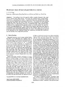
Eq. (8) is valid as an approximation to Eq. (1) when particles are weakly inertial. The vector n is advected in an effective vector field F0 (n) + StF1 (n) that differs from Jeffery’s equation by a term linear in St. This approximation does not capture the formation of caustics that occur when particles with different orientational histories arrive at the same orientation but with different angular velocities [21]. From Eq. (8) we see that the geometrical factor multiplying the inertial correction is 1/αY . Therefore, in the following, we use the effective Stokes number e = St/αY . Solutions to the full equation of motion Eq. (1) are compared to St e We observe solutions of Eq. (8) for a simple shear flow and varying λ and St. that the approximation works well for the examples shown in Fig. 1, although the deviation in panel (d) is discernible. 3. Simple shear flow: stability analysis The simple shear flow, u(r, t) = sy xˆ , is interesting because it is the local linearisation of any flow with parallel streamlines, like pipe flows. It is also the flow in an ideal Couette rheometer used to measure the viscosity of fluids. The solutions of Eq. (8) in the simple shear at St = 0 are a one-parameter family of closed periodic orbits, the well-known Jeffery orbits [5]. The effect of the O(St) terms in 6

(b)

(c)

(d)

Y

Y

(a)

X

X

Figure 1: Numerical solutions of Eq. (1) (red), and Eq. (8) (blue) for four different particles in a e = 0.1; (b) λ = 5, St e = 0.25; (c) λ = 1/5, St e = 0.25; (d) λ = 5, simple shear flow. (a) λ = 1/5, St e St = 0.7. Trajectories on the sphere are shown projected onto a disk with p p the area-preserving Lambert azimuthal stereographic projection X = n x 2/(1 + nz ), Y = ny 2/(1 + nz ) [22]. The grey boundary marks the equator, the blue dot is the initial condition.

7

Figure 2: Simple shear flow and coordinate system.

Eq. (8) is a drift towards a stable periodic orbit. In this section we will characterise this orbit drift for general particle shapes λ by computing the Floquet exponents of the limiting orbits. The modified vector field on the right hand side of Eq. (8) allows for two limiting orbits. First the equatorial orbit, where the n-vector moves in the plane perpendicular to vorticity (usually referred to as tumbling), and second the polar orbit, where the n-vector is fixed parallel to the vorticity (referred to as log rolling). We introduce a spherical coordinate system where θ is the polar angle, measured from the vorticity vector, and ϕ is the azimuthal angle, measured from the flow direction, see Fig. 2. Then the two limiting orbits correspond to θ = 0 and θ = π/2. In spherical coordinates, Eq. (8) takes the following form for a simple shear flow: 1 ϕ˙ = f (θ, ϕ) = (−1 + Λ cos 2ϕ) 2 e StΛ + 2Λ sin2 θ sin 4ϕ + sin 2ϕ((Λ + 1) cos 2θ + Λ − 3) , 8 ˙θ = g(θ, ϕ) = Λ sin θ cos θ sin ϕ cos ϕ e StΛ + sin θ cos θ cos2 (ϕ) 4Λ sin2 θ sin2 ϕ − Λ + 1 . 2 These equations show that inertia induces a coupling between nutation and precession, in contrast with the inertia-free case where the ϕ-dynamics is independent of θ. In the following we denote the limiting periodic orbits ϕ0 (t) and θ0 = 0 8

or π/2. √ The solutions ϕ0 (t) are in both cases periodic with the Jeffery period T = 4π/ 1 − Λ2 . If we introduce arbitrarily small perturbations θ(t) = θ0 + δθ(t) and ϕ(t) = ϕ0 (t) + δϕ(t), then the perturbation δθ(t) evolves according to ∂g ∂g d δθ = δθ + δϕ . dt ∂θ (ϕ0 (t),θ0 ) ∂ϕ (ϕ0 (t),θ0 ) We note that ∂g/∂ϕ = 0 when evaluated at θ = 0 or θ = π/2. This simplification yields ∂g d . (9) ln δθ = dt ∂θ (ϕ0 (t),θ0 ) The Floquet exponent is obtained by time-averaging Eq. (9) along the unperturbed periodic orbit (ϕ0 , θ0 ): Z Z 1 T ∂g 1 2π dϕ ∂g γθ = dt =− . (10) T 0 ∂θ (ϕ0 (t),θ0 ) T 0 ϕ˙ ∂θ (ϕ,θ0 ) The last equality follows from the fact that in one period, ϕ travels monotonically through ϕ = 0 to −2π. Upon evaluating Eq. (10) we obtain for the polar, log rolling orbit γ0 =

e St Λ(1 − Λ) + O(St2 ), 4

and for the equatorial, tumbling orbit γπ/2 =

√ e St (1 − Λ)( 1 − Λ2 − Λ − 1) + O(St2 ). 4

A positive Floquet exponent γ indicates an unstable orbit, and a negative an ate are shown as a function of tracting, stable orbit. The exponents (divided by St) particle shape λ in Fig. 3. We observe that the stable limiting orbit for flat, diskshaped particles is the polar, log rolling orbit, while rod-shaped particles are attracted to the equatorial, tumbling orbit. This is consistent with the intuition that the most stable rotation is that with the mass distributed far from the axis of rotation. Our result explains the orbit drift observed in [15] at small values of St. In Ref. [17] this drift (at small Stokes number and vanishing particle Reynolds number) was explained for nearly spherical particles. Here we generalise the result to arbitrary axisymmetric particles. 9

0.2 e γ/St

0.0

−0.2 −0.4

10−2 10−1

100 λ

101

102

e as functions of aspect ratio λ. Polar orbit, γ0 , in Figure 3: Floquet exponents γ (divided by St) blue, equatorial orbit, γπ/2 , in red.

4. Competition between noise and inertia The indeterminacy of the Jeffery orbits poses a problem for predictions involving the orientational distribution of particles. Jeffery [5] hypothesised that orbits corresponding to minimal energy dissipation should be preferred. Another approach, pursued by a number of authors [23, 24, 6], shows that thermal noise, after a long time, removes the dependence on initial conditions and produces a stationary distribution of the n vector. In particular, in [24] it is shown that the orientational distribution converges to a function independent of noise strength, as the noise strength is reduced. On the contrary, in the preceding sections we have shown that in the absence of noise a weakly inertial particle will rotate into a specific stable orbit. In this section we consider what effect weak particle inertia have on the orientational distribution. The time scale for inertia to have an effect is equal to the inverse Floquet expoe The corresponding time scale for diffusion is sτD ∼ Pe, where nent, s/γ ∼ 1/St. the Péclet number Pe = s/D measures the noise strength, or diffusion constant e 1 we eC , relative to the shear strength [20]. Thus, when τD γ ∼ PeSt D = kB T/Y expect noise to determine the stationary distribution, as described by previous aue 1 we expect a distribution dominated thors [6]. On the other hand, when PeSt by the inertial effects, with a peak around the stable orbit described in the previous section. In order to quantify these expectations we need to compute moments of e and λ. the stationary distribution for various Pe, St The Fokker-Planck equation describing the evolution of the orientational prob-

10

ability density P(n, t) is ˆ ∂t P(n, t) = −∂ n [(F0 (n) + StF1 (n))P] + Pe−1 ∂2nP ≡ JP.

(11)

Here ∂ n is the gradient on the sphere defined as ∂ n ≡ (I − nnT )∇. The boundary condition of Eq. (11) is that the probability density P must integrate to unity over the sphere. The Fokker-Planck equation can be solved numerically by expansion in spherical harmonics, the details of this procedure are described in Appendix A. For a discussion of the solutions of Eq. (11) we compute the stationary average hsin2 θi, where θ is the polar angle from the vorticity vector of the simple shear flow (see Fig. 2). Recall that weakly inertial rod-shaped particles exhibit a stable orbit at θ = π/2, and disk-shaped particles at θ = 0. Moreover, values of hsin2 θi have been tabulated (Table 6c in Ref. [6]) for different values of Pe and λ. This allows us to validate our method at St = 0. In Fig. 4 we show the angular average hsin2 θi as a function of Pe for different values of St, and for two particle shapes: prolate λ = 5 and oblate λ = 1/5. We note the following features. At strong noise, that is small Pe, the moment is independent of St and approaches the uniformly random result hsin2 θi = 2/3. Next we see that the curve for St = 0 (red curve) levels out and converges at a finite value of Pe, as predicted in Ref. [24]. Finally we see that for finite St, the curves coincide with the St = 0 curve up to PeSt ≈ 1, but then deviates and instead converges towards hsin2 θi = 1 (prolate particle), or hsin2 θi = 0 (oblate particle) when PeSt 1. The limit of St → 0 is singular: the stationary distribution at low noise and weak inertia differs substantially from the one predicted by a St = 0 calculation, although the time to arrive at the steady state becomes longer for weaker inertia. The most important observation is that the stationary average at low noise strength but without inertia is the same for prolate and oblate particles, whereas the inertial correction has opposite directions for the two different shapes. We emphasise this e observation in Fig. 5, where we show the stationary average as function of PeSt, e e for different values of St/Pe. It turns out that when PeSt is large enough, then the e and Pe separately, but only in the combination PeSt. e average does not depend on St e The stationary average is determined by the ratio of relaxation times τD γ ∼ PeSt, e and by the aspect ratio λ. For small values of PeSt the stationary distribution is instead determined by Pe, as shown in Fig. 4.

11

0.9 0.8 hsin2 θi

0.7 0.6 0.5 0.4 100 101 102 103 104 105 106 107 Pe

e and λ. Solid lines are Figure 4: Stationary orientational average as function of Pe for different St e = 0 result, then blue a prolate particle λ = 5, dashed lines oblate λ = 1/5. The red solid line is St e = 10−4 , green St e = 10−3 , purple St e = 10−2 and orange St e = 10−1 . St

0.9 0.8 hsin2 θi

0.7 0.6 0.5 0.4 10−6 10−4 10−2 100 e PeSt

102

e for different values of k = St/Pe. e Figure 5: Stationary orientational average as function of PeSt −9 Solid lines are a prolate particle λ = 5, dashed lines oblate λ = 1/5. Then red k = 10 , blue k = 10−8 , green k = 10−7 , purple k = 10−6 and orange k = 10−5 .

12

5. Conclusions The orientational dynamics of weakly inertial axisymmetric particles in a steady flow has been investigated. We have derived an approximate equation of motion for the unit axial vector along the particle symmetry axis, assuming that the Stokes number is small. The fact that we have obtained this equation of motion in explicit form (valid for any axisymmetric and weakly inertial particle in any steady linear viscous flow) has made it possible to address two important questions, both pertaining to the case of a simple shear flow. First, we have shown that axisymmetric particles drift towards either the logrolling (disk-shaped particles) or the tumbling orbit (rod-like particles). We have quantified this result for any particle aspect ratio by calculating the Floquet exponents of the periodic orbits to leading order in St. Our result generalises a result for nearly spherical particles in Ref. [17] to arbitrary axisymmetric particles. Second, the approximate equation of motion derived in Sec. 2 has allowed us to formulate the Fokker-Planck equation describing the orientational distribution of axisymmetric, weakly inertial particles in a shear flow when rotational noise is present. Numerical solutions of the Fokker-Planck equation show that statione 1, ary orientational distributions are close to the inertia-free case when PeSt e whereas they are determined by inertial effects, though small, when Pe 1/St 1. An important open question is to describe the effect of fluid inertia (at small but finite particle Reynolds number) upon the orientational motion for particles with arbitrary aspect ratios, in competition with the effects of particle inertia and rotational noise. The calculations summarised in this article are restricted to axisymmetric particles. But our approach is readily generalised to asymmetric (triaxial) particles. Acknowledgements Financial support by Vetenskapsrådet, by the Göran Gustafsson Foundation for Research in Natural Sciences and Medicine, and by the EU COST Action MP0806 on ‘Particles in Turbulence’ are gratefully acknowledged. References [1] C. Rolf, M. Kramer, C. Schiller, M. Hildebrandt, M. Riese, Lidar observation and model simulation of a volcanic-ash-induced cirrus cloud during the 13

Eyjafjallajökull eruption, Atmos. Chem. Phys. Discuss. 12 (2012) 15675– 15707. [2] H. Stommel, Trajectories of small bodies sinking slowly through convection cells., J. Marine Res. 8 (1949) 24–29. [3] J. S. Guasto, R. Rusconi, R. Stocker, Fluid mechanics of planktonic microorganisms, Annual Review of Fluid Mechanics 44 (1) (2012) 373–400. [4] F. Lundell, L. D. Söderberg, P. H. Alfredsson, Fluid mechanics of papermaking, Annual Review of Fluid Mechanics 43 (1) (2011) 195–217. [5] G. B. Jeffery, The motion of ellipsoidal particles immersed in a viscous fluid, Proceedings of the Royal Society of London Series A 102 (715) (1922) 161– 179. [6] H. Brenner, Rheology of a dilute suspension of axisymmetric Brownian particles, International Journal of Multiphase Flow 1 (2) (1974) 195–341. [7] C. J. Petrie, The rheology of fibre suspensions, Journal of Non-Newtonian Fluid Mechanics 87 (2–3) (1999) 369–402. [8] G. Gauthier, P. Gondret, M. Rabaud, Motions of anisotropic particles: Application to visualization of three-dimensional flows, Phys. Fluids 10 (9) (1998) 2147–2154. [9] M. Wilkinson, V. Bezuglyy, B. Mehlig, Fingerprints of random flows?, Physics of Fluids 21 (4) (2009) 043304. [10] M. Wilkinson, V. Bezuglyy, B. Mehlig, Emergent order in rheoscopic swirls, Journal of Fluid Mechanics 667 (2011) 158–187. [11] V. Bezuglyy, B. Mehlig, M. Wilkinson, Poincaré indices of rheoscopic visualisations, Europhysics Letters 89 (2010) 34003. [12] J. Einarsson, A. Johansson, S. K. Mahato, Y. Mishra, J. R. Angilella, D. Hanstorp, B. Mehlig, Periodic and aperiodic tumbling of microrods advected in a microchannel flow, Acta Mechanica, in press (2013). [13] A. Pumir, M. Wilkinson, Orientation statistics of small particles in turbulence, New Journal of Physics 13 (9) (2011) 093030. 14

[14] S. Parsa, E. Calzavarini, F. Toschi, G. A. Voth, Rotation rate of rods in turbulent fluid flow, Physical Review Letters 109 (2012) 134501. [15] F. Lundell, A. Carlsson, Heavy ellipsoids in creeping shear flow: Transitions of the particle rotation rate and orbit shape, Phys. Rev. E 81 (2010) 016323. [16] F. Lundell, The effect of particle inertia on triaxial ellipsoids in creeping shear: From drift toward chaos to a single periodic solution, Phys. Fluids 23 (2011) 011704. [17] G. Subramanian, D. L. Koch, Inertial effects on the orientation of nearly spherical particles in simple shear flow, Journal of Fluid Mechanics 557 (2006) 257–296. [18] P. M. Lovalenti, J. F. Brady, The hydrodynamic force on a rigid particle undergoing arbitrary time-dependent motion at small reynolds number, Journal of Fluid Mechanics 256 (1993) 561–605. [19] C. Marchioli, M. Fantoni, A. Soldati, Orientation, distribution, and deposition of elongated, inertial fibers in turbulent channel flow, Physics of Fluids 22 (3) (2010) 033301. [20] S. Kim, S. Karrila, Microhydrodynamics: Principles And Selected Applications, Butterworth - Heinemann series in Chemical Engineering, 1991. [21] K. Gustavsson, J. Einarsson, B. Mehlig, Tumbling of small axisymmetric particles in random and turbulent flows, arXiv e-print 1305.1822 (2013). [22] J. P. Snyder, Map Projections: A Working Manual, Geological Survey (U.S.), 1987. http://pubs.er.usgs.gov/publication/pp1395. [23] H. A. Scheraga, Non–Newtonian viscosity of solutions of ellipsoidal particles, The Journal of Chemical Physics 23 (8) (1955) 1526–1532. [24] E. J. Hinch, L. G. Leal, The effect of Brownian motion on the rheological properties of a suspension of non-spherical particles, Journal of Fluid Mechanics 52 (04) (1972) 683–712. [25] G. Arfken, Mathematical Methods for Physicists, Second Edition, Academic Press, 1970.

15

[26] J. J. Sakurai, S. F. Tuan (ed.), Modern quantum mechanics, Addison-Wesley Pub. 1994. [27] https://github.com/jeinarsson/fpe_sphere.

16

Appendix A. Solution of the Fokker-Planck equation We start from the Fokker-Planck equation governing the evolution of the probability density P(n, t) of finding a particle with orientation vector n at time t: ˆ ∂t P(n, t) = −∂ n [ n˙ P] + Pe−1 ∂2nP ≡ JP with the normalisation condition Z dn P(n, t) = 1.

(A.1)

(A.2)

S2

The differential operator ∂ n is the gradient on the sphere, defined by taking the usual gradient ∇ in R3 projected onto the unit sphere, ∂ n ≡ (I − nnT )∇. The drift term n˙ may be any polynomial function of n, for example the equation of motion Eq. (8). We approximate the solution of Eq. (A.1) by an expansion in spherical harmonics [23], the eigenfunctions of the quantum-mechanical angular-momentum operators, which form a complete basis on S 2 . We use bra-ket notation, P(n, t) = hn|P(t)i =

∞ X l X

cml (t)hn|l, mi

(A.3)

l=0 m=−l

where s hn|l, mi = Ylm (n) = (−1)m

2l + 1 (l − m)! m P (cos θ)eimϕ . 4π (l + m)! l

(A.4)

We use the standard spherical harmonics defined in for example [25] (p. 571). The functions Pml are the associated Legendre polynomials. We call the timedependent coefficients for each basis function cml (t), and the fact that P is realvalued constrains the coefficients: c−m = (−1)m cml , l

(A.5)

where the bar denotes complex conjugation. Then Eq. (A.1) for the time evolution of the state |P(t)i reads d ˆ |P(t)i = J|P(t)i . dt 17

Inserting the expansion yields l l ∞ X ∞ X X X d m ˆ mi. cml (t) J|l, cl (t)|l, mi = dt l=0 m=−l l=0 m=−l

(A.6)

Multiplying with hp, q|, and using the orthogonality of the spherical harmonics we arrive at a system of coupled ordinary differential equations for the coefficients cml (t) c˙ qp (t) =

l ∞ X X

ˆ mi, cml (t)hp, q| J|l,

(A.7)

l=0 m=−l

1 c00 = √ . 4π

(A.8)

In order to solve Eq. (A.7) it remains to compute the matrix elements of the operaˆ This is achieved by expressing Jˆ as a combination of the angular momentum tor J. operators. How the angular momentum operators act on the spherical harmonics is well known, see for example Ref. [25]. The angular momentum operator Lˆ is given by Lˆ = −i nˆ ∧ ∇. In terms of Lˆ we have 2 ∂2n = (I − nˆ nˆ T )∇ · (I − nˆ nˆ T )∇ = − Lˆ ,

and ˆ ∂ n = (I − nˆ nˆ T )∇ = −i nˆ ∧ L. 2 The states |l, mi are the eigenfunctions of Lˆ and Lˆ 3 with eigenvalues l(l + 1) and m. Now, to evaluate the drift term ∂ n n˙ we need to know how Lˆ 1 , Lˆ 2 , and nˆ act on |l, mi. The first two are known through the use of ladder operators, defined by

1 Lˆ ± = Lˆ 1 ± iLˆ 2 =⇒ Lˆ 1 = (Lˆ + + Lˆ − ), 2

i Lˆ 2 = − (Lˆ + − Lˆ − ) 2

and their effect is Lˆ ± |l, mi =

p

(l ∓ m)(1 + l ± m) |l, m ± 1i. 18

Next, the drift term we consider is a polynomial in nˆ 1 , nˆ 2 and nˆ 3 (the components of nˆ ), we therefore need to evaluate the action of a monomial nˆ α1 nˆ β2 nˆ γ3 on |l, mi. Any such monomial of order k = α + β + γ may be written as a linear combination of spherical tensor operators of up to order k: nˆ α1 nˆ β2 nˆ γ3 =

k X l X

aml (α, β, γ)Yˆ lm .

l=0 m=−l

The action of Yˆ pq is computed with the Clebsch-Gordan coefficients (see for example Ref. [26], p.216) Yˆ pq |l, mi =

p X

K(p, q, l, m, l + ∆l, m + q)|l + ∆l, m + qi,

∆l=−p

where s K(l1 , m1 , l2 , m2 , l, m) =

(2l1 + 1)(2l2 + 1) 4π(2l + 1)

× hl1 l2 ; 00|l1 l2 ; l0ihl1 l2 ; m1 m2 |l1 l2 ; lmi . The Clebsch-Gordan coefficients are denoted by hl1 l2 ; m1 m2 |l1 l2 ; lmi (see e.g Eq. (3.7.44) of Ref. [26]), and they are available in Mathematica by the function ClebschGordan[l1,m1,l2,m2,l,m]. Finally, we order the operators, so that as many terms as possible cancel before we actually begin evaluating the operators. In particular we want to reorder nˆ i against Lˆ i , and we make use of the commutator [ˆn p , Lˆ q ] =

3 X

iε pq j nˆ j ,

j=1

where εi jk is the Levi-Civita tensor. Let us consider an example. In the special case of Jˆ = Pe−1 ∂2n we see that 2 Jˆ = −Pe−1 Lˆ . It follows: ˆ mi = −Pe−1 Lˆ 2 |l, mi = −l(l + 1)Pe−1 |l, mi. J|l, Knowing how Jˆ acts on |l, mi fully specifies Eq. (A.7) which becomes c˙ qp (t) = −p(p + 1)Pe−1 cqp (t). 19

This means that the diffusion operator exponentially suppresses all modes with p > 0, and the lowest mode p = 0 is determined by the normalisation condition Eq. (A.8). This is the solution of the diffusion equation on the sphere, with the uniform distribution as steady state. Now take the for the drift term the standard Jeffery equation n˙ = On + Λ(Sn − T nn Sn) = F0 (n), and call this operator Jˆ = −∂ n F0 (n) + Pe−1 ∂2n. We find r r r π π π ˆ ˆ1 ΛLˆ − Yˆ 2−1 + i Lˆ − Yˆ 21 − i ΛL+ Y2 Jˆ = i 30 30 30 r r r π ˆ ˆ −1 2π ˆ ˆ −2 2π ˆ ˆ 2 −i ΛL3 Y2 − i ΛL3 Y2 L+ Y2 − i 30 15 15 r 2 √ ˆ ˆ0 2 π ˆ ˆ0 2 + i πL3 Y0 − i L3 Y2 − Pe−1 Lˆ . 3 3 5 The fact that the operator Jˆ is real implies that the matrix elements must have the symmetry ˆ mi = (−1)q hp, −q| J|l, ˆ mi. hp, q| J|l, We can understand the reason for this because the system of differential equations in Eq. (A.7) needs to preserve the condition that P is real, as stated in Eq. (A.5). It implies we have only to compute half of the matrix elements. Upon including the correction Eq. (8) due to weak particle inertia, the expression for the operator Jˆ becomes too lengthy to include here. However, we have implemented the identities and rules described in this appendix in a Mathematica ˆ it converts the notebook [27]. Given an operator Jˆ expressed in terms of nˆ and L, expression into sums of angular momentum operators as exemplified above. We also provide an additional Mathematica notebook that, given the matrix elements, assembles a sparse matrix J, up to a desired order lmax . This matrix can then be used to solve the truncated version of Eq. (A.7): c˙ = Jc, where c is a vector with elements cml . Alternatively, the matrix can be solved for the stationary solution of c. All results shown in this paper were computed using lmax = 400, which leads to very good convergence in all cases shown. Only when solutions approach delta peaks, as for example the limiting stable orbits in the large PeSt case, the expansion procedure converges very slowly. 20