Origin of Power-Law Spatial Correlations in Distributed Oscillators and

VOLUME 76, NUMBER 23

PHYSICAL REVIEW LETTERS

3 JUNE 1996

Origin of Power-Law Spatial Correlations in Distributed Oscillators and Maps with Nonlocal Coupling Yoshiki Kuramoto and Hiroya Nakao Department of Physics, Graduate School of Sciences, Kyoto University, Kyoto 606, Japan (Received 4 March 1996) It is argued that power-law spatial correlation at short distances is a generic property of spatiotemporal chaos exhibited by active dynamical elements coupled nonlocally. While this fact was suggested earlier from some numerical analysis of coupled limit cycles, further evidence is provided here from an analysis for chaotic Rössler oscillators and logistic maps. A theory is presented to explain why such short-range nonanalyticity of correlation with parameter-dependent exponent is so universal when the coupling is nonlocal. [S0031-9007(96)00359-6] PACS numbers: 05.45.+b, 47.53.+n

Existing theories on extended fields or large assemblies of active dynamical elements [1] usually assume local coupling or otherwise global coupling, while the studies associated with nonlocal finite-range coupling are relatively few. A typical model for the latter class of systems with a set of field variables Asr, td has the form ≠A ­ FsAd 1 B . ≠t

(1)

Here FsAd represents the vector field of a dynamical element (limit cycle, chaotic oscillator, excitable unit, etc.) at site r. The elements are Rnow under the control of a self-generated field Bsr, td ; ssr ˆ 2 r 0 dAsr 0 , tddr 0 , where sˆ is a nonlocal coupling matrix. Although the elements are supposed in (1) to form a quasicontinuous distribution, spatial continuity of the field amplitude itself will no longer be guaranteed once the coupling becomes nonlocal. The term “nonlocal coupling” need not be taken literally, because this form of coupling may result, e.g., from adiabatic elimination of rapidly diffusing components in systems of diffusion coupling, i.e., a typical local coupling [2–4]. Consider the case that each dynamical element represents a small-amplitude oscillator near a supercritical Hopf bifurcation. Then the center-manifold reduction of (1) leads to a complex Ginzburg-Landau (CGL) type equation with nonlocal coupling [4]. It has the canonical form

coupling range has been taken to be the length unit. In all systems studied below, periodic boundary conditions with period L ¿ 1 will be assumed. The other extreme L ø 1 gives global coupling. The latter idealization has been instrumental in developing some important notions such as synchronization transition [5–7], clustering [8–11], and collective chaos [12,13]. Local-coupling approximation (LCA) of (2) is valid when W is sufficiently long waved, and this leads to the standard CGL equation. Uniform oscillation W ­ exps2ic2 td, which satisfies (2) and its LCA, becomes unstable when 1 1 c1 c2 , 0, giving rise to turbulence in both cases. Uniqueness of the turbulence in the nonlocal CGL (2) manifests itself under such strong instability that short-scale turbulent fluctuations come to invade the domain inside the range of coupling. Since no characteristic length exists below the coupling range down to the “atomic” scale, the turbulence here bears some resemblance to the developed fluid turbulence in the inertial subrange. We now summarize our previous findings [2–4] on this type of turbulence. Define spatial correlation Gsxd ­ kXs0dXsxd 1 Y s0dYsxdl and related quantity gsxd ; Gs0d 2 Gsxd, where k· · ·l stands for a long-time average. Our numerical analyses of (2) proved the existence of an open parameter range in which gsxd for x ø 1 has the nonanalytic form gsxd ­ g0 1 g1 x a ,

sx fi 0d ,

(3)

where W is a complex field with the real and imaginary parts denoted by X and Y , respectively, and Z represents the internal field. The following discussion will be restricted to one-dimensional systems. Assuming exponential coupling, which is appropriate for the diffusionmediated coupling Rmentioned in the last paragraph [2], we 1 ` have Zsx, td ­ 2 2` exps2jx 2 x 0 jdW sx 0 , td dx 0 . The

where g0 , g1 , and a are nonnegative constants. g0 is nonvanishing only below a certain coupling strength Kc sc1 , c2 d. Since gs0d ­ 0 by definition, nonvanishing g0 implies a discontinuity in G at x ­ 0. Physically, this signifies individual motions or disintegration of the amplitude profile into its microscopic constituents. Remarkably, the exponent a varies with K. Near Kc , a is definitely less than 1, so that the peak of Gsxd is cusped then. If 0 , a , 1 and g0 ­ 0, then we have a continuous but fractal amplitude profile of dimension Df , and the relation Df ­ 2 2 a is suggested numerically. The case a ­ 1 does not still give a simple 1D profile, but the measured length diverges logarithmically as the

4352

© 1996 The American Physical Society

≠W ­ W 2 s1 1 ic2 djW j2 W 1 Ks1 1 ic1 d sZ 2 Wd , ≠t (2)

0031-9007y96y76(23)y4352(4)$10.00

VOLUME 76, NUMBER 23

PHYSICAL REVIEW LETTERS

minimum scale of measurement tends to zero. All these results remain qualitatively the same when the oscillator type is changed to the Brusselator [3]. The main goal of this Letter is to present a theory to explain all these findings. Before doing this, however, we show briefly how one may even replace the limit cycles with chaotic oscillators or maps to obtain essentially the same results. Consider a quasicontinuous array of chaotic Rössler oscillators with exponential coupling dXydt ­ 2Y 1 Z 1 Ksj 2 Xd , dY ydt ­ X 1 0.3Y 1 Ksh 2 Y d , dZydt ­ 0.2 1 XZ 2 5.7Z 1 Ksz 2 Zd , 1

(4)

R

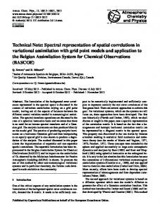
where jsxd ­ 2 exps2jx 2 x 0 jdXsx 0 d dx 0 ; h and z are similarly defined in terms of Y and Z, respectively. With the parameter values assumed, the individual Rössler oscillator gives a funnel attractor. Some characteristic profiles of the spatial correlation Gsxd ; kXs0dXsxdl are displayed in Fig. 1. The sharpness of the correlation peak changes with the coupling strength K, and its jump at x ­ 0 appears for weaker coupling. These are the features already seen for the model (2) [2–4]. Figure 2 demonstrates the power law of gsxd with a changing with K, where we employed the previous method [2] for estimating g0 and a. It is difficult to locate Kc accurately, and our rough estimation gives Kc ­ ,0.14 0.15. We also studied exponentially coupled logistic maps

FIG. 1. Some correlation profiles obtained numerically from an array of 4096 Rössler oscillators (4) with L ­ 16. The peak position Gs0d is indicated by an arrow in (a) and (b).

3 JUNE 1996

Xn11 ­ fsXn d 1 Kfhn 2 fsXn dg ,

(5)

1 R where fsXd ­ 3.7Xs1 2 Xd and hn sxd ­ 2 exps2jx 2 x 0 jdffXn sx 0 dg dx 0 . Figure 3 confirms that gsxd obeys a power law again. The correlation jump at x ­ 0 appears below K . 0.24. Although not shown here with data, fractal amplitude profiles with the dimension Df . 2 2 a has been confirmed both for Rössler oscillators and logistic maps. Aforementioned logarithmic singularity at about a ­ 1 has also proved to be a common feature. Although power-law spatial correlations may naturally be understood as a characteristic of those fluctuations which occur in a scaleless regime, this fact alone cannot lead us to the understanding of the more specific aspects of the phenomenon. In presenting our theory below, we shall use terminology appropriate for differential-equation models like (1). Still the underlying physics may apply to coupled maps as well. Equation (1) describes a single forced oscillator (limit cycle or chaotic) if we regard Bstd as a given timedependent quantity. One may then define space-time local Lyapunov exponent lstd associated with each oscillator. l will fluctuate with B, and may alternate its sign irregularly. Imagine a pair of oscillators with mutual distance x ø 1, and assume that they share common lstd. The latter is true if their amplitude difference ysxd ; Asxd 2 As0d remains sufficiently small. Obviously, we 1 have gsxd ­ 2 kj yj2 l, where the correlation has been defined by Gsxd ­ kAs0dAsxdl. Suppose at first that lstd never becomes positive. Then the oscillators will synchronize with the motion of B. The latter should be a smooth function of x with characteristic length of Os1d because its definition involves a spatial average over the distance of Os1d. Thus A will also behave smoothly in space, implying jysxdj ~ x or gsxd ~ x 2 yielding a normal correlation. In a different parameter regime, lstd may occasionally become positive. Suppose that an unstable phase [lstd . 0] has been initiated after a long duration of stable phase [lstd , 0]. Initially we have jyj ­ Osxd, but this small

FIG. 2. gsxd 2 g0 vs x in logarithmic scales for different coupling strengths. They are obtained numerically from an array of 4096 Rössler oscillators (4) with L ­ 16.

4353

VOLUME 76, NUMBER 23

PHYSICAL REVIEW LETTERS

3 JUNE 1996

ˆ is replaced with lstd. Assume of y. Concomitantly, Lstd further that the effect of N is basically to suppress the unstable growth of y. Similarly, the principal role of D term will be to keep y away from the zero value in the decaying phase. These effects may be incorporated by introducing “hard walls” at y ­ y0 and D ; bstdx. By neglecting the t dependence of b, the walls may be set at y ­ 1 and x in suitable scales of y and x. Our equation thus becomes

FIG. 3. gsxd 2 g0 vs x in logarithmic scales for different coupling strengths. They are obtained numerically from an array of 4096 logistic maps (5) with L ­ 16.

quantity will grow exponentially. Suppose further that as a result of this unstable growth having continued for time t, jyj has become Os1d, i.e., some value independent of x. Then we have tsxd ~ jlnxj, which is a large number for sufficiently small x. Thus there may be little chance for such an event to occur. Still such rare events may contribute to kjyj2 l more significantly than the normal contribution of Osx 2 d. The former contribution should be proportional to the probability that the duration of a given unstable phase be longer than tsxd. If lstd forms a Markoffian random process in long time scales, which we assume, this probability will be exponentially small like exps2btd for large t. Thus gsxd ~ Psxd ~ exps2btd ~ x a ,

(6)

where a and b are some positive constants. This gives a rough sketch of how power-law spatial correlations arise. The above reasoning, being based on some vaguely defined notions, is admittedly too crude, and is also unable to explain the origin of the correlation jump. What is intended here, however, is only to suggest that the power law may result from a miraculous combination of two exponential functions of different physical origins, one associated with a Markoffian random process and the other with the dynamics of unstable growth [14]. To make the argument more quantitative, we now try to derive an approximate equation for y to calculate kj yj2 l. The equation for y obtained from (1) generally takes the form dy ˆ ­ Lstdy 1 Ns yd 1 Dsx, td , dt

(7)

ˆ where Lstdy is the linearization of FsAd about A ­ As0, td; Ns yd represents nonlinear terms, and D gives the difference in the internal field between the two oscillators; i.e., Dsx, td ­ Bsx, td 2 Bs0, td . bstdx with randomly fluctuating bstd. Some drastic approximations on (7) are now made. First, we replace y with a scalar y, by which we are keeping track only of the most unstable component 4354

dy ­ lstdy 1 e 21 f2us y 2 1d 1 usx 2 ydg, dt e °! 01 , (8) where u denotes the Heaviside step function. Finally, we simplify the random process of lstd by assuming that lstd takes only two values l1 and 2l2 (l1,2 . 0) and that the transitions 2l2 ! l1 and l1 ! 2l2 occur with nonzero probabilities p and q, respectively. The average Lyapunov exponent thus becomes l ­ sl1 p 2 l2 qdysp 1 qd. Fortunately, the above model can be solved exactly for the stationary distribution rs syd and hence k y 2 l. It seems useful here to notice that the statistical ensemble of our system is equivalent to an ideal two-component gas, where the particles of one type are accelerated and the other type decelerated exponentially between the two walls, while the particle types themselves will also be interchanged spontaneously; a particle having reached one of the walls will stay there until its type is changed. We will consider only the case l1 ­ l2 ­ 1 below because there is nothing qualitatively new about more general cases. Let the normalized density rs y, td be expressed as rs y, td ­ r1 s y, td 1 r2 s y, td 1 R1 stdds y 2 1d 1 R2 stdds y 2 xd , (9) where r6 are the densities between the walls, the suffixes 1 and 2 specifying components with positive and negative l, respectively, and singular contributions from the walls have been separated out as the last two terms. Then the respective parts of the distribution are governed by ≠r1 y≠t ­ 2≠s yr1 dy≠y 2 qr1 1 pr2 , ≠r2 y≠t ­ ≠s yr2 dy≠y 1 qr1 2 pr2 , dR1 ydt ­ r1 s1d 2 qR1 , (10) dR2 ydt ­ xr2 sxd 2 pR2 . R R Demanding qs r1 dy 1 R1 d ­ ps r2 dy 1 R2 d, which assures the net balance between the two species, we find rs s yd ­

l f2pqy 211p2q p 2 qx p2q 1 pds y 2 1d 1 qx p2q ds y 2 xdg,

sp fi qd (11)

VOLUME 76, NUMBER 23

PHYSICAL REVIEW LETTERS

from which kjyj2 l and hence gsxd are calculated: gsxd ­

(III0 ) q 2 p ­ 1 (i.e., a ­ 1):

l 2s2 1 p 2 qd ps2 1 p 1 qd 1 qs2 2 p 2 qdx 21p2q . 3 p 2 qx p2q (12)

For sufficiently small x, gsxd has the following asymptotic forms depending on the parameter range concerned: (I) q . p si.e., l , 0d: gsxd ­

jlj fps2 1 p 1 qdx q2p 1 qs2 2 p 2 qdx 2 g . 2qs2 1 p 2 qd (13)

Thus gsxd , x 2 if q . p 1 2, giving a normal correlation profile, while gsxd , x a if p , q , p 1 2, where a ­ q 2 p so that 0 , a , 2. (II) p . q si.e., l . 0d: gsxd ­

ls2 1 p 1 qd sp 1 qx p2q d . 2ps2 1 p 2 qd

(14)

This has the expected form gsxd ­ g0 1 g1 x a with nonvanishing g0 and a ­ p 2 q . 0. Near p ­ q (or l ­ 0), we have another asymptotic regime in which x is kept small and finite while p 2 q tends to 0. Specifically, (III) jsp 2 qd lnxj ø 1: gsxd ­

11p . 4pjlnxj

ps1 1 p 1 qdx q2p 1 qs1 2 p 2 qdx . qs1 1 p 2 qd (16)

Thus we have k yl , x and hence Df ­ 1 if q . p 1 1, while k yl , x a with a ­ q 2 p and hence Df ­ 2 2 a if p , q , p 1 1 (i.e., 0 , a , 1). (II) p . q: k yl ­ and hence Df ­ 2.

ls1 1 p 1 qd , 11p2q

k yl ­ 22pjljx lnx ,

(18)

and hence Ssxd , jlnxj. The expected relation Df ­ 2 2 a has thus been confirmed, and the logarithmic singularity at a ­ 1 has also been explained. For all its remarkable success, our theory leaves some problems yet to be resolved. Contrary to the theory, there is no indication from our numerical analysis so far that a vanishes at any value of K. Furthermore, l seems to remain negative even after the appearance of a discontinuity in G. More careful numerical analysis seems necessary especially near the onset of individual motions where some interference from the asymptotic regime (III) is implied from the theory. Finally, the present theory suggests that the anomalous behavior of fluctuations discussed so far depends neither on the spatial dimension of the system nor on the detailed functional form of the coupling. It seems even irrelevant that the origin of the random forcing B be the mutual coupling of the elements. The authors thank T. Mizuguchi and S. Kitsunezaki for fruitful discussions. The present work has been supported by the Japanese Grand-in-Aid for Science Research Fund from the Ministry of Education, Science and Culture (No. 07243106).

(15)

We have thus succeeded in reproducing both the powerlaw correlations with parameter-dependent a and the transition associated with the appearance of a correlation jump. Fractal amplitude profiles can also be derived. Let the measured length of a segment of an amplitude profile over the unit interval be Ssxd, where x indicates the minimum scale of measurement. By definition, Ssxd , x 12Df , while Ssxd . k ylyx if the sum of the amplitude differences y dominates Ssxd (which is the case if Ssxd ! ` as x ! 0). Df is then estimated for three characteristic regimes as follows: (I) q . p, q 2 p fi 1 (i.e., a fi 1): k yl ­ jlj

3 JUNE 1996

(17)

[1] For a review, see M. C. Cross and P. C. Hohenberg, Rev. Mod. Phys. 65, 851 (1993). [2] Y. Kuramoto, Prog. Theor. Phys. 94, 321 (1995). [3] Y. Kuramoto and H. Nakao, Physica D (to be published). [4] Y. Kuramoto, Int. J. Bif. Chaos (to be published). [5] A. T. Winfree, J. Theor. Biol. 16, 15 (1967). [6] Y. Kuramoto, in Proceedings of the International Symposium on Mathematical Problems in Theoretical Physics, edited by H. Araki, Lecture Notes in Physics Vol. 39 (Springer, Berlin, 1975); Chemical Oscillations, Waves, and Turbulence (Springer, Berlin, 1984). [7] K. Wiesenfeld, P. Colet, and S. Strogatz, Phys. Rev. Lett. 76, 404 (1996). [8] K. Kaneko, Physica (Amsterdam) 54D, 137 (1990). [9] D. Golomb, D. Hansel, B. Shraiman, and H. Sompolinsky, Phys. Rev. A 45, 3516 (1992). [10] K. Okuda, Physica (Amsterdam) 63D, 424 (1993). [11] S. K. Han, C. Kurrer, and Y. Kuramoto, Phys. Rev. Lett. 75, 3190 (1995). [12] V. Hakim and W. J. Rappel, Phys. Rev. A 46, R7347 (1992). [13] N. Nakagawa and Y. Kuramoto, Prog. Theor. Phys. 89, 313 (1993); Physica (Amsterdam) 80D, 307 (1995). [14] Power-law behavior resulting from a combination of two exponentially changing processes was also noticed by E. Fermi [Phys. Rev. 75, 1169 (1949)] in his theory on the energy spectrum of the cosmic radiation. The authors thank V. Hakim for pointing out this coincidence.

4355