Traditionally, each multi-dimensional data item is represented as a vector. ..... blocks stored on the hard disks so that each block can fit into the main memory of a ...
To appear in ACM Transactions on Graphics (Special Issue of SIGGRAPH 2005)
Out-of-Core Tensor Approximation of Multi-Dimensional Matrices of Visual Data Hongcheng Wang
Qing Wu
Lin Shi
Yizhou Yu
Narendra Ahuja
University of Illinois at Urbana-Champaign
Abstract Tensor approximation is necessary to obtain compact multilinear models for multi-dimensional visual datasets. Traditionally, each multi-dimensional data item is represented as a vector. Such a scheme flattens the data and partially destroys the internal structures established throughout the multiple dimensions. In this paper, we retain the original dimensionality of the data items to more effectively exploit existing spatial redundancy and allow more efficient computation. Since the size of visual datasets can easily exceed the memory capacity of a single machine, we also present an outof-core algorithm for higher-order tensor approximation. The basic idea is to partition a tensor into smaller blocks and perform tensorrelated operations blockwise. We have successfully applied our techniques to three graphics-related data-driven models, including 6D bidirectional texture functions, 7D dynamic BTFs and 4D volume simulation sequences. Experimental results indicate that our techniques can not only process out-of-core data, but also achieve higher compression ratios and quality than previous methods.
Figure 1: A virtual scene with a cube mapped with a SPONGE BTF and a vase mapped with a LICHEN BTF. There is a point light source near the ”sponge”.
CR Categories: I.3.3 [Computer Graphics]: Picture/Image Generation; I.3.7 [Computer Graphics]: Three-dimensional Graphics and Realism—color, shading, shadowing, and texture
subsequent tensor approximation. Such a strategy is actually suboptimal because it ignores the large amount of redundancy due to spatial coherence within every multi-dimensional data item. This is obvious for images as adjacent rows or columns of an image often exhibit similar color patterns. In this paper, we propose to formulate higher-order tensors to exploit spatial coherence available in individual multi-dimensional data items, such as 2D images and 3D volumes. As a result, subsequent tensor approximation can also remove the spatial redundancy in these data and give rise to a much more compact representation. Since the most important motivation of tensor approximation is to produce a compact representation from a huge amount of redundant data, it becomes particularly meaningful when the original data cannot fit into the main memory of a single machine. Virtual memory cannot help much because the largest possible (virtual) memory capacity of a computer with a 32-bit architecture is only around 4GB and multi-dimensional datasets larger than that are not uncommon. Out-of-core processing capability is therefore much desired. Such a technique is useful even when the virtual memory allows addressing of the entire data but, in practice, the small physical memory will cause extensive swapping. Typically, application-specific data partitioning and swapping can give far better performance. We present an efficient out-of-core algorithm for tensor approximation. It is based on a simple block-based partition. With such an algorithm, we are able to process datasets larger than 10GB on a PC with less than 1GB memory. We have successfully applied our new tensor approximation techniques to three multi-dimensional data-driven models, including 6D bidirectional texture functions, 7D temporally varying BTFs (dynamic BTFs) and 4D volume simulation sequences. Learned multilinear models for these multi-dimensional datasets become sufficiently small and can fit into the main memory of a single machine for rendering or visualization.
Keywords: Multilinear Models, Spatial Coherence, Block-Based Partitioning, Bidirectional Texture Functions, Volume Simulations
1
Introduction
With the advent of data-driven models, such as light fields [Levoy and Hanrahan 1996], bidirectional texture functions (BTFs) [Dana et al. 1999], and reflectance fields, graphics researchers have been striving for powerful representation and compression methods to cope with the enormous amounts of data involved. Multilinear models based on tensor approximation have caught researchers’ attention recently. Such models can not only reduce the amount of data and dimensionality, but also learn a compact multilinear representation. In practice, they have proven to be more effective than traditional dimensionality reduction methods, such as principal component analysis (PCA). In multilinear modeling of multi-dimensional, multi-modal data, a crucial problem is determining the order of the tensor. For example, given a collection of images as the input dataset, one typical strategy is to convert each image into a large column vector with a length equal to the number of pixels. This length is fixed during
1
To appear in ACM Transactions on Graphics (Special Issue of SIGGRAPH 2005)
2
� �
Background and Related Work
�½
A traditional dimensionality reduction technique is principle component analysis (PCA), which has been widely used and extended in computer graphics, including for surface light field representation [Nishino et al. 1999; Chen et al. 2002], BTF representation [Koudelka et al. 2003; Sattler et al. 2003; Liu et al. 2004], reflectance modeling [Matusik et al. 2003], deformation database compression [James and Fatahalian 2003], and many other applications. PCA is used to find a set of mutually orthogonal basis functions which capture the largest variation in the training data. It is typically computed through singular value decomposition (SVD). For large datasets, incremental or out-of-core algorithms [Rabani and Toledo 2001; Brand 2002] have been developed for SVD. Multilinear algebra has recently received much attention in computer vision and signal processing. N-mode SVD was discussed in [Lathauwer et al. 2000a], and has been used in computer vision applications such as face recognition [Vasilescu and Terzopoulos 2002] and facial expression decomposition [Wang and Ahuja 2003]. Multilinear modeling has been further applied to bidirectional texture functions in [Furukawa et al. 2002; Vasilescu and Terzopoulos 2004] where compact BTF models were built for image-based rendering using a higher-order tensor approximation algorithm, such as the one in [Lathauwer et al. 2000b]. Nevertheless, it was mentioned in [Vasilescu and Terzopoulos 2004] that, for the same compression ratio, the Root Mean Squared Error (RMSE) of their tensor approximation is higher than PCA. All these PCA- or tensor-based techniques adopt the image-asvector representation by concatenating image rows into a single vector. One inherent problem of this representation is that the spatial redundancy within each image matrix is not fully utilized, and some information on local spatial relationships is lost. Realizing the problem of image-as-vector formulation, some researchers in computer vision and machine learning have recently begun to treat an image as a matrix [Shashua and Levin 2001; Yang et al. 2004; Ye 2004]. Although these methods are reasonably effective on collections of 2D images, it is hard to generalize these methods to higherdimensional datasets such as a collection of 3D volumes. In addition, the decompositions adopted in these methods are not as powerful as the decomposition in [Lathauwer et al. 2000b]. The method we present in this paper is based on [Lathauwer et al. 2000b], and can be applied to multi-modal datasets of arbitrarily high dimensions.
�
� �������
is defined as:
�� ��
� �
�
�
��
�� �
��� �
� � �
(1)
The desired tensor is represented as:
�� � ���� � ���� (2) � � �½ ��½ �¾ ��¾ �� ��� , ���� , , ��� � where ���� �½ ��¾ ������� and . ���� has orthonormal columns for � . When � � � are sufficiently small, the core tensor and the basis matrices, ���� ���� ��� � , to� � � �
�
� �
�
�
���
� �
���
�
� �
�
� � � �
� � �
�
�
�����
gether give rise to a compact approximation of the original tensor �. In this paper, we seek such compact approximations for multidimensional visual data. Given basis matrices, ��� � ��� � � � � � �� � , � can be obtained � � � as � � � � ��� � ��� � � � � �� � . Therefore, only the basis matrices are the unknowns in this optimization problem. The Alternative Least Square (ALS) is used in [Tucker 1966; Kroonenberg and de Leeuw 1980; Lathauwer et al. 2000b] to find a (locally) optimal solution of (1). In each iterative step, it optimizes only one of the basis matrices, while keeping others fixed. For example, with ��� � � � � � ����� � ����� � � � � � �� � fixed, we project tensor � onto the � � � � � � � ��� � ��� � � � � � � � - dimensional
� � �
�
�
�
� � � � � ��� ������ ��� space, i.e., �� �� � � ���� ��� �� �� � �� �� �� . Then the columns of ���� can be found �������� � �� ��� as the first � columns of the left singular matrix of ��� �� � �
���
� � �
�
��
using singular value decomposition. These steps are summarized in Algorithm 1. One implementation issue is the initialization of the algorithm. In the algorithm presented in [Lathauwer et al. 2000b] as well as in [Vasilescu and Terzopoulos 2004], the values of ��� (� � � � � ) were initialized with the truncated basis matrices obtained from N-mode SVD. However, the computation of N-mode SVD is expensive in terms of both space and time complexity, and is cumbersome for out-of-core calculation. Instead, we use ��� � � , where � is the � � identity matrix, � � � ��� or � � uniformly distributed random numbers (though columns are not necessarily orthonormal). Empirically, we have not seen any major difference in the results obtained using these initializations vs. those obtained from N-mode SVD. Our initializations are much simpler and faster to compute.
�
�
�
�
� �½ �¾
� �
�
� � ��� �
�
�� �
�
�
�
��
of two tensors
�
� ��½ �¾ ����� ��½ �¾ ����� . The Frobenius norm of a
Rank-( � � � � � � ) Approximation. Given a real Nthorder tensor � � ��½ ��¾ ������� , rank-( � � � � � � ) approximation of � is formulated as finding a lower-rank tensor �� � �½ ��¾ ������� with Rank� ���� � � � Rank� ���, Rank� ���� � � �� � � � Rank� ���, such that � � Rank� ���, ..., Rank� �� the following least-squares cost function is minimized:
Overview of Multilinear Algebra. In the notation we use, matrices are denoted by bold capitals ( � � � � �), and tensors by calligraphic letters (�� �� � � �). A tensor is a higher order generalization of a vector (1st-order tensor) and a matrix (2nd-order tensor). An � th-order tensor is denoted as: � � ��½ ��¾ ������� . An element of � is denoted as ��½ ����� ����� , where � � �� � �� . A mode-� vector is a column vector consisting of the following set of elements of �: ���½ ����� ����� ������� , where the index �� varies while the others have fixed values. Unfolding a tensor � along the nth mode is denoted as uf(�, n), which results in a matrix, ��� � �� ���½ �¾ ����� ½ ��·½ ����� � � , consisting of all the mode-� vectors. �� ��� The mode-� product of a tensor � and a matrix � , denoted by � � , is defined as a tensor with entries: �� � ��½ ����� ½ �� ��·½ ����� � ��½ ����� ��� �� . The scalar product
�
�
�
2.2 Rank-(�½ � �¾ � ���� �� ) Approximation of HighOrder Tensors
�
�
tensor � � ��½ ��¾ ������� is then defined as � � �� ��. The �-rank of �, denoted by � � ���� ���, is the dimension of the vector space spanned by the mode-� vectors. Refer to [Lathauwer et al. 2000a] for more details on multilinear algebra. N-mode SVD [Lathauwer et al. 2000a] performs regular SVD on every matrix ��� resulted from unfolding the �th mode of tensor ��� . �. Each such regular SVD returns a mode-� basis matrix, ��� As a result, � can be expressed as the product: � � � � ��� � � � � �� � , where, is an �� �� �� core ��� ��� ��� � is a unitary ��� �� � tensor, and ��� � � � � �� basis matrix, the columns of which span the �� -dimensional vector space where the mode-� vectors belong.
2.1 Related Work
�
���
�¾
�
2
�
��
�
�
To appear in ACM Transactions on Graphics (Special Issue of SIGGRAPH 2005) Algorithm 1: Rank-( � � � � � � � � � ) Tensor Approximation Data: Given � and � � � � � � � � � Result: Find
�
�
�� � �
� �
T
� and �.
�� �
Initialize � � ��� ��� , � � � � � ; while � ���� do � � � ��� � � �� � ��� � � � �� � � ��� � �� �� � ��� � � �;
� ���� �� ��� � �� � ���� � �� �
�
�
�
���� � � � ���� �� � � �� � � ��� �� � �; � ��
� � �� �
� � � �
� � � �
���� �� ���� ��
�
�
��; �
�
�
�
�� ������ �
� ���� �� ���� � � �; � ���� � �� � �� �� � � � � � � ���� �� ������� � �� ���� ������ � � �; ���� ���� �� �� � � � � �� �� � �� �� � � � � �� �� ; � � � � �� �� � �� � �� ���� �
� �
���
�
�
modes, such as lighting directions and viewing directions for a BTF, it should be represented as a fourth-order tensor. Although our tensor construction scheme retains the original dimensionality of images or volumes, it actually implicitly encodes the covariance between any pair of elements (pixels or voxels) in the image or volume space. Let us consider the aforementioned image ensemble which has � images with a resolution �� �� . If we represent each image as a vector as in PCA, the entire image ensemble is represented as a matrix � ���½ �¾ ���¿ . On the other hand, if we represent each image as a matrix, we need to factorize three unfolded matrices, i.e. ��� � ��½ ���¾ �¿ � , ��� � ��¾ ���¿ �½ � , and � � � ��¿ ���½ �¾ � . Note that � � is actually the transpose of . Suppose � is an eigenvector of the covariance matrix of . Then � � � is actually an eigenvector of the covariance matrix of � � . Because of this relationship between � � and , our approach indirectly encodes the covariance between an arbitrary pair of pixels in the image plane. More importantly, our scheme also encodes row and column covariances by factorizing ��� and ��� . Another major advantage of this tensor construction is that the size of the basis matrices for tensor approximation becomes much smaller because an image or volume is not converted to a vector any more. Smaller basis matrices make corresponding SVD in Algorithm 1 computationally much more tractable.
end
Out-of-Core Higher-Order Tensor Approximation
�
In this section we develop an out-of-core tensor approximation algorithm. The input to our algorithm is a multi-dimensional multimodal dataset. Each data item in the dataset is assumed to be defined on a multi-dimensional rectangular region, such as a 2D rectangular image or a 3D volume grid. The output from our algorithm is a rank-( � � � � � � � � � ) tensor approximation, including a core tensor � � ��½ ��¾ ������� and the truncated basis matrices, ��� � ��� � � � � � �� � , if the input dataset is converted to an �½ ��¾ ������� � th-order tensor, � � � . There are three intermediate steps our algorithm needs to perform before generating an output: first, an effective tensor representation should be chosen for the input dataset so that spatial as well as other redundancies can be removed in later stages; second, the resulting tensor needs to be partitioned into sufficiently small blocks stored on the hard disks so that each block can fit into the main memory of a single machine; third, Algorithm 1 needs to be adapted so that it can take the blocks of the original tensor, and still output the correct approximation as if the tensor for the original dataset had not been partitioned.
� �
=
Figure 2: Block-based mode-� product between a 3rd-order tensor ���� . � is vertically partitioned � and its transposed basis matrix into three segments (dashed blue) while ��� is vertically partitioned into three (dashed blue) and horizontally partitioned into two segments (solid gold). In the resulting tensor ���� , there are only two vertical segments (solid gold). Each block in ���� is obtained using (3).
��;
���
3
�����
� � � � � �
�
�
�
�
�
�
�
�
�
3.2 Block-Based Tensor Partitioning In this section, we consider a tensor � as an � -dimensional array with size �� along the �-th index. Suppose � needs to be partitioned into � blocks. We require that each block remains as an � thorder subtensor. Thus, we partition the ranges of �’s indices. If the range of the �-th (� � � � � ) index is evenly partitioned into �� segments, each segment has an approximate size of ��� ��� �. For notational simplicity, we assume �� ��� is an integer. Then each block is a tensor itself in ��½ ��½ ��¾ ��¾ ������� ��� . As long as � � � �� , the specific values of ��� �� ��� are flexible and should be determined according to the values of ��� �� ��� . If a block consists of elements occupying the �� -th �� � � � �� � � �� � �� � segment along the �-th index of �, we denote that block as � �½ ��¾ ������� � . Converting the input dataset of our algorithm from its original format into this block-structured tensor format is straightforward, and needs to be performed as a preprocessing step. The resulting blocks should be saved into separate files on hard disks to allow efficient random access to all of �’s elements, which is required by Algorithm 1. Once tensor � has been partitioned, the basis matrices,
3.1 Tensor Construction As mentioned previously, each input data item is already multidimensional. Thus, a basic element, such as a pixel, in the data item has two direct neighbors along each dimension. Since real data exhibit spatial coherence unlike pure noise, the difference between an element and its neighbors are typically not substantial. Adjacent rows or columns of elements are often similar. To exploit this type of spatial redundancy in tensor approximation, we preserve the original neighborhood structure when converting the input dataset into a tensor. As a result, each data item is considered as a subtensor of the tensor representing the entire dataset. For example, every 2D image in an image database is already treated as a second-order subtensor, and every 3D volume in a volume database is considered as a third-order subtensor. For simple image ensembles without specific modes, we use third-order tensors, ��� � ��� � ��½ ��¾ ��¿ , where �� �� is the dimensionality of each image, and � is the number of images. However, if an image ensemble has two other
�
3
To appear in ACM Transactions on Graphics (Special Issue of SIGGRAPH 2005)
���� ����
��� ��, should be partitioned accordingly as fol� �� � ��� , the range of its first index, �� , should lows. Since � � � �
�����
still be partitioned into �� segments. If the range of its second index, � , is partitioned into �� segments, then �� should satisfy � ��� � �� ��� , to ensure that the blocks do not increase their size after mode-� products so that they can still fit into the mem��� ory. We use ���� to denote the block of ��� that occupies the �-th segment along its first index and � -th segment along its second index. Such block-based partitioning of tensors and basis matrices is visualized in Fig. 2.
�
�
3.3 Block-Based Tensor Approximation Our block-based out-of-core algorithm was designed by adapting Algorithm 1 to operate on the block structures of the input tensor and the basis matrices. The blocks of the input tensor are stored on hard disks. Since the basis matrices are fairly small, all the blocks of the basis matrices stay in memory all the time. There are two essential operations in Algorithm 1 that can pose potential difficulties for an out-of-core algorithm: the first one is computing a sequence of consecutive mode-� tensor-matrix products ���� � �� � � � � �� �� ; the second is running like � � � � � SVD on an out-of-core matrix with a large number of columns, such ��� ��� as �� �� � � �� � � � where � � �� has not been truncated, and the number of its columns is � � � � � . In the following, we will focus on designing out-of-core steps for these two types of operations. Our out-of-core implementation of a mode-� tensor-matrix product was inspired by block-based matrix-matrix multiplications. As shown in Fig. 2, the outcome of the mode-� product between a tensor �, with �� �� � � � �� � � � �� blocks, and a trans� posed basis matrix ��� , with �� �� blocks, is still a tensor ��� , but with �� �� � � � �� � � � �� blocks. We com� pute the blocks of ���� sequentially. The block of ���� denoted by ��� �
�½ ��¾ ������� ������� � is computed as follows.
� �
�
�
��
�
�� �
� ��
�
�
�
4
Applications
The bidirectional texture function or BTF captures the appearance of extended textured surfaces. A BTF is defined as a six dimensional function with a 2D texture associated with every possible combination of illumination and view directions which account for the other four dimensions. When the illumination or view direction changes continuously, the observed 2D texture also changes smoothly, which suggests redundancy in the illumination and view spaces in addition to the spatial redundancy in the 2D texture image. Recent work on BTFs focuses on acquisition, representation, rendering and synthesis [Dana et al. 1999; Leung and Malik 1999; Liu et al. 2001; Furukawa et al. 2002; Tong et al. 2002; Han and Perlin 2003; Koudelka et al. 2003; Sattler et al. 2003; Vasilescu and Terzopoulos 2004; Yu and Chang 2005]. Since the BTF is originally represented as a large collection of images, we compute a high-order tensor with reduced ranks as a compact generative model, which captures the essential characteristics while removing the redundancies. As mentioned in Section 3.1, we organize a BTF as a fourth-order tensor, �� � � ���� ���� �� � �� �� , where ���� and ���� are the numbers of � rows and columns of each image, and ����� and ����� are the numbers of illumination and view directions, respectively. Although the view or illumination space is two-dimensional, we do not retain the two dimensions because unlike the number of pixels in an image row or column, the number of view or lighting directions along each dimension is quite small, typically below 40. It is hard to achieve a high compression ratio on such a small set. When the samplings
�����
adding the result of � �½ ��¾ ������� ������� � � �� ��� � to another block representing the partial sum. The partial sum resides in the memory until the summation loop has been completed. It is then saved to the hard disk. The number of disk I/O’s is �� � � for ��� computing � �½ ��¾ ������� ������� � . Since ���� has � �� ��� blocks, the total number of disk I/O’s is � �� ��� � ����� . Once we know how to implement one mode-� product, implementing a sequence of consecutive mode-� products becomes straightforward by adding an outer loop. Performing SVD on an out-of-core matrix � � �� can either follow an incremental algorithm, such as the one in [Brand 2002], or an out-of-core algorithm, such as the one in [Rabani and Toledo 2001]. Nevertheless, there exists a simple strategy that can avoid the invocations of such algorithms most of the time. In our context, is an unfolded tensor, which means that � � � because � represents the size of one dimension while � is the product of the sizes of multiple dimensions. Suppose the SVD of is . To avoid the large value of �, we exploit the fact that the SVD of
�
�
��
4.1 BTF modeling and compression
����
�½ ��¾ ������� ������� � � � �� ��� � �
�
��
��
� � ��
We apply the out-of-core tensor approximation algorithm developed in the previous section to three different data-driven models to demonstrate the usefulness of this algorithm.
(3) where each blockwise mode-� product, such as � ��� � � �� ������� ������ � � ½ ¾ �
�� ��� � , is computed by loading the block � �½ ��¾ ������� ������� � into the memory, and performing the � product in-core; the summation loop � �� �� is implemented by
�
�
�
�
���
�½ ��¾ ������� ������� � �
�� �
¾ is . Note that in Algorithm 1, we only need a subset of the column vectors from the left singular matrix, , of . Therefore, once we have obtained from the SVD of , it is not necessary to compute anymore. Furthermore, due to our ten � sor construction scheme (Section 3.1), the size of � � is small. In our experiments, the value of � is usually only up to a few hundred. Thus, the SVD of can be computed in-core. How ever, before SVD, the matrix product needs to be computed blockwise since is large and out-of-core.
�
�
�
Figure 3: Basis images created from the basis matrices, ��� and ��� in (4). Each image is the tensor product of a pair of column vectors from these two matrices.
� ���
4
To appear in ACM Transactions on Graphics (Special Issue of SIGGRAPH 2005)
55 50 45
RMSE
40 35 30 25 20
(a)
Our Method Modified TensorTexture PCA TensorTexture
15 10 1 10
25
(b) 20
Figure 4: (a) A second set of basis images obtained by transforming the basis images in Fig. 3 by the core tensor �� � . These are basis images for the view and illumination modes. (b) Examples of reconstructed images.
� �� �
RMSE 5
0 1 10
�
�
�
�
�
� �
3
10
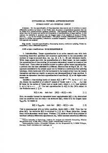
adjacent rows and columns can be removed and much higher compression ratios can be achieved. Second, the resulting basis matrices ��� and ��� in (4) are much smaller than the matrix ����� in [Vasilescu and Terzopoulos 2004], and therefore much less expensive to compute. Third, because there are more basis matrices, each of them does not need to be truncated as much to achieve the same compression ratio. Fig. 6 and 7 compare our tensor representation against PCA and TensorTexture [Vasilescu and Terzopoulos 2004] using the captured BTFs from [Koudelka et al. 2003]. For the convenience of comparison, we actually used 45 views and 60 illumination directions from each BTF, and the image resolution is 192x192. It can be easily verified that processing each color channel separately does not affect tensor approximation results. For each channel, our scheme constructs a 4th-order tensor with size 192x192x45x60; TensorTexture adopts a 3rd-order tensor with size 36864x45x60; PCA organizes the data into a matrix of size 36864x2700. Note that TensorTexture only compresses the view and illumination modes while maintaining the original image resolution. We also did experiments on a
�
��
�
�
2
10 Compression Ratio (in Logrithm)
Figure 5: Comparisons of RMS errors obtained for different compression ratios by PCA (black diamonds), TensorTexture (black squares), modified TensorTexture (blue triangles), and our method (red circles). The top diagram shows the errors for a LICHEN BTF, and the bottom one shows the errors for a VELVET BTF.
ify the reduced ranks (columns) of the four basis matrices for the four modes. The reduced ranks are provided by the user to control the approximation error in (1). The smaller they are, more compact the resulting new tensor is. Given the reduced ranks, the out-of-core tensor approximation algorithm in Section 3.3 is applied to solve for the reduced basis matrices and the core tensor, �� � . The reduced basis matrices and the core tensor together comprise the compact representation. The process of reconstructing a BTF image from our 4th-order tensor is outlined in Figs. 3 and 4. As shown in Fig. 3, if we take one column vector � from ��� and another column vector � from ��� , the tensor between them, � � , defines a basis image. All such basis images together interact with the core tensor, �� � , to produce a different set of basis images, shown in Fig. 4(a), for different view and illumination directions. Mathematically, the second set of basis images are obtained by performing �� � � �� � � ��� � ��� where �� � � ���� ���� �� � �� �� . Then, if we take a pair of row vec� tors, and , from ���� and ���� , respectively, the BTF image associated with the corresponding illumination and view directions can be reconstructed by performing �� � . Fig. 4(b) shows reconstructed BTF images of LEGO. Our tensor representation has clear advantages compared to the one used in [Vasilescu and Terzopoulos 2004]. First, by representing an image as a second-order subtensor, the redundancies between
�
Our Method Modified TensorTexture PCA TensorTexture
10
� ���� � ���� ����� ����� � (4) where ���� � ����� ����� , ���� � ���� ���� , ����� � � �� � , ����� � �� �� �� �� , and �� � � � � ���� ���� �� � �� �� � . ��� � ��� � ���� and ���� spec�
3
10
15
of such directions become much denser, retaining the original two dimensions would likely achieve better compression ratios. To remove redundancy and produce a compact representation, we use another fourth-order tenser ��� � with reduced ranks to approximate �� � as in Section 2.2. The new tensor is represented as: �� �
2
10 Compression Ratio (in Logrithm)
5
�
�
To appear in ACM Transactions on Graphics (Special Issue of SIGGRAPH 2005)
(a) Original
(b) PCA 1.88 RMS Error
(c) TensorTexture 4.21 RMS Error
(d) Our Method 1.87 RMS Error
(e) Modified TensorTexture 2.19 RMS Error
(f) TensorTexture 5.71 RMS Error
(g) Our Method 1.92 RMS Error
Figure 6: A comparison of reconstructed images from PCA, TensorTexture and our tensor representation. The original VELVET BTF has 45 views and 60 illumination directions, and the image resolution is 192x192. A compression ratio of 12, which is equivalent to 91.7% compression, is used for all the methods. (a) Original image. (b) PCA. (c)&(f) TensorTexture. There are 15 views and 15 illums for (c), and 25 views and 9 illums for (f). TensorTexture does not perform spatial compression. (e) Modified TensorTexture with spatial compression. There are 30 views and 30 illums, but the spatial resolution is compressed to 96x96. (d)&(g) Our method. There are 30 views and 30 illums for (d), and 45 views and 20 illums for (g). The spatial resolution is compressed to 96x96 in both.
been successfully applied to the complete BTFs in [Koudelka et al. 2003]. These BTFs have 90 view directions and 120 illumination directions. Our out-of-core algorithm performed significantly better than the PCA-based compression step in [Koudelka et al. 2003]. For the VELVET BTF, the RMS error of the PCA-based compression in [Koudelka et al. 2003] is 4.02 if 150 basis vectors are used while the RMS error of our tensor-based algorithm is only 2.24 if the same compression ratio is achieved. Just as the PCA coefficients can be encoded with JPEG [Koudelka et al. 2003], the coefficients in our core tensor ���� can also be further encoded to boost the compression ratio. However, this encoding step is left as our future work. Fig. 1 shows a synthetic image of a scene with two BTF-mapped objects. The BTFs are represented as compressed tensors.
modified version of TensorTexture, which compresses the spatial resolution as well. The only difference between our scheme and modified TensorTexture is that our scheme considers an image as a 2nd-order subtensor while modified TensorTexture considers an image as a vector. Fig. 5 shows comparisons of RMS errors obtained by the aforementioned methods for different compression ratios. Our method consistently produces the least RMS error in all scenarios. It should be noted that PCA produces comparable results for the VELVET sample at small compression ratios. The RMS errors for our method were obtained using the same reduced ranks for both view and illumination. The results can be further improved if we tune the ranks of these two modes separately. The RMS errors for TensorTexture were obtained by choosing the minimum error among three cases where the rank for view is greater than, equal, or less than the rank for illumination, respectively. The RMS error is actually not a good error metric for the VELVET BTF shown in Fig. 6 since the velvet surface has tiny light-colored dots which tend not to affect RMS significantly. Nevertheless, these dots are preserved surprisingly well by our method. It can be easily verified that the reconstructed images from our tensor representation produces the best results both visually and numerically among the methods we have tested. Visually, our method faithfully preserves high-resolution details during compression. In terms of RMS error, our scheme is the only one that generates an error lower than PCA. The same conclusions hold for all the BTFs we have tested. In the worst case, our result is still slightly better than PCA. In general, as long as there are a relatively large number of image rows and columns and there is redundancy among them, our subtensor representation can achieve a significant improvement because only a small set of basis vectors are necessary to approximate all the rows and columns. We did not use our out-of-core technique (Section 3.3) on these examples because they are sufficiently small. However, this has no bearing on the results obtained as our out-of-core algorithm only manages memory usage and does not affect the quality of tensor approximation. In a separate set of experiments, our out-of-core algorithm has
4.2 Dynamic BTF modeling and compression A conventional BTF describes the appearance of a static surface region while there are many deforming surfaces. We define a dynamic BTF by associating a potentially distinct BTF with any instant in time. Such a dynamic BTF describes the dynamic appearance of a surface with changing geometric or photometric properties. With the additional temporal axis, a dynamic BTF is a seven-dimensional function that demands a compact representation. There has been previous work on rendering deformable objects using a static BTF [Furukawa et al. 2002] or reflectance field [Weyrich et al. 2005]. The basic idea is to resample the static BTF according to the deformation. Our dynamic BTF is different in that the BTFs associated with different times are not simply the warped versions of a static BTF. They are true changing BTFs of the underlying dynamic surface. We organize a dynamic BTF as a fifth-order tensor, ��� � � ���� ���� �� � �� �� ��� � � , using the same notation as in Section 4.1 and ��� � is the number of time samples (frames). By running the out-of-core algorithm in Section 3.3, we can obtain a new tensor ���� � which best approximates ��� � . The new
6
To appear in ACM Transactions on Graphics (Special Issue of SIGGRAPH 2005)
(a) Original
(b) PCA 9.06 RMS Error
(c) TensorTexture 22.56 RMS Error
(d) Our Method 8.22 RMS Error
(e) Modified TensorTexture 10.66 RMS Error
(f) TensorTexture 23.34 RMS Error
(g) Our Method 9.02 RMS Error
Figure 7: A comparison of reconstructed images from PCA, TensorTexture and our tensor representation. The original LEGO BTF has 45 views and 60 illumination directions, and the image resolution is 192x192. A compression ratio of 48, which is equivalent to 97.9% compression, is used for all the methods. (a) Original image. (b) PCA. (c)&(f) TensorTexture. There are 7 views and 8 illums for (c), and 14 views and 4 illums for (f). TensorTexture does not perform spatial compression. (e) Modified TensorTexture with spatial compression. There are 30 views and 30 illums, but the spatial resolution is compressed to 48x48. (d)&(g) Our method. There are 30 views and 30 illums for (d), and 45 views and 20 illums for (g). The spatial resolution is compressed to 48x48 in both.
core algorithm divided each of these huge tensors into 72 blocks and successfully compressed it down to 75x150x28x14x80. It took a 3.4GHz Intel processor with 2GB memory around 60 hours to finish the computation. Once we have this compressed tensor, it takes only 2 seconds to reconstruct an image for the pool given an arbitrary time and an arbitrary pair of view and illumination directions. This performance is achieved by software rendering on the same Intel 3.4GHz processor. It can be potentially improved by GPU-based rendering which is left for future research. Given the compressed tensor with all the information, we can extract interesting subtensors. If we fix the illumination and view directions and vary time, we are simply playing back a conventional fluid animation. If we fix the time only, we obtain a BTF for the water surface at a specific instant. If we fix the view only, we can play back the fluid animation with a simultaneously changing lighting condition. Fig. 8 shows one frame of an animation generated in this way. Complete animations generated from the compressed tensor can be found in the accompanying video. Note that the interpolation scheme for the view and illumination directions [Vasilescu and Terzopoulos 2004] can be applied to time as well. Thus, we can play back different portions of the water motion at different speeds. Animations with varying speeds can also be found in the video.
Figure 8: A water pool mapped with a dynamic BTF in tensor representation. This image shows the appearance of the pool during sunset. tensor is formulated as:
�
��� �
�
� ��� � �
���� ����� ����� ����� ��� �
�
(5) is the reduced rank for
where �� � � ��� � ��� � , and �� � the temporal mode. We have applied our out-of-core tensor approximation to a synthetically generated dynamic BTF which specifies the appearances of the dynamic water surface in a pool. 240 frames of the dynamic water surface were first generated from a computational fluid simulator based on [Enright et al. 2002]. Then for the water surface in each simulated frame, we use a ray tracer to synthetically render a set of BTF images for all combinations of 28 views and 28 illumination directions. The maximum resolution of the image region covering the pool is 180x300. It took nine 2.4GHz PCs more than one week to precompute all the images. The total amount of data is about 30GB. The size of the initial 5th-order tensor for each color channel of this dynamic BTF is 180x300x28x28x240. Our out-of-
4.3 Temporal volume data compression Many computer animation and simulation techniques generate data in a three-dimensional volume grid. The generated volume data is actually four-dimensional with the volume grid accounting for three dimensions and the time being the fourth. The size of such datasets is enormous, and needs compression, especially when a grid resolution is high. Although much work has been performed on compressing static 3D volume data using mathematical tools, such as DCT and wavelet decomposition [Yeo and Liu 1995; Rodler 1999; Nguyen and Saupe 2001], techniques for compressing 4D dynamic volume data as a whole are still under development.
7
To appear in ACM Transactions on Graphics (Special Issue of SIGGRAPH 2005)
(a) Original
(b) 94.4% compression 0.0066 RMS Error
(c) 95.8% compression 0.0083 RMS Error
(d) 97.8% compression 0.014 RMS Error
(e) Origianl
(f) 93.8% compression 0.0681 RMS Error
(g) 95.3% compression 0.0696 RMS Error
(h) 96.9% compression 0.0699 RMS Error
Figure 9: Tensor approximation of volumetric smoke simulations. (a) An original smoke simulation with 480 temporal frames and a volume resolution of 128x128x128. The smoke density values fall between the interval, [0, 1.065]. The spatial resolution is compressed to 64x64x64 in (b)-(d). The temporal resolution is compressed to 200 in (b), 150 in (c) and 80 in (d). Each out-of-core compression divided the original tensor into 32 blocks and took 11.3 hours on a 2.4GHz processor with 784MB RAM. (e) Another smoke simulation with 320 temporal frames and a volume resolution of 100x100x100. The smoke density values fall between the interval, [0, 5.688]. The spatial resolution is compressed to 50x50x50 in (f)-(h). The temporal resolution is compressed to 160 in (f), 120 in (g) and 80 in (h). Each out-of-core compression divided the original tensor into 32 blocks and took 2.2 hours on a 2.4GHz processor with 784MB RAM.
5
We apply tensor-based approximation again to dynamic volume data to obtain a compressed representation. Initially, the original data is organized as a fourth-order tensor, ���� � � ��� ��� ��� � � � , where � , �! and �" represent the grid resolution along each dimension of the volume, and ��� � is the number of simulated frames. To remove redundancy, we use another fourth-order tenser ����� with reduced ranks to approximate ���� as in Section 2.2. The new tensor is represented as:
�
����
where
��� �
�
�
� ���� �
� �
�
� ��� � � , �! � � ��� � , and
�
� �! �
�" ��� � �
� ��� , �
We presented an out-of-core algorithm for higher-order tensor approximation. The basic idea is to partition a tensor into smaller blocks and perform tensor-related operations blockwise. An additional feature of this algorithm is that it effectively exploits the spatial redundancy of multi-dimensional data item to achieve higher compression ratios. With the increasing popularity of data-driven models in graphics, such an out-of-core algorithm becomes indispensable for extracting compact representations. Although we presented three applications here, the promise of this algorithm extends far beyond that. In future, we would like to consider additional applications, such as light fields, complete reflectance fields and other physically simulated data. It is also possible to use this algorithm for data with irregular connectivity, such as meshes, by parameterizing them onto a rectangular domain [Gu et al. 2002]. We would like to explore the prospects of using GPUs to perform tensor reconstruction and multilinear image rendering. We also plan to further design an efficient encoder based on tensor approximation for multi-dimensional datasets. Currently, the reduced ranks of the approximating tensor are specified by the user. It would be helpful if they can be automatically and efficiently found given a desired RMS error threshold.
(6)
�" � ��� ��� , � ��� ��� ��� � .
�
�
����
�
�
Discussions
� ! � " and �� � specify the reduced ranks (columns) of the four basis matrices for the four modes. Without decomposing the three dimensions of a volume using three basis matrices as suggested in Section 3.1, we would have to convert each volume into an extremely long vector, which is infeasible.
We have successfully applied our out-of-core tensor approximation to multiple smoke simulation sequences each of which has between 2.5GB and 10GB of original data. They were originally generated from a controllable smoke simulator in [Shi and Yu 2005]. Our out-of-core algorithm was run on a PC with only 784MB memory. In each simulated frame, there is a 3D smoke density distribution of the uniform volume grid. We store such density distributions on disks using double-precision floating point numbers. They typically have smooth spatial variations and strong temporal coherence, creating much spatial and temporal redundancy. Results for two smoke sequences are shown in Fig. 9 where the images are synthetically rendered using smoke density distributions obtained after tensor-based compression and decompression. These images are quite similar to the images rendered from the original smoke density distributions.
Acknowledgments We wish to thank the authors of [Koudelka et al. 2003] for sharing their BTF database, and the anonymous reviewers for their valuable comments. This work was partially supported by National Science Foundation (CCR-0132970) and Office of Naval Research (N00014-03-1-0107). The first author was supported by UIUC CSE fellowship.
8
To appear in ACM Transactions on Graphics (Special Issue of SIGGRAPH 2005)
References
N GUYEN , K., AND S AUPE , D. 2001. Rapid high quality compression of volume data for visualization. Compuer Graphics Forum 20, 3, 49–56.
B RAND , M. 2002. Incremental singular value decomposition of uncertain data with missing values. In Proc. European Conference on Computer Vision (Vol. I), 707–720.
N ISHINO , K., S ATO, Y., AND I KEUCHI , K. 1999. Eigen-texture method: appearance compression based on 3d model. In Proceedings of IEEE Conference on Computer Vision and Pattern Recognition (CVPR’99), 618–624.
C HEN, W.-C., B OUGUET, J.-Y., C HU , M., AND G RZESZCZUK , R. 2002. Light field mapping: Efficient representation and hardware rendering of surface light fields. ACM Transactions on Graphics 21, 3, 447–456.
R ABANI , E., AND T OLEDO , S. 2001. Out-of-core svd and qr decompositions. In Proceedings of the 10th SIAM Conference on Parallel Processing for Scientific Computing.
DANA , K. J., VAN G INNEKEN , B., NAYAR , S. K., AND KOEN DERINK , J. J. 1999. Reflectance and texture of real world surfaces. ACM Transactions on Graphics 18, 1, 1–34.
RODLER , F. 1999. Wavelet based 3d compression with fast random access for very large volume data. In Proceedings of the 7th Pacific Conference on Computer Graphics and Applications, 108–117.
E NRIGHT, D., M ARSCHNER , S., AND F EDKIW, R. 2002. Animation and rendering of complex water surfaces. ACM Transactions on Graphics 21, 3, 736–744.
S ATTLER , M., S ARLETTE, R., AND K LEIN , R. 2003. Efficient and realistic visualization of cloth. In Proc. Eurographics Symposium on Rendering, 167–177.
F URUKAWA , R., K AWASAKI , H., I KEUCHI , K., AND S AKAUCHI , M. 2002. Appearance based object modeling using texture database: Acquisition, compression, and rendering. In 13th Eurographics Workshop on Rendering, 257–265.
S HASHUA , A., AND L EVIN , A. 2001. Linear image regression and classification using the tensor-rank principle. In IEEE Conf. Computer Vision and Pattern Recognition.
G U , X., G ORTLER , S., AND H OPPE , H. 2002. Geometry images. ACM Transactions on Graphics 21, 3, 355–361.
S HI, L., AND Y U , Y. 2005. Controllable smoke animation with guiding objects. ACM Transactions on Graphics 24, 1, 140–164.
H AN , J., AND P ERLIN , K. 2003. Measuring bidirectional texture reflectance with a kaleidoscope. ACM Transactions on Graphics 22, 3, 741–748.
T ONG, X., Z HANG , J., L IU , L., WANG , X., G UO , B., AND S HUM, H.-Y. 2002. Synthesis of bidirectional texture functions on arbitrary surfaces. In SIGGRAPH 2002 Proceedings, 665–672.
JAMES , D., AND FATAHALIAN , K. 2003. Precomputing interactive dynamic deformable scenes. ACM TOG 22, 3, 879–887. KOUDELKA , M., M AGDA , S., B ELHUMEUR, P., AND K RIEG MAN , D. 2003. Acquisition, compression, and synthesis of bidirectional texture functions. In 3rd Intl. Workshop on Texture Analysis and Synthesis, 59–64.
T UCKER , L. 1966. Some mathematical notes on three-mode factor analysis. Psychometrika 31, 279–311. VASILESCU, M. A. O., AND T ERZOPOULOS , D. 2002. Multilinear analysis of image ensembles: Tensorfaces. In European Conference on Computer Vision, 447–460.
K ROONENBERG , P., AND DE L EEUW, J. 1980. Principal component analysis of three-mode data by means of alternating least squares algorithms. Psychometrika 45, 324–1342.
VASILESCU, M., AND T ERZOPOULOS , D. 2004. Tensortextures: Multilinear image-based rendering. ACM Transactions on Graphics 23, 3, 334–340.
L ATHAUWER , L. D., DE M OOR , B., AND VANDEWALLE , J. 2000. A multilinear singular value decomposition. SIAM J. Matrix Analysis and Applications 21, 4, 1253–1278.
WANG, H., AND A HUJA , N. 2003. Facial expression decomposition. In Int. Conf. on Computer Vision, 958–965.
L ATHAUWER , L. D., DE M OOR , B., AND VANDEWALLE , J. 2000. On the best rank-1 and rank-( � � � � � � ) approximation of higher-order tensors. SIAM J. Matrix Analysis and Applications 21, 4, 1324–1342.
W EYRICH , T., P FISTER , H., AND G ROSS , M. 2005. Rendering deformable surface reflectance fields. IEEE Trans. Visualization and Computer Graphics 11, 1, 48–58.
L EUNG , T., AND M ALIK , J. 1999. Recognizing surfaces using three dimensional textons. In Intl. Conf. Computer Vision.
YANG , J., Z HANG , D., F RANGI, A., AND YANG , J. 2004. Twodimensional pca: A new approach to appearance-based face representation and recognition. IEEE Transactions on Pattern Analysis and Machine Intelligence 26, 1 (January).
L EVOY, M., AND H ANRAHAN , P. 1996. Light field rendering. In Computer Graphics Proceedings, Annual Conference Series, 31–42.
Y E , J. 2004. Generalized low rank approximations of matrices. In International Conference on Machine Learning, ICML’04.
L IU , X., Y U , Y., AND S HUM , H.-Y. 2001. Synthesizing bidirectional texture functions for real-world surfaces. In Proceedings of SIGGRAPH, 97–106.
Y EO, B.-L., AND L IU , B. 1995. Volume rendering of dct-based compressed 3d scalar data. IEEE Trans. Visualization and Computer Graphics 1, 1, 29–43.
L IU , X., H U , Y., Z HANG , J., T ONG, X., G UO , B., AND S HUM , H.-Y. 2004. Synthesis and rendering of bidirectional texture functions on arbitrary surfaces. IEEE Trans. Visualization and Computer Graphics 10, 3, 278–289.
Y U , Y., AND C HANG , J. 2005. Shadow graphs and 3d texture reconstruction. International Journal of Computer Vision 62, 1/2, 35–60.
M ATUSIK , W., P FISTER , H., B RAND , M., AND M C M ILLAN , L. 2003. A data-driven reflectance model. ACM Transactions on Graphics 22, 3, 759–769.
9