Geophysical Research Letters RESEARCH LETTER 10.1002/2015GL065140 Key Points: • Inefficient cloud overlap at small scales is now supported by observations • Inverse linear functions best describe cloud overlap • LES and observations both indicate a diurnal cycle in the overlap parameter
Supporting Information: • Figure S1
Correspondence to: E. Orlandi,
[email protected]
Citation: Corbetta, G., E. Orlandi, T. Heus, R. Neggers, and S. Crewell (2015), Overlap statistics of shallow boundary layer clouds: Comparing ground-based observations with large-eddy simulations, Geophys. Res. Lett., 42, 8185–8191, doi:10.1002/2015GL065140.
Received 6 JUL 2015 Accepted 17 AUG 2015 Accepted article online 21 AUG 2015 Published online 8 OCT 2015 Corrected 3 DEC 2015
This article was corrected on 3 DEC 2015. See the end of the full text for details.
©2015. The Authors. This is an open access article under the terms of the Creative Commons Attribution-NonCommercial-NoDerivs License, which permits use and distribution in any medium, provided the original work is properly cited, the use is non-commercial and no modifications or adaptations are made.
CORBETTA ET AL.
Overlap statistics of shallow boundary layer clouds: Comparing ground-based observations with large-eddy simulations G. Corbetta1 , E. Orlandi1 , T. Heus1,2 , R. Neggers1 , and S. Crewell1 1 Institute for Geophysics and Meteorology, University of Cologne, Cologne, Germany, 2 Now at Department of Physics,
Cleveland State University, Cleveland, Ohio, USA
Abstract High-resolution ground-based measurements are used to assess the realism of fine-scale numerical simulations of shallow cumulus cloud fields. The overlap statistics of cumuli as produced by large-eddy simulations (LES) are confronted with Cloudnet data sets at the Jülich Observatory for Cloud Evolution. The Cloudnet pixel is small enough to detect cumuliform cloud overlap. Cloud fraction masks are derived for five different cases, using gridded time-height data sets at various temporal and vertical resolutions. The overlap ratio (R), i.e., the ratio between cloud fraction by volume and by area, is studied as a function of the vertical resolution. Good agreement is found between R derived from observations and simulations. An inverse linear function is found to best describe the observed overlap behavior, confirming previous LES results. Simulated and observed decorrelation lengths are smaller (∼300 m) than previously reported (> 1 km). A similar diurnal variation in the overlap efficiency is found in observations and simulations.
1. Introduction As large-scale models for weather and climate have coarse spatial resolutions, they cannot resolve clouds within a vertical grid column and thus rely on parameterizations, leading to uncertainty in the representation of clouds and the way they overlap in the vertical. Even though cloud overlap is somewhat balanced out by inhomogeneous distributions of ice and liquid inside the clouds, the uncertainty in the cloud overlap parameterization remains a significant source of error in the Earth’s radiation budget in general circulation models (GCMs) [Shonk and Hogan, 2010] which is the reason why cloud overlap has been widely researched. Most studies concerning cloud overlap mainly focused on either the whole troposphere [e.g., Hogan and Illingworth, 2000] or deep convective cloud fields [e.g., Pincus et al., 2005], while cumuliform boundary layer cloud fields have been less researched because of their irregularity in shape and in spatial distribution at subgrid scales. Brown [1999] and Brooks et al. [2004] did report poor vertical overlap of shallow boundary layer cumuli using large-eddy simulations (LES) and ground-based measurements respectively, but these studies did not further investigate its dependence on layer depth. Neggers et al. [2011] provided a more detailed analysis of overlap behavior based on three case studies simulated by the Dutch Atmospheric LES (DALES) model [Heus et al., 2010]. They distinguish between “supergrid-scale” overlap, i.e., the vertical overlap of cloud fraction between grid boxes in a GCM column, and “subgrid-scale” overlap, representing the irregularity and spatial distribution at vertical scales smaller than the GCM grid box. In their study, the overlap ratio R = Cv ∕Ca (see Del Genio et al. [1996] and Brooks et al. [2004] for the definition of cloud cover by area Ca and by volume Cv ) was used to express overlap efficiency, with high (low) R values reflecting efficient (inefficient) vertical overlap between cloud elements at different heights. Its dependence on sampling layer thickness, to be interpreted as a model level thickness in a GCM, was investigated, and an inverse linear functional form was found to best reproduce the LES results. This study aims to seek observational support for the numerical results of Neggers et al. [2011], making use of high-resolution ground-based observations at the Jülich Observatory for Cloud Evolution (JOYCE). To this purpose, five appropriate cloud cases during the April–August 2013 period are selected for investigation, representing a variety of shallow cumulus-topped boundary layers. For the first time, cloud overlap statistics will be derived from both measurements and accompanying realistic LES, allowing their direct comparison. CLOUD OVERLAP STATISTICS
8185
Geophysical Research Letters
10.1002/2015GL065140
Figure 1. Time-height section of Cloudnet cloud classification on 27 April 2013 with inlet illustrating a model grid with 15 min temporal and 1500 m vertical resolution. Ice pixels are yellow; liquid pixels are light blue.
2. Observational Method and Data 2.1. Observations The measurements used in this study were performed at the Jülich Observatory for Cloud Evolution (JOYCE) [Löhnert et al., 2014], including cloud radar, ceilometer, and microwave radiometer. Five case studies in April–August 2013 are selected, and the Cloudnet classification algorithm of Illingworth et al. [2007] is applied to distinguish clear sky from cloudy pixels and to further separate liquid from ice phase. Pixel size is defined by cloud radar temporal (30 s) and range resolution (30 m). In order to mimic the typical discretization of large-scale models, daily time-height sections of the cloud masks are divided into equally sized grid boxes, using a temporal resolution of 3 or 15 min (which, assuming the mean advective wind speed to be 10 m/s, correspond, respectively, to 2 and 9 km) and a vertical discretization ranging from 60 to 1500 m. The coarsest time resolution (15 min) was not used for two (27 April and 19 May) of the five days under examination due to the employed radar scanning strategy, which included 3 min of off-zenith measurements every 6 min (see Figure 1). For each grid box, Ca and Cv are computed, which allows calculation of the overlap ratio. Clear-sky (i.e., Ca = Cv = 0) and full-cloudy (i.e., Ca = Cv = 1) grid boxes are ruled out from the computation. Means of the overlap ratio over the period of the day featuring boundary layer clouds (referred in the following text as daily mean) or over 1 h (hourly mean) can then be studied as a function of layer depth. For reference cloud overlap will also be expressed in terms of the decorrelation length as proposed by Hogan and Illingworth [2000]. 2.2. DALES Simulations Large-eddy simulations are performed for the same cases, making use of the DALES code and adopting the model configuration as described by Neggers et al. [2012]. In this setup, the LES is homogeneously driven by time-dependent large-scale forcings derived from analysis data. In this study analysis, data from the operational numerical weather prediction system Integrated Forecasting System of the European Centre for Medium-Range Weather Forecasts (ECMWF) is used. Smaller-scale processes, unresolved by the forecast model, including turbulence, radiation, cumulus cloud physics, and dynamics, are explicitly calculated (i.e., resolved) by the LES model, which can thus be interpreted as a local downscaling of the GCM larger-scale state. The DALES code also includes a land surface parametrization, which closely resembles the ECMWF parametrization (see Heus et al. [2010], for more details). The simulations are performed on a domain of 12.8 × 12.8 × 5 km, at a resolution of 50 m in the horizontal directions and 40 m in the vertical direction. Every simulation covers one diurnal cycle, starting at midnight. Only the daytime period of the simulations is considered; the hours before sunrise are regarded as spin-up and not included in any analysis. The overlap ratio in the LES simulations could be computed straightforwardly as the ratio of domain-mean values of Cv and Ca , but this would not be consistent with the observations. Instead, the overlap ratio in LES is calculated from single columns sampled from the three-dimensional grid at fixed locations at a frequency of 1∕30 s−1 , using the identical procedure as applied in the processing of the observational data.
3. Results 3.1. Overlap Ratio in Shallow Cumuli Figure 2a shows the daily mean overlap ratio as a function of layer depth (15 min time resolution) for the 5 June 2013, which featured a clear-sky day, with shallow boundary layer clouds developing in the early afternoon CORBETTA ET AL.
CLOUD OVERLAP STATISTICS
8186
Geophysical Research Letters
10.1002/2015GL065140
(a)
(b)
Figure 2. Overlap ratio R as a function of vertical grid resolution h on 5 June 2013: (a) daily mean values (diamonds) and inverse linear fitting curves (thick lines) from model and observations and (b) hourly mean values (diamonds) and inverse linear fitting curves (thick lines) between 10:30 UTC and 15:30 UTC from observations only. Error bars are the standard deviation of the mean overlap ratio within the time period considered. LES simulations have been forced using ECMWF analysis.
(base height ranging from 1 to 2 km). Observed and DALES-simulated overlap ratios were least squares fitted using the inverse linear functional form R = (1 + 𝛽h)−1
(1)
with h being the layer depth. The fit parameter is found to be 𝛽 = 6.3 × 10⁻³ m−1 when derived from the DALES simulation, compared with 𝛽 = 5.2 × 10⁻³ m−1 for observations. These values are roughly similar to those reported by Neggers et al. [2011] for LES of subtropical marine shallow cumulus and thus corroborates with their numerical results on cumuliform cloud overlap inefficiency. Alternatively, the projected cloud cover Cp can be expressed as a blend between the limit cases of maximum (Cmax ) and random (Crand ) overlap: Cp = 𝛼Cmax + (1 − 𝛼)Crand
(2)
with blending parameter 𝛼 as a function of the layer thickness Δz: ( ) Δz 𝛼 = exp − Δz0
(3)
in which Δz0 is the decorrelation length. Table 1 lists the 𝛽 values for all five selected cases, calculated using daily mean values of R, at both 3 and 15 min time resolutions. The associated decorrelation length [Hogan and Illingworth, 2000], fitted over the first 200 m, is also given for reference. Good agreement between observations and LES is reported for all cases and at both time resolutions, suggesting that overlap in the model clouds is similar to that observed in nature. Note that the decorrelation lengths are all much smaller (mostly less than 300 m) than previously Table 1. 𝛽 Parameter (m−1 ) (Fitted Using Daily Mean R Values) and Decorrelation Length (m) on Different Days in 2013 Featuring Boundary Layer Clouds Calculated From Observations and LES Simulations for 3 and 15 min Time Resolutions 3 min 𝛽 × 103
Day
CORBETTA ET AL.
15 min
Decorrelation Length
𝛽 × 103
Decorrelation Length
Observations
LES
Observations
LES
Observations
LES
Observations
LES
27 Apr
4.9
4.5
590
180
-
-
-
-
19 May
5.8
6.2
157
127
-
-
-
-
5 Jun
4.7
6.5
160
148
5.2
6.3
170
202
10 Jun
4.4
4.9
253
104
4.7
5.7
213
153
20 Aug
5.3
6.6
249
120
5.0
7.0
237
239
CLOUD OVERLAP STATISTICS
8187
Geophysical Research Letters
10.1002/2015GL065140
Table 2. Comparison of 𝜒 2 Values on Different Days in 2013 Featuring Boundary Layer Clouds Derived From Fitting Inverse Linear and Power Law Functions to Overlap Ratio Versus Layer Depth, Using Observational Data at 3 and 15 min Time Resolutions 3 min Day 27 Apr
15 min
Inverse Linear
Exp.
Inverse Linear
Exp.
2.0
3.6
-
-
19 May
2.1
3.1
-
-
5 Jun
3.2
8.4
1.2
3.6
10 Jun
12.2
16.6
7.0
8.0
20 Aug
4.4
10.3
2.7
5.0
reported values (> 1 km), even those derived from cloud-resolving model simulations [e.g., Oreopoulos and Khairoutdinov, 2003; Pincus et al., 2005]. This supports the general conclusion by Neggers et al. [2011] that overlap in cumuliform clouds, when detected at small scales, is much more random, or inefficient, compared to other cloud types. It is tempting to interpret the relatively large 𝛽 values, reflecting that the overlap ratio drops quicker with increasing layer depth, as typical for boundary layer shallow cumuli. To further investigate the validity of this assumption, the overlap is calculated for the whole troposphere for the 27 April 2013, which featured an elevated and thick stratiform ice cloud layer between 4 and 7 km height (see also Figure 1). For this cloud scene the observed fit yielded a value 1 order of magnitude smaller (𝛽 = 6 ×10⁻⁴ m−1 ), suggesting a much more efficient overlap when high-altitude large-scale clouds are included. This emphasizes that different cloud types are associated with very different overlap behavior. A further relation between Ca and Cv proposed in literature [Brooks et al., 2004] is given in equation (4): Ca = [1 + exp(−f ) ⋅ (Cv−1 − 1)]−1
(4)
with f as a fit parameter. Figures S1a and S1b in the supporting information show the scatterplots of Ca versus Cv at 15 min averaging time, together with the fitted curves using equation (4), for three different vertical resolutions. As expected for the low cloud cover that is typical for shallow boundary layer cumuli, our data set fills the lower left corner of Figure 7 in Brooks et al. [2004], showing both small Cv and Ca values. In this limit, (4) reduces to Ca = ef Cv so that our R = e−f . The comparison between Figures S1a and S1b shows that Cv and Ca cluster in the same region when calculated using LES and observations, even though the LES Cv , Ca couples exhibit a larger dynamic range. Figure S1c shows a very good agreement between LES and observations regarding the dependency of f as a function of the layer depth h. There is also a good qualitative agreement between Figure S1c and the dependency of f on vertical resolution shown in Figure 9 of Brooks et al. [2004] for horizontal grid separation smaller than 10 km. 3.2. Numerical Fitting of Overlap Ratio In the previous section an inverse linear form was selected to least squares fit the data, a choice motivated by (i) results of previous studies and (ii) the convenience of having the overlap efficiency expressed by a single constant of proportionality (𝛽 ). However, other functional forms can be thought of to represent the relationship between R and the vertical grid box dimension h. Three candidate functional relationships were tested by Neggers et al. [2011] using large-eddy simulations of three different cumulus cases, asking which one best describes the overlap ratio as a function of layer depth. They reported that the inverse linear fit had the lowest root-mean-square error compared to the exponential and power law fits. We repeated this exercise by least squares fitting our observed data for five different case studies with various candidate functions, including the inverse linear function equation (1), a power law equation (5), and the exponential form equation (6): R = ahb
(5)
R = exp(−h∕H).
(6)
The associated chi-square values were then compared. For 5 June 2013, at 15 min temporal resolution, the chi-square value associated with the inverse linear fit is lower (𝜒 2 = 1.2, 𝛽 = 5.2×10⁻³ m−1 ) than that resulting from the power law fit (𝜒 2 = 3.6, a = 5.5, b = −0.45) and from the exponential (𝜒 2 = 20, H = 390 m). Table 2 CORBETTA ET AL.
CLOUD OVERLAP STATISTICS
8188
Geophysical Research Letters
10.1002/2015GL065140
shows the repetition of this exercise for all five cases: the exponential form does not appear as its associated 𝜒 2 value is significantly higher than that for the other two functional forms on all five days. The inverse linear fit proved to be systematically more accurate than the power law fit, and this is independent of temporal resolution, thus confirming what was suggested by Neggers et al. [2011]. 3.3. Diurnal Cycle of 𝜷 The inverse linear fit can be used to investigate the time evolution of 𝛽 during the diurnal development of the shallow cumulus-capped boundary layer. To this −1 Figure 3. Time series of fit parameter 𝛽 (m ) on the 5 June 2013 from purpose we focus on 5 June 2013, choobservations (black) and ECMWF-driven (blue) LES simulation for two sen here because this case closely randomly chosen locations. Error bars are standard error of mean 𝛽 parameter over the time period under examination. resembles the prototype view of a transient cumulus-topped boundary layer over land. The time period between 10:30 UTC and 15:30 UTC, when cumuli were present, is discretized into 1 h bins, for each of which the overlap ratio values are averaged using a temporal resolution of 15 min. The inverse linear fit is then applied yielding a 𝛽 value for each subperiod. The hourly mean overlap ratios as a function of h are plotted in Figure 2b, suggesting that the overlap efficiency decreases with diurnal time after cloud onset, with 𝛽 ranging from a minimum at cloud onset (2.2 × 10⁻³ m−1 ) toward a maximum in the 13:30–14:30 UTC period (7.9 × 10⁻³ m−1 ). Figure 3 not only shows the associated observed time series of 𝛽 but also includes LES results at two different random locations in the domain. Interestingly, the DALES runs show a similar pattern, with a progression from minimum 𝛽 values (i.e., more efficient overlap) at cloud onset toward peak values (i.e., less efficient overlap) at a later stage. The question is what controls the observed time development of overlap efficiency. Interestingly, Neggers et al. [2011] reported the opposite trend during another case of transient continental cumulus at the Southern Great Plains site of the Atmospheric Radiation Measurement Program, with overlap becoming more efficient during the day. This is in line with the idea that convection gains strength as the day progresses, perhaps favoring more maximum overlap. For this reason cloud cover has been suggested as a controlling factor [Brooks et al., 2004], as it typically decreases during the day. However, the observations for the 5 June 2013 case presented here do not follow this theory; cloud fraction also decreases, but overlap efficiency decreases. Ongoing research (not shown here) suggests that the size statistics of the cloud population play an important role, finding good correlations between overlap efficiency and maximum cloud size.
Figure 4. Scatterplots of simulated and observed 𝛽 values (m−1 ) for (left) 15 and (right) 3 min time resolutions, calculated using hourly mean values of R.
CORBETTA ET AL.
CLOUD OVERLAP STATISTICS
8189
Geophysical Research Letters
10.1002/2015GL065140
To further assess the realism of the model results, the modeled 𝛽 values based on hourly means for all five cases are plotted against their observed equivalents in Figure 4. Including the diurnal variation broadens the parameter space, which should facilitate any effort at correlation; to further optimize the statistical significance of the comparison, each observed value is plotted against model results sampled at two independent columns in the model domain, 6.4 km apart. This is done at both 3 and 15 min time resolutions. In line with the daily mean results (see Table 1) the LES results are slightly positively biased by 9 × 10⁻⁴ and 5.5 × 10⁻⁴ m−1 for 3 and 15 min time resolutions, respectively, corresponding to 17 and 10% of the observed 𝛽 averaged over all five cases at the corresponding time resolution. Increasing the time resolution from 3 to 15 min does not strongly affect the bias but improves the correlation from 0.2 to 0.5, perhaps due to the associated increased spread in values. Note that while there is no perfect match between the observations and the LES results, the agreement is much better than the order of magnitude difference that results from including multiple cloud forms together, such as the 27 April scene if the ice clouds are included.
4. Discussion and Conclusions Ground-based observations of clouds were used to obtain insight into overlap behavior in cumuliform shallow boundary layer cloud fields and to critically evaluate findings from previous LES analyses. Cumuliform overlap is found to be inefficient when considering only liquid-phase shallow cumuli, due to their irregular shape and spatial distribution at small scales that remain unresolved in GCMs. The research supports the LES results of Neggers et al. [2011], which gives confidence in the skill of the LES approach in realistically simulating natural cumulus clouds, and thus promotes its use as a virtual laboratory for parametrization development for weather and climate models. We find quantitative agreement between LES and observation using three different descriptions of the overlap efficiency, namely, the overlap ratio used in Neggers et al. [2011], the decorrelation length used in Hogan and Illingworth [2000], and the f parameter used in Brooks et al. [2004]. Disagreement with other observational studies, such as Hogan and Illingworth [2000] or Willen et al. [2005], is likely to be related to differences in cloud type and discretization. For example, stratiform ice clouds exhibit highly efficient overlap, so previous studies at midlatitudes covering the whole troposphere and applying coarser discretizations than the ones applied here are therefore weighted toward more efficient overlap. Acknowledgments This research has been jointly financed by the Federal Ministry of Education and Research (BMBF) within the programme High Definition Clouds and Precipitation for advancing Climate Prediction (HD(CP)2) under grant HD(CP)2 01LK1209A and ITARS (www.itars.net), European Union Seventh Framework Programme FP7: People, and ITN Marie Sklodowska Curie Actions Programme under grant agreement 289923. We acknowledge the ECMWF for providing access to the data used to drive the DALES simulations. We acknowledge the Cloudnet project (European Union contract EVK2-2000-00611) for providing the Cloudnet classification, which was produced by the Institute for Geophysics and Meteorology, University of Cologne, using measurements from the JOYCE facilities. LES and Cloudnet data used for this study are available upon request to the authors; the DALES model can be freely downloaded from the website https://github.com/dalesteam/dales. We are grateful to the two anonymous reviewers for their careful reading of the manuscript and constructive comments. The Editor thanks two anonymous reviewers for their assistance in evaluating this paper.
CORBETTA ET AL.
Our research confirms that the inverse linear functional form best describes the dependence of cumuliform overlap efficiency on layer depth. The diurnal cycle of the associated fitting parameter is investigated for a prototype case of shallow cumulus convection, revealing good agreement between the observations and the fine-scale cloud-resolving simulations. The difference in the diurnal time development of overlap efficiency between the case studied here and the case studied by Neggers et al. [2011] is not explained by our research; we speculate that cloud population statistics are at the heart of this discrepancy. Accordingly, while this study answers some key questions concerning cumuliform overlap, it also raises some new questions. We see this study as a first step toward a rigorous verification of LES results, involving continuous long-term LES downscaling at fixed meteorological supersites, where instrumentation is operated continuously that is capable of observing clouds at cumulus-resolving resolutions. Our findings are relevant for studies of climate change, in which clouds play an essential role. The inefficient overlap we found at subgrid vertical scales has the potential of significantly affecting the vertical transfer of radiation [Neggers et al., 2011], yet few GCMs take such overlap at small, unresolved scales into account—rather, volume and area cloud fraction are usually assumed identical. A better understanding of the unresolved cloud overlap now opens the door for parametrizations, where cloud overlap and also in-cloud inhomogeneities are better grounded in physics. Hopefully, this should lead to a more reliable cloud radiative budget in large-scale models.
References Brooks, M. E., R. J. Hogan, and A. J. Illingworth (2004), Parameterizing the difference in cloud fraction defined by area and volume as observed with radar and lidar, J. Atmos. Sci., 62, 2248–2260. Brown, A. R. (1999), Large-eddy simulation and parameterization of the effects of shear on shallow cumulus convection, Boundary Layer Meteorol., 91, 65–80. Del Genio, A. D., M. -S. Yao, W. Kovari, and K. K. Lo (1996), A prognostic cloud water parameterization for global climate models, J. Clim., 9, 270–304. Heus, T., et al. (2010), Formulation of the Dutch Atmospheric Large-Eddy Simulation (DALES) and overview of its applications, Geosci. Model Dev., 3, 415–444, doi:10.5194/gmd-3-415-2010. Hogan, R. J., and A. J. Illingworth (2000), Deriving cloud overlap statistics from radar, Q. J. R. Meteorol. Soc., 126, 2903–2909, doi:10.1002/qj.49712656914.
CLOUD OVERLAP STATISTICS
8190
Geophysical Research Letters
10.1002/2015GL065140
Illingworth, A. J., et al. (2007), Cloudnet—Continuous evaluation of cloud profiles in seven operational models using ground-based observations, Bull. Am. Meteorol. Soc., 88, 883–898. Kato, S., S. Sun-Mack, W. F. Miller, F. G. Rose, Y. Chen, P. Minnis, and B. A. Wielicki (2010), Relationships among cloud occurrence frequency, overlap, and effective thickness derived from CALIPSO and CloudSat merged cloud vertical profiles, J. Geophys. Res., 115, D00H28, doi:10.1029/2009JD012277. Löhnert, U., et al. (2014), JOYCE: Jülich Observatory for Cloud Evolution, Bull. Am. Meteorol. Soc., 96, 1157–1174, doi:10.1175/BAMS-D-14-00105.1. Neggers, R. A. J., T. Heus, and A. P. Siebesma (2011), Overlap statistics of cumuliform boundary-layer cloud fields in large-eddy simulations, J. Geophys. Res., 116, D21202, doi:10.1029/2011JD015650. Neggers, R. A. J., A. P. Siebesma, and T. Heus (2012), Continuous single-column model evaluation at a permanent meteorological supersite, Bull. Am. Meteorol. Soc., 93, 1389–1400, doi:10.1175/BAMS-D-11-00162.1. Oreopoulos, L., and M. Khairoutdinov (2003), Overlap properties of clouds generated by a cloud resolving model, J. Geophys. Res., 108(D15), 4479, doi:10.1029/2002JD003329. Pincus, R., C. Hannay, S. A. Klein, K. M. Xu, and R. Hemler (2005), Overlap assumptions for assumed probability distribution function cloud schemes in large-scale models, J. Geophys. Res., 110, D15S09, doi:10.1029/2004JD005100. Shonk, J. K. P., and R. J. Hogan (2010), Effect of improving representation of horizontal and vertical cloud structure on the Earth’s global radiation budget. Part II: The global effects, Q. J. R. Meteorol. Soc., 116, 1205–1215. Willen, U., S. Crewell, H. K. Baltink, and O. Sievers (2005), Assessing model-predicted vertical cloud structure and cloud overlap with radar and lidar ceilometer observations for the Baltex Bridge Campaign of CLIWA-NET, Atmos. Res., 75(75), 227–255.
Erratum In the originally published version of this article, figure 3 was incorrectly typset. The figure has since been corrected and this version of record.
CORBETTA ET AL.
CLOUD OVERLAP STATISTICS
8191