overloading, subtyping and late binding: functional

´ PARIS 7 Universite

OVERLOADING, SUBTYPING AND LATE BINDING: FUNCTIONAL FOUNDATION OF OBJECT-ORIENTED PROGRAMMING PhD dissertation

January 1994

Advisor: Giuseppe Longo Referees: Kim Bruce Luca Cardelli Didier Rémy Chairperson: Guy Cousineau Committee Members: Serge Abiteboul Jean-Pierre Jouannaud Giuseppe Longo Didier Rémy Patrick Sallé

Giuseppe Castagna Laboratoire d’Informatique de l’Ecole Normale Supérieure

´ PARIS 7 Universite

SURCHARGE, SOUS-TYPAGE ET LIAISON TARDIVE : FONDEMENTS FONCTIONNELS DE LA PROGRAMMATION ´ OBJETS ORIENTEE The`se de doctorat

janvier 1994

Directeur de th` ese : Giuseppe Longo Rapporteurs : Kim Bruce Luca Cardelli Didier Rémy Pr´ esident du Jury: Guy Cousineau Examinateurs : Serge Abiteboul Jean-Pierre Jouannaud Giuseppe Longo Didier Rémy Patrick Sallé

Giuseppe Castagna Laboratoire d’Informatique de l’Ecole Normale Supérieure

Quest tesi è dedicata a mio nonno ’Gin che mi mostr´ o la dolcezza, la bont´ a e la tolleranza, mio nonno Beppe che mi mostr´ o la coerenza e la perseveranza Ilaria e \ldots per i momenti felici passati assieme

Acknowledgments Giuseppe Longo really deserves the first position in this list. It is not the task of a simple PhD. student to praise the scientific qualities of Prof. Longo; but since I had the chance to work with him and to share some of his time, I can witness of his exceptional human qualities. He was always ready to listen to me, to help me in the difficult moments, to calm down with patience my enthusiasms when they were too strong and to tolerate my faults. His attitude was the one of a permanent “learner”: he listens to you to learn from you. Thus I want to thank more the man than the scholar, because if it is true that I owe much to the latter, I am indebted for a more important example to the former. And I am happy to express here all my appreciation for him. All my thanks also to Giorgio Ghelli. This thesis owes him a lot: the incipient intuition, some ideas and results presented in this thesis come from him. The “anschauung” he transmitted me was very helpful to perceive the general setting behind every particular result. Benli Pierce is a great researcher and a friend; thanks to him this thesis has one chapter written in real english (apart from the modifications I made) Luca Cardelli deserves a triple acknowledgment: for having started the type theoretic research on object-oriented programming, for his suggestions and the various discussions I had with him —thanks to him the chapter 8 of this thesis exists—, and for the incredible courage demonstrated in accepting to be the referee of this thesis. The same holds for Kim Bruce, which has my gratitude also for his advice and for the warm hospitality he and his wife Fatima offered me in Williamstown. Didier Rémy completes the list of the audacious who accepted the challenge of judging my thesis; I thank him for this and for the interest he always demonstrated in my work. Thanks a lot to Guy Cousineau, for his help, his amiability and his always ready advice: ´ I owe him a lot. With him I also want to thank the Laboratoire d’Informatique de l’Ecole Normale Supérieure, who offered me a pleasant and stimulating place to develop this work. The other department I want warmly to thank is the DISI of University of Genoa, in the person of Eugenio Moggi: his advice and his comprehension helped me a lot and I really regretted to be obliged to abandon Genoa to end this thesis. Thanks also to the University of Pisa for all the years I spent there and the Consiglio Nazionale delle Ricerche, Comitato Nazionale per le Scienze Matematiche for its financial support. I am also grateful to Mart´ın Abadi whose suggestions the results of section 8.5 come from; to Véronique Benzaken who introduced me to O2 ; to John Lamping who suggested me the study of one of the systems in chapter 4; to John Mitchell for his advice and his hospitality

3

4

at Stanford; to Hideki Tsuiki who pointed me out an error in the semantics for λ&; to Allyn Dimock, Maribel Fernández, and some anonymous referees (I will never say which ones!) for their comments on the drafts of some papers; to Dinesh Katiyar for his courage in assisting four times to the same talk I gave in different places; to Kathleen Milsted for her help in writing the introduction of this thesis; to Bob Muller and his wife Susan for their hospitality during my visit to the Apple-Eastern Research and Technology Lab. and also to the Dylan group for the many stimulating discussions; to Maria Virginia Apónte, Fran¸cois Bouladoux, Lucky Chillan, Pierre Cregut, Adriana Compagnoni, Pierre-Louis Curien, Roberto Di Cosmo, Furio Honsell, Delia Kesner, Simone Martini, Chet Murthy, Pino Rosolini for the discussions I had with them. I also want to thank the friends of these years that are not cited above: Alejandro, Alessandra, Antonio, Carola, Cristina (J. P.-A.), Ilaria, Inés, José, Kiki, Liliane, Mario, Michel, Nadine, Pompeo, Roberto, Tiziana, Tomás(!), Yiyo just because they were there . . . which means a lot. Let me end with the persons who are the demiurges of this thesis: Franca and Nico, my parents. I want to thank them for their constant support; for having trusted in me; for having taught me to take my responsibilities and to respect every other person; for the example they were for me ... in a word: for their love. And if this thesis cannot certainly recompense all they gave to me, could be a comfort to our separation to know that I do love them.

Preface E poi che la sua mano alla mia pose con lieto volto, ond’io mi confortai, mi mise dentro alle segrete cose. Dante Alighieri Inferno; iii, 19-21

Many of the results in this thesis have already been published in review or conference proceedings. More precisely chapters 2 and 3 are based on an article to appear in Information and Computation [CGL92b] whose extended abstract can be found in the proceedings of the 1992 ACM Conference on LISP and Functional Programming [CGL92a]. The first and the fifth chapters are partially based on a paper whose (very) preliminary version appeared as a Technical Report of LIENS [Cas92], and whose extended abstract has been published in the 13th Conference on Foundation of Software Technology and Theoretical Computer Science [Cas93b]. The extended abstract of the sixth chapter appears in the proceedings of the International Conference on Typed Lambda Calculi and Applications [CGL93]. Chapter 9 and part of chapter 10 are contained in a paper actually under submission, whose extended abstract appears in the proceedings of the 4th International Workshop on Data Base Programming Languages [Cas93a]. The extended abstract of chapter 8 will be presented at the 21st Annual Symposium on Principle Of Programming Languages. Finally for the second and the seventh chapter we also used part of the course notes for a summer school in Nice [CL91b]. Most of these papers are coauthored: without the essential contributions of Giorgio Ghelli, Giuseppe Longo and Benjamin Pierce this thesis certainly could not be but much poorer than what it is. We will recall the other authors at the beginning of each chapter whose results are not due only to this thesis’s author.

5

6

Contents Pr´ esentation de la th` ese Programmation orientée objets . . . . . . . . . . . . . . . . . Le λ&-calcul . . . . . . . . . . . . . . . . . . . . . . . . . . . Normalisation Forte . . . . . . . . . . . . . . . . . . . . . . . Trois variations sur le thème . . . . . . . . . . . . . . . . . . Un méta-langage de λ& . . . . . . . . . . . . . . . . . . . . . Sémantique . . . . . . . . . . . . . . . . . . . . . . . . . . . . Second ordre . . . . . . . . . . . . . . . . . . . . . . . . . . . Vers une quantification bornée décidable . . . . . . . . . . . . Quantification bornée avec surcharge . . . . . . . . . . . . . Surcharge de second ordre et programmation orientée objets . Conclusion . . . . . . . . . . . . . . . . . . . . . . . . . . . .

. . . . . . . . . . .

. . . . . . . . . . .

. . . . . . . . . . .

. . . . . . . . . . .

. . . . . . . . . . .

. . . . . . . . . . .

. . . . . . . . . . .

. . . . . . . . . . .

. . . . . . . . . . .

. . . . . . . . . . .

. . . . . . . . . . .

. . . . . . . . . . .

13 18 19 26 27 31 34 37 38 42 45 48

Introduction

53

Background and notation Term rewriting systems . . . . . . . . . . . . . . . . . . . . . . . . . . . . . . . . . Logic . . . . . . . . . . . . . . . . . . . . . . . . . . . . . . . . . . . . . . . . . . . .

61 61 62

I

63

Simple typing

1 Object-oriented programming 1.1 A kernel functional object-oriented language 1.1.1 Objects . . . . . . . . . . . . . . . . 1.1.2 Messages . . . . . . . . . . . . . . . 1.1.3 Methods and functions . . . . . . . . 1.1.4 Classes . . . . . . . . . . . . . . . . 1.1.5 Inheritance . . . . . . . . . . . . . . 1.1.6 Multiple inheritance . . . . . . . . . 1.1.7 Extending classes . . . . . . . . . . . 1.1.8 Super, self and the use of coercions . 1.1.9 Multiple dispatch . . . . . . . . . . . 1.1.10 Messages as first-class values: adding

7

. . . . . . . . . . . . . . . . . . . . . . . . . . . . . . . . . . . . . . . . . . . . . . . . . . . . . . . . . . . . . . . . . . . . . . overloading

. . . . . . . . . . .

. . . . . . . . . . .

. . . . . . . . . . .

. . . . . . . . . . .

. . . . . . . . . . .

. . . . . . . . . . .

. . . . . . . . . . .

. . . . . . . . . . .

. . . . . . . . . . .

. . . . . . . . . . .

. . . . . . . . . . .

. . . . . . . . . . .

65 65 65 66 66 68 70 72 74 75 76 77

8

CONTENTS

1.2

Type checking . . . . . . . . . . . . . . . . . . . . . . . . . . . . . . . . . . . . 1.2.1 The types . . . . . . . . . . . . . . . . . . . . . . . . . . . . . . . . . . 1.2.2 Intuitive typing rules . . . . . . . . . . . . . . . . . . . . . . . . . . . .

2 The λ&-calculus 2.1 Informal presentation . . . . . . . . . . . . . . . . 2.1.1 Subtyping, run-time types and late binding 2.2 The syntax of the λ&-calculus . . . . . . . . . . . . 2.2.1 Subtyping rules. . . . . . . . . . . . . . . . 2.2.2 Types . . . . . . . . . . . . . . . . . . . . . 2.2.3 Terms . . . . . . . . . . . . . . . . . . . . . 2.2.4 Type checking . . . . . . . . . . . . . . . . 2.2.5 Reduction Rules . . . . . . . . . . . . . . . 2.3 The Generalized Subject Reduction Theorem . . . 2.4 Church-Rosser . . . . . . . . . . . . . . . . . . . . 2.5 Basic encodings . . . . . . . . . . . . . . . . . . . . 2.5.1 Surjective pairings . . . . . . . . . . . . . . 2.5.2 Simple records . . . . . . . . . . . . . . . . 2.5.3 Updatable records . . . . . . . . . . . . . . 2.6 λ& and object-oriented programming . . . . . . . . 2.6.1 The “objects as records” analogy . . . . . . 2.6.2 Binary methods and multiple dispatch . . . 2.6.3 Covariance vs. contravariance . . . . . . . . 2.6.4 Abstract classes . . . . . . . . . . . . . . . . 3 Strong Normalization 3.1 The full calculus is not normalizing . . . 3.2 Fixed point combinators . . . . . . . . . 3.3 The reasons for non normalization . . . 3.4 Typed-inductive properties . . . . . . . 3.5 Strong Normalization is typed-inductive

. . . . . . . . . . . . . . . . . . .

. . . . . . . . . . . . . . . . . . .

. . . . . . . . . . . . . . . . . . .

. . . . . . . . . . . . . . . . . . .

. . . . . . . . . . . . . . . . . . .

. . . . . . . . . . . . . . . . . . .

. . . . . . . . . . . . . . . . . . .

. . . . . . . . . . . . . . . . . . .

. . . . . . . . . . . . . . . . . . .

. . . . . . . . . . . . . . . . . . .

. . . . . . . . . . . . . . . . . . .

. . . . . . . . . . . . . . . . . . .

. . . . . . . . . . . . . . . . . . .

. . . . . . . . . . . . . . . . . . .

78 78 79

. . . . . . . . . . . . . . . . . . .

83 83 84 86 86 87 88 89 91 94 97 99 100 100 101 102 104 107 108 109

. . . . .

. . . . .

. . . . .

. . . . .

. . . . .

. . . . .

. . . . .

. . . . .

. . . . .

. . . . .

. . . . .

. . . . .

. . . . .

. . . . .

. . . . .

. . . . .

. . . . .

. . . . .

. . . . .

113 113 114 115 117 120

4 Three variations on the theme 4.1 More freedom to the system: λ&+ . . . . . . 4.1.1 Modifying the good formation of types 4.1.2 Modifying the formation of the terms 4.1.3 Modifying the notion of reduction . . 4.1.4 Conservativity . . . . . . . . . . . . . 4.1.5 Subject Reduction . . . . . . . . . . . 4.1.6 Church-Rosser . . . . . . . . . . . . . 4.1.7 Strong Normalization . . . . . . . . . 4.2 Adding explicit coercions . . . . . . . . . . . 4.2.1 Subject Reduction . . . . . . . . . . . 4.2.2 Church Rosser . . . . . . . . . . . . . 4.2.3 Strong Normalization . . . . . . . . .

. . . . . . . . . . . .

. . . . . . . . . . . .

. . . . . . . . . . . .

. . . . . . . . . . . .

. . . . . . . . . . . .

. . . . . . . . . . . .

. . . . . . . . . . . .

. . . . . . . . . . . .

. . . . . . . . . . . .

. . . . . . . . . . . .

. . . . . . . . . . . .

. . . . . . . . . . . .

. . . . . . . . . . . .

. . . . . . . . . . . .

. . . . . . . . . . . .

. . . . . . . . . . . .

. . . . . . . . . . . .

. . . . . . . . . . . .

123 123 124 125 126 128 128 129 129 130 131 131 132

. . . . .

. . . . .

9

CONTENTS

4.3

4.4

4.2.4 More on updatable records . . . . . Unifying overloading and λ-abstraction: λ{} 4.3.1 Subject Reduction . . . . . . . . . . 4.3.2 Church-Rosser . . . . . . . . . . . . Reference to other work . . . . . . . . . . .

. . . . .

. . . . .

. . . . .

. . . . .

. . . . .

. . . . .

. . . . .

. . . . .

. . . . .

. . . . .

. . . . .

. . . . .

. . . . .

. . . . .

. . . . .

. . . . .

. . . . .

. . . . .

. . . . .

133 134 135 136 139

5 A meta-language from λ& 5.1 The formal presentation of the toy language 5.1.1 The terms of the language . . . . . . 5.1.2 The types of the language . . . . . . 5.2 λ object . . . . . . . . . . . . . . . . . . . . 5.2.1 The type system . . . . . . . . . . . 5.2.2 Some results . . . . . . . . . . . . . 5.3 Translation . . . . . . . . . . . . . . . . . . 5.3.1 Simple methods without recursion . 5.3.2 With multi-methods . . . . . . . . . 5.3.3 With recursive methods . . . . . . . 5.3.4 Correctness of the type-checking . . 5.4 λ object and λ& . . . . . . . . . . . . . . . 5.4.1 The encoding of the types . . . . . . 5.4.2 The encoding of the terms . . . . . .

. . . . . . . . . . . . . .

. . . . . . . . . . . . . .

. . . . . . . . . . . . . .

. . . . . . . . . . . . . .

. . . . . . . . . . . . . .

. . . . . . . . . . . . . .

. . . . . . . . . . . . . .

. . . . . . . . . . . . . .

. . . . . . . . . . . . . .

. . . . . . . . . . . . . .

. . . . . . . . . . . . . .

. . . . . . . . . . . . . .

. . . . . . . . . . . . . .

. . . . . . . . . . . . . .

. . . . . . . . . . . . . .

. . . . . . . . . . . . . .

. . . . . . . . . . . . . .

. . . . . . . . . . . . . .

. . . . . . . . . . . . . .

141 142 142 144 152 156 158 160 161 164 166 167 167 168 170

6 Semantics 6.1 Introduction . . . . . . . . . . . . . . 6.2 The completion of overloaded types . 6.3 Early Binding . . . . . . . . . . . . . 6.4 Semantics . . . . . . . . . . . . . . . 6.4.1 PER as a model . . . . . . . 6.4.2 Overloaded types as Products 6.4.3 The semantics of terms . . . 6.5 Summary of the semantics . . . . . .

. . . . . . . .

. . . . . . . .

. . . . . . . .

. . . . . . . .

. . . . . . . .

. . . . . . . .

. . . . . . . .

. . . . . . . .

. . . . . . . .

. . . . . . . .

. . . . . . . .

. . . . . . . .

. . . . . . . .

. . . . . . . .

. . . . . . . .

. . . . . . . .

. . . . . . . .

. . . . . . . .

. . . . . . . .

173 173 174 177 179 179 182 186 191

II

. . . . . . . .

. . . . . . . .

. . . . . . . .

. . . . . . . .

Second order

195

7 Introduction to part II 7.1 The loss of information in the record-based models: 7.1.1 Implicit Polymorphism . . . . . . . . . . . . 7.1.2 Explicit Polymorphism . . . . . . . . . . . . 7.1.3 F≤ . . . . . . . . . . . . . . . . . . . . . . . 8 A roadmap to decidable bounded 8.1 Introduction . . . . . . . . . . . . 8.2 Syntax . . . . . . . . . . . . . . . 8.3 Expressiveness . . . . . . . . . .

a short history . . . . . . . . . . . . . . . . . . . . . . . . . . .

. . . .

. . . .

. . . .

. . . .

. . . .

. . . .

197 198 198 199 200

quantification 203 . . . . . . . . . . . . . . . . . . . . . . . . . 203 . . . . . . . . . . . . . . . . . . . . . . . . . 206 . . . . . . . . . . . . . . . . . . . . . . . . . 207

10

CONTENTS

8.4

8.5

8.6 8.7 8.8

Basic Properties . . . . . . . . . . 8.4.1 Subtyping algorithm . . . . 8.4.2 Meets and joins . . . . . . . Semantics . . . . . . . . . . . . . . 8.5.1 The language TARGET . 8.5.2 Translation . . . . . . . . . Conservativity of Recursive Types The typing relation . . . . . . . . . Conclusions . . . . . . . . . . . . .

. . . . . . . . .

. . . . . . . . .

. . . . . . . . .

. . . . . . . . .

. . . . . . . . .

. . . . . . . . .

. . . . . . . . .

. . . . . . . . .

. . . . . . . . .

. . . . . . . . .

. . . . . . . . .

. . . . . . . . .

9 Bounded quantification with overloading 9.1 The loss of information in the overloading-based model . 9.1.1 Type dependency . . . . . . . . . . . . . . . . . . 9.2 Type system . . . . . . . . . . . . . . . . . . . . . . . . 9.2.1 Some useful results . . . . . . . . . . . . . . . . . 9.2.2 Transitivity elimination . . . . . . . . . . . . . . 9.2.3 Subtyping algorithm and coherence of the system 9.3 Terms . . . . . . . . . . . . . . . . . . . . . . . . . . . . 9.4 Reduction . . . . . . . . . . . . . . . . . . . . . . . . . . 9.4.1 The encoding of records . . . . . . . . . . . . . . 9.4.2 Generalized Subject Reduction . . . . . . . . . . 9.4.3 Church-Rosser . . . . . . . . . . . . . . . . . . . 9.5 Decidable subtyping . . . . . . . . . . . . . . . . . . . . 9.5.1 Subtyping algorithm . . . . . . . . . . . . . . . . 9.5.2 Termination . . . . . . . . . . . . . . . . . . . . . 9.5.3 Terms and reduction . . . . . . . . . . . . . . . .

. . . . . . . . .

. . . . . . . . . . . . . . .

. . . . . . . . .

. . . . . . . . . . . . . . .

. . . . . . . . .

. . . . . . . . . . . . . . .

. . . . . . . . .

. . . . . . . . . . . . . . .

10 Second order overloading and object-oriented programming 10.1 Object-oriented programming . . . . . . . . . . . . . . . . . . . 10.1.1 Extending classes . . . . . . . . . . . . . . . . . . . . . . 10.1.2 First class messages, super and coerce . . . . . . . . . . 10.1.3 Typing rules for the toy language . . . . . . . . . . . . . 10.1.4 Multiple dispatch . . . . . . . . . . . . . . . . . . . . . . 10.1.5 Advanced features . . . . . . . . . . . . . . . . . . . . . 10.2 Future work . . . . . . . . . . . . . . . . . . . . . . . . . . . . . 11 Conclusion 11.1 Proof Theory . . . . . . . . . . . . . . . . . . 11.2 Object-oriented programming . . . . . . . . . 11.2.1 Inheritance . . . . . . . . . . . . . . . 11.2.2 Higher-order bounds . . . . . . . . . . 11.2.3 Beyond object-oriented programming .

. . . . .

. . . . .

. . . . .

. . . . .

. . . . .

. . . . .

. . . . .

. . . . .

. . . . .

. . . . .

. . . . . . . . .

. . . . . . . . . . . . . . .

. . . . . . .

. . . . .

. . . . . . . . .

. . . . . . . . . . . . . . .

. . . . . . .

. . . . .

. . . . . . . . .

. . . . . . . . . . . . . . .

. . . . . . .

. . . . .

. . . . . . . . .

. . . . . . . . . . . . . . .

. . . . . . .

. . . . .

. . . . . . . . .

. . . . . . . . . . . . . . .

. . . . . . .

. . . . .

. . . . . . . . .

. . . . . . . . . . . . . . .

. . . . . . .

. . . . .

. . . . . . . . .

. . . . . . . . . . . . . . .

. . . . . . .

. . . . .

. . . . . . . . .

208 209 212 214 216 218 220 222 223

. . . . . . . . . . . . . . .

225 225 227 229 230 232 237 240 242 243 244 257 260 260 262 264

. . . . . . .

267 267 270 270 271 272 274 274

. . . . .

277 277 279 282 284 284

11

CONTENTS

III

Appendixes

285

A Implementation of λ object 287 A.1 The language . . . . . . . . . . . . . . . . . . . . . . . . . . . . . . . . . . . . 288 A.2 The module . . . . . . . . . . . . . . . . . . . . . . . . . . . . . . . . . . . . . 291 309 B Type system of λ object B.1 Types . . . . . . . . . . . . . . . . . . . . . . . . . . . . . . . . . . . . . . . . 309 B.2 Typing rules . . . . . . . . . . . . . . . . . . . . . . . . . . . . . . . . . . . . . 309 C Specification of the toy language C.1 Terms . . . . . . . . . . . . . . . C.2 Subtyping . . . . . . . . . . . . . C.2.1 Auxiliary Notation . . . . C.3 Typing Rules . . . . . . . . . . .

. . . .

. . . .

. . . .

. . . .

D Proof of theorem 5.3.8

. . . .

. . . .

. . . .

. . . .

. . . .

. . . .

. . . .

. . . .

. . . .

. . . .

. . . .

. . . .

. . . .

. . . .

. . . .

. . . .

. . . .

. . . .

. . . .

. . . .

. . . .

311 311 312 312 313 315

E Original F≤ rules 321 E.1 Subtyping . . . . . . . . . . . . . . . . . . . . . . . . . . . . . . . . . . . . . . 321 E.2 Typing . . . . . . . . . . . . . . . . . . . . . . . . . . . . . . . . . . . . . . . . 321 E.3 Typing algorithm . . . . . . . . . . . . . . . . . . . . . . . . . . . . . . . . . . 322 F Translation of F⊤ ≤ into explicit coercions

323

12

CONTENTS

Pr´ esentation de la th` ese L’écriture qui semble devoir fixer la langue, est précisément ce qui l’altère ; elle ne change pas les mots, mais la génie ; elle substitue l’exactitude a ` l’expression. L’on rend ses sentiments quand on parle et ses idées quand on écrit. Jean-Jacques Rousseau Essai sur l’origine des langues

Durant ces deux dernières décennies une distinction importante a été largement utilisée en Théorie des Langages entre polymorphisme paramétrique et polymorphisme “ad hoc” [Str67] (voir aussi [CW85]). Le polymorphisme paramétrique offre la possibilité de définir des fonctions dont le même code peut être exécuté sur des types différents, tandis que le polymorphisme “ad hoc” permet de définir des fonctions exécutant un code différent pour chaque type. Tant la Théorie de la Démonstration que la Sémantique de la première forme de polymorphisme ont été largement étudiées par de nombreux auteurs, sur la base de travaux initiaux de Hindley, Girard, Milner et Reynolds ; cela a conduit à de solides pratiques de programmation. En revanche, la deuxième forme de polymorphisme, habituellement appelée “surcharge” (overloading) n’a re¸cu que peu d’intérêt théorique (sauf quelques exceptions comme [MOM90], [WB89] ou [Rou90]). Ainsi, la mise en œuvre actuelle de cette forme de polymorphisme, bien que très répandue, n’a pas subi à ce jour, une influence comparable ` a celle exercée par la théorie du polymorphisme explicite et/ou implicite sur la pratique de la programmation. Très probablement cela vient du fait que les langages de programmation traditionnels n’offrent qu’une forme très limitée de surcharge : dans la plupart d’entre eux seules des fonctions pré-définies (essentiellement des opérateurs arithmétiques ou d’entrée/sortie) sont surchargées, et les rares langages offrant au programmeur la possibilité de définir ses propres fonctions surchargées décident toujours du sens de celles-ci lors de la compilation. Cette forme de surcharge peut être vue comme une simple abréviation syntaxique qui n’affecte pas de fa¸con significative le langage sous-jacent. En fait, nous pensons que la surcharge offre un gain réel de puissance dès lors que l’on “calcule avec les types” : afin d’exploiter toutes les potentialités de la surcharge, les types doivent être calculés pendant l’exécution du programme et le résultat de ce calcul doit affecter le résultat final de l’exécution globale. La résolution de la surcharge quand elle est opérée ` a la compilation n’effectue aucun calcul sur les types : la sélection du code à exécuter se réduit

13

14

CONTENTS

a` l’expansion d’une macro. Dans les langages munis d’une discipline de types “classique”, retarder à l’exécution le choix du code n’aurait aucun effet puisque les types ne changent pas pendant le calcul et donc le choix serait toujours le même. Cependant, il existe une large classe de langages de programmation dans lesquels les types évoluent pendant l’exécution. Ceux-la sont les langages qui utilisent des hiérarchies de sous-typage : dans ce cas, les types changent pendant l’exécution, notamment ils décroissent. C’est en ce sens qu’on “calcule avec les types” ; ce calcul ne correspond pas à la réduction d’un terme distingué1 , mais il est intrinsèque ` a l’exécution du programme. Néanmoins nous pouvons l’utiliser pour affecter le résultat final du programme, simplement en basant la sélection du code d’une fonction surchargée sur le type ` a un moment donné de l’exécution. Ainsi, dans les langages qui utilisent une relation de sous-typage on peut déterminer au moins deux disciplines pour la sélection du code d’une fonction surchargée : 1. La sélection basée sur la moindre information de type : les types des arguments à la compilation sont utilisés. Nous appelons cette discipline liaison précoce (early binding). 2. La sélection basée sur la meilleure information de type : les types des formes normales des arguments sont utilisés. Nous appelons cette discipline liaison tardive (late binding). Nous avons déjà remarqué que l’introduction de la surcharge avec liaison précoce n’affecte pas de manière considérable le langage sous-jacent. Cependant, la possibilité de définir des fonctions surchargées, dès qu’elle est associée avec le sous-typage et la liaison tardive, augmente sensiblement les potentialités d’un langage, car elle permet un haut degré de réutilisation du code et donc une programmation de type incrémentale. L’idée intuitive est qu’on peut appliquer une fonction surchargée aux paramètres formels d’une fonction (ordinaire) externe et laisser au système la tˆ ache de sélectionner le code adéquat selon le type des paramètres actuels de la fonction externe. Ce choix doit être effectué pendant l’exécution ; plus précisément après la substitution des paramètres formels par les paramètres actuels. Sans la liaison tardive on serait obligé de définir aussi la fonction extérieure comme surchargée et son corps devrait être dupliqué dans chaque branche2 , tandis que grâce à la liaison tardive ce même code est partagé. Par exemple, considérons trois types différents, A, B et C, avec B, C ≤ A, et une fonction surchargée f , composée de trois branches fA , fB et fC , une pour chaque type. Imaginons que nous ayons défini une fonction g avec un paramètre formel x de type A, et que dans le corps de g la fonction f soit appliquée à x. En utilisant les contextes du λ-calcul (c-à-d des λ-termes avec un “trou”) cela correspond à g = λx: A.C[f (x)]

(0.1)

o` u C[ ] dénote un contexte. Si l’on utilise la liaison précoce alors le code fA est toujours utilisé car x: A ; c’est ` a dire la fonction (0.1) est équivalent à λx: A.C[fA (x)] Grâce au sous-typage g peut être appliquée aussi à des arguments de type B ou C ; avec la liaison précoce la seule fa¸con d’utiliser le code de f défini pour le type du paramètre actuel 1 2

Au moins dans la plupart des langages Nous appelons branche chaque code distinct composant une fonction surchargée

15

CONTENTS

de g est de définir g comme une fonction surchargée de trois branches gA = λx.C[fA (x)] gB = λx.C[fB (x)] gC = λx.C[fC (x)]

(0.2)

Si l’on utilise la liaison tardive alors le choix de la branche pour f est accompli quand x a été remplacé par le paramètre actuel. Par conséquent la définition de g dans (0.1) est équivalente ` a celle de (0.2). Autrement dit, par liaison tardive la fonction g dans (0.1) est implicitement une fonction surchargée avec trois branches ; et grâce à la liaison tardive ces branches virtuelles partagent le code C[ ] (soit, les branches virtuelles pour B et C réutilisent le code défini pour A). Dans cette thèse nous proposons une première analyse théorique (donc uniforme et générale) de cette forme plus riche de surcharge. Cependant nous ne présentons pas un traitement exhaustif des fonctions surchargées ; nous développons de fa¸con détaillée une approche purement fonctionnelle centrée sur l’étude de certains mécanismes propres à la programmation orientée objets, tels que l’envoi de messages et le sous-typage, dans le contexte d’un calcul véritablement dépendant des types. Toutefois, l’intérêt de cette étude ne se limite pas aux langages orientés objets. En effet, la surcharge combinée à liaison tardive permet, comme nous venons de le montrer, la réutilisation du code ; ainsi son étude devient intéressante en vue d’une intégration dans d’autres formalismes et/ou contextes (au moment de la rédaction de cette thèse nous étudions son intégration dans le système de modules de SML, dans les langages de programmation pour bases de données et dans ML). En outre, la dépendance de types particulière ` a la surcharge, alliée au sous-typage revêt un intérêt théorique remarquable. En fait, cette “dépendance par les types” (le fait que le résultat du calcul puisse dépendre des types) ainsi que le rôle joué par la distinction entre type-à-la-compilation et type-` al’exécution constituent le fil rouge qui lie les différents calculs présentés dans cette thèse. Les différents calculs (d’ordre supérieur) comme le Système F ou ses extensions, permettent d’abstraire par rapport aux types et d’appliquer des termes à ces derniers ; mais la “valeur” de cette application ne dépend pas véritablement du type passé comme argument et, plus généralement, la sémantique d’une expression ne dépend pas des types qu’elle contient. Cette “généricité” ou propriété d’“effacement des types” (type erasure) joue un rôle crucial dans la propriété fondamentale de ces calculs : le théorème d’élimination des coupures. Dans les interprétations sémantiques cette indépendance intrinsèque du calcul par rapport aux types est comprise comme le fait que le sens d’une fonction polymorphe est donné essentiellement par des fonctions constantes. En revanche, les fonctions surchargées expriment des calculs qui dépendent véritablement des types puisque différentes “branches” de code peuvent être appliquées en fonction des types en entrée. Ainsi, nous sommes en présence d’une nouvelle forme de polymorphisme : la paramétricité caractérise un même code qui opère sur différents types ; la surcharge caractérise un ensemble de codes, un pour chaque type différent. La nouveauté de cette approche est clairement ressentie lorsqu’on se plonge dans l’étude de la sémantique : les modèles existants ne sont plus adéquats et le mélange de la surcharge, de la liaison tardive et du sous-typage ouvre de nouveaux enjeux mathématiques.

16

CONTENTS

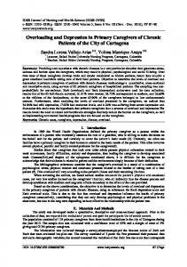
Toutefois la motivation principale de cette thèse réside dans le fait de considérer la surcharge comme une fa¸con d’interpréter l’envoi de message dans la programmation orientée objets. Dans la programmation orienté objets deux fa¸cons distinctes de considérer l’envoi de message coexistent : La première approche considère les objets comme des tableaux qui associent une méthode à chaque message. Lorsque le message m est passé à l’objet obj, la méthode associée à m dans l’objet obj est recherchée. Une telle approche est décrite dans la Figure a. object internal state message 1 method 1 .. .. . . message n

method n

Figure a. Objets comme enregistrements.

message i class name 1 method 1 .. .. . . class name n

method n

Figure b. Messages comme fonctions surchargées.

Ce premier point de vue a été largement étudié et correspond à l’analogie “objets comme enregistrements” introduite dans [Car88] ; dans ce contexte les objets sont des enregistrements (bien sˆ ur!) dont les étiquettes sont les messages et dont les champs contiennent les méthodes correspondantes. L’envoi de message correspond alors à l’extraction de champ. La seconde approche considère les messages comme des identificateurs de fonctions particulières et l’envoi de message comme leur application. Si, dans le contexte des langages typés, nous supposons que le type d’un objet est (le nom de) sa classe alors les messages sont des identificateurs de fonctions surchargées : la méthode est choisie selon la classe (ou, plus généralement, le type) de l’objet auquel le message est passé (voir Figure b). Ainsi nous renversons, dans un certain sens, la situation précédente : au lieu d’envoyer des messages aux objets nous envoyons des objets aux messages. D’emblée, cette deuxième approche semble posséder certains avantages par rapport à la première, au moins sur le plan d’une étude théorique du cas typé. Ceci est vrai en particulier pour les multi-méthodes, le dispatch multiple ou pour l’indépendance logique des donnés persistantes comme dans les langages de programmation pour les bases de données3 . En outre, elle clarifie le rôle de la covariance et de la contra-variance dans la règle de sous-typage pour les méthodes. Par ailleurs, d’autres problèmes surgissent dès que l’on utilise les fonctions surchargées pour modéliser les méthodes. Particulièrement, ceci se produit quand on souhaite intégrer la redéfinition dynamique de nouvelles classes et un haut niveau d’“encapsulation” ; ce dernier point par exemple rend ce formalisme inapte à la modélisation des objets dans les systèmes distribués ` a grand échelle (WADS) pour lesquels les objets doivent encapsuler les méthodes (pour des raisons évidentes de sécurité et d’efficacité). Un regard plus attentif au modèle basé sur la surcharge nous persuade que le style de 3

Dans le sens qu’il est possible d’ajouter des nouvelles méthodes pour les objets d’une classe donnée sans perturber la définition de leurs types et donc le bon typage des applications écrites dans l’ancien schéma

17

CONTENTS

programmation qu’il modélise est tout à fait diffèrent de celui engendré par le modèle basé sur les enregistrements. Le problème est que le terme “orienté objets” regroupe sous un même chapeau de nombreuses techniques différentes. En effet, sous ce terme cohabitent différents styles de programmation dont l’affinité minimale est capturée par les trois termes : “objet”, “envoi de message” et “héritage”. Vouloir pousser plus loin la similarité en incluant d’autres “mots magiques” tels que “encapsulation” ou “modularité” exclurait des classes significatives de langages (e.g. CLOS pour la modularité et Simula pour l’encapsulation). Ces “mots magiques” partitionnent l’ensemble des langages objets en différents styles le composant. La recherche dans le domaine de la théorie des types s’est jusqu’à présent préoccupée de la partition caractérisée par le mot clef “encapsulation des méthodes” et modélisée par les ` partir de [Car88] (déjà paru en 1984) toutes les études théoriques dans le enregistrements. A domaine se fondèrent sur l’hypothèse que les méthodes d’un objet étaient encapsulées dans celui-ci. Ceci excluait des mécanismes tels que les multi-méthodes et le dispatch multiple, présents dans certains langages orientés objets mais pour lesquels ce type de modèles était inadéquat. Au début de notre travail nous pensions que les modèles existants n’était pas assez puissants pour capturer ces mécanismes. C’est pourquoi nous avons commencé à chercher un ` partir des idées de [Ghe91], nous avons établi la base de ce modèle véritablement neuf. A modèle en définissant le λ&-calcul [CGL92b]. Mais portant un regard plus attentif aux mécanismes que nous avions modélisés, nous nous sommes aper¸cu que nous avions décrit un style de programmation complètement différent de celui exposé par les enregistrements. Les modèles par les enregistrements n’étaient pas mis en défaut par celui que nous avions défini mais plus simplement indépendants de celui-ci : à différents mécanismes différents modèles. Le “nouveau” style de programmation orienté objets que nous avons modélisé correspondait ` a celui des fonctions génériques. Il est intéressant de constater qu’à partir d’une approche purement théorique nous avons obtenu un modèle de programmation déjà existant. En fait, nous nous sommes bientˆ ot rendu compte qu’à la relation enregistrement champ étiquette

↔ ↔ ↔

objet méthode message

de l’approche “objets comme enregistrements” correspond la relation fonction surchargée branche

↔ ↔

fonction générique méthode

de notre approche. Dans les deux cas le passage de la théorie à la pratique a permi d’obtenir une discipline de typage (dont la correction peut être formellement prouvée!). Mais comme pour le modèle par enregistrements les bénéfices résultant de la définition d’un modèle typé ne se réduisent pas ` a l’obtention d’une discipline de typage : l’étude du modèle nous suggère d’introduire de nouveaux mécanismes dans les langages orientés objets (par exemple les messages de première classe) ou de généraliser ou redéfinir les mécanismes existants (par exemple les coercitions explicites). Cette thèse est une étude exhaustive de la surcharge combinée à la liaison tardive dans la

18

CONTENTS

perspective particulière de définir ce nouveau modèle, et s’attache également à présenter l’impact pratique qu’un tel modèle peut avoir sur la définition des langages orientés objets et leurs disciplines de types. La thèse est composée de deux parties principales : la première se concentre sur la surcharge pour laquelle la dépendance de types est implicite, dans le sens o` u la sélection de la branche est déterminée par le type de l’argument de la fonction surchargée. La second partie est consacrée ` a l’étude de la dépendance de type explicite de la surcharge, dans le sens o` u la sélection de la branche est déterminée par le type qui est l’argument de la fonction surchargée. Nous détaillons dans les sections suivantes le contenu des chapitres de la thèse.

Programmation orient´ ee objets Un programme orienté objet est construit à partir d’objets. Un objet est une unité de programmation qui associe des données avec les opérations qui peuvent utiliser ou modifier ces données. Ces opérations sont appelés méthodes ; les données sur lesquelles elles opèrent sont les variables d’instance des objets. Les variables d’instance d’un objet sont privées, leur emploi est limité ` a l’objet même : on ne peut y accéder que par les méthodes de l’objet. Un objet est seulement capable de répondre à des messages qui lui sont envoyés ou passés. Un message est le nom d’une méthode définie pour l’objet en question. Le passage de message est le mécanisme de base de la programmation orientée objet. En fait, un programme orienté objets consiste en un ensemble d’objets qui interagissent en s’échangeant des messages. Chaque langage possède sa propre syntaxe pour le passage de message. Nous utilisons la notation suivante : [destinataire message] Le destinataire est un objet ou une expression calculant un objet ; lors de l’envoi d’un message, le système sélectionne entre les méthodes définies pour l’objet en question, celle dont le nom correspond au message ; l’existence de cette méthode doit être vérifiée statiquement (c’està-dire lors de la compilation) par un programme de vérification des types. Nous avons déjà remarqué qu’une manière de comprendre le passage de message est de le considérer comme la sélection d’un champ d’un enregistrement. Dans cette thèse, au contraire, on considère le passage de message comme l’application d’une fonction, o` u le message est (l’identificateur de) la fonction et le destinataire son argument (cette technique est utilisée par les langages CLOS [DG87] et Dylan [App92]). Toutefois les fonctions ordinaires ne suffisent pas à formaliser cette approche. Le fait qu’une méthode appartient ` a un objet spécifique implique que la sémantique du passage de message est tout à fait différente de celle de l’application ordinaire. Deux caractéristiques différencient les messages des fonctions : 1. Surcharge : Deux objets peuvent répondre d’une manière différente au même message. Toutefois tous les objets d’une même classe répondent à un message de la même fa¸con.4 4

Cela n’est pas vrai dans les langages objets basés sur la délégation (delegation based).

19

CONTENTS

Sous l’hypothèse que le type d’un objet est sa classe, cela revient à dire que les messages dénotent des fonctions surchargées, du moment que le code à exécuter est choisi sur la base du type de l’argument. Chaque méthode associée à un message m constitue une branche de la fonction surchargée dénotée par m. 2. Liaison tardive : La deuxième différence entre l’application d’une fonction et le passage d’un message est que la fonction est liée à son exécutable au moment de la compilation, tandis qu’un message est lié ` a la méthode à exécuter seulement pendant l’exécution, lorsque le destinataire est complètement connu. Cette caractéristique, appelée liaison tardive, est un des traits saillants de la programmation orientée objets. Dans notre approche elle naˆıt de la combinaison de la surcharge et du sous-typage. On peut reformuler l’exemple de la section précédente : supposons que les classes Cercle et Carré soient sous-types de la classe Figure et que les trois classes aient une méthode pour le message dessine. Si l’on utilise la liaison précoce, le passage du message suivant λxF igure .(. . . [x dessine] . . . ) est toujours effectué en utilisant la méthode définie pour les figures. En revanche, par liaison tardive la méthode est choisie après que la fonction a été appliquée, selon que x est lié ` a un cercle, ` a un carré ou à une figure. Pour commencer une étude formelle à partir de cette intuition, nous définissons une extension du λ-calcul simplement typé capable de modéliser ces deux mécanismes : surcharge et liaison tardive.

Le λ&-calcul Une fonction surchargée est formée par un ensemble de fonctions ordinaires (i.e. des λabstractions), chacune constituant une branche différente. Pour relier ces fonctions nous avons choisi le symbole & (d’o` u le nom du calcul) ; donc nous enrichissons les termes du λ-calcul simplement typé par le terme suivant : (M &N ) qui, intuitivement, dénote une fonction surchargée avec deux branches, M et N , qui seront sélectionnées selon le type de l’argument. On doit distinguer l’application ordinaire de l’application d’une fonction surchargée, car elles représentent deux mécanismes différents5 . Ainsi nous utilisons “•” pour dénoter une “application surchargée” et “·” pour une application ordinaire. Nous construisons les fonctions surchargées comme des listes, c’est-à-dire en partant d’une fonction surchargée vide dénotée par ε, et en concaténant de nouvelles branches par &. Donc dans le terme précédent M est une fonction surchargée et N une fonction ordinaire (une branche). Ainsi, le terme ((. . . ((ε&M1 )&M2 ) . . . )&Mn ) 5`

A la première est associée une substitution, ` a la deuxième une sélection.

20

CONTENTS

dénote une fonction surchargée avec n branches M1 , M2 , . . . , Mn . Le type d’une fonction surchargée est l’ensemble des types de ses branches. Donc nous ajoutons aux types du λ-calcul simplement typé des ensembles de flèches. Ainsi, si Mi : Ui → Vi alors la fonction surchargée ci-dessus a le type {U1 → V1 , U2 → V2 , . . . , Un → Vn } et si l’on applique cette fonction ` a un argument de type Uj on sélectionnera la branche Mj , soit (0.3) (ε&M1 & . . . &Mn ) • N >∗ Mj · N o` u >∗ signifie “réécrit en zéro ou plusieurs pas”. Nous définissons sur les types une relation de sous-typage. Intuitivement U ≤ V si tout terme de type U peut être utilisé “type safely” là o` u un terme de type V est requis. Donc un calcul ne produira pas d’erreurs de type tant qu’il maintiendra ou réduira les types des termes. La relation de sous-typage pour les types flèches est bien connue (covariance à droite et contra-variance ` a gauche) ; la relation pour les types surchargés est déduite du fait qu’une fonction surchargée peut en remplacer une autre si pour toute branche de la seconde il y en a une de la première capable de la remplacer. Avec le sous-typage, le type de N dans (0.3) peut ne pas correspondre à un des Ui mais être un sous-type de l’un d’entre eux. Dans ce cas on sélectionne la branche dont le type Ui approche au mieux le type U de N , c’est-à-dire on sélectionne la branche j telle que Uj = min{Ui |U ≤ Ui }. Dans notre système les ensembles de flèches ne sont pas tous des types surchargés. En fait un ensemble de types flèche {Ui → Vi }i∈I est un type surchargé si et seulement si pour touts i, j dans I il satisfait les conditions suivantes Ui ≤ Uj

⇒ Vi ≤ Vj

(0.4)

Ui ⇓ Uj

⇒ il existe un unique z ∈ I t.q. Uz = inf{Ui , Uj }

(0.5)

o` u T1 ⇓ T2 dénote l’existence d’un minorant commun pour les types T1 et T2 . La condition (0.4) assure que pendant l’exécution les types ne peuvent que décroˆıtre. Dans un sens elle prend en compte une certaine nécessité de covariance pour les flèches dans la pratique de la programmation. Plus précisément, considérons une fonction surchargée M de type {U1 → V1 , U2 → V2 } o` u U2 < U1 . Si l’on applique M à un terme N ayant à la compilation le type U1 alors le type de M •N lors de la compilation sera V1 . Mais si la forme normale de N a le type U2 (ce qui est tout à fait possible étant donné que U2 < U1 ) alors le type de M •N ` a l’exécution sera V2 et donc la condition V2 < V1 doit être vérifiée. La condition (0.5) concerne la sélection d’une branche. On rappelle que pour l’application d’une fonction de type {Ui → Vi }i∈I à un argument de type U on sélectionne la branche de type Uj → Vj telle que Uj = mini∈I {Ui |U ≤ Ui }. (0.5) est une condition suffisante pour l’existence de ce minimum. Jusqu’à présent nous avons montré comment inclure la surcharge et le sous-typage. Il manque encore la liaison tardive. Une fa¸con très simple de l’obtenir est d’imposer qu’une réduction comme (0.3) ne soit effectuée que si N est fermé et en forme normale.

21

CONTENTS

La description formelle de λ& peut se résumer de la fa¸con suivante : Pr´ e-types V :: = A | V → V | {V1′ → V1′′ , . . . , Vn′ → Vn′′ } Sous-typage La relation de sous-typage est pré-définie sur les types atomiques et elle est étendue aux (pré-)types supérieurs de la fa¸con suivante : ∀i ∈ I, ∃j ∈ J Uj′ → Vj′ ≤ Ui′′ → Vi′′ {Uj′ → Vj′ }j∈J ≤ {Ui′′ → Vi′′ }i∈I

U2 ≤ U1 V1 ≤ V2 U1 → V1 ≤ U2 → V2 Types

1. A ∈ Types 2. si V1 , V2 ∈ Types alors V1 → V2 ∈ Types 3. si pour tout i, j ∈ I (a) (Ui , Vi ∈ Types) et (b) (Ui ≤ Uj ⇒ Vi ≤ Vj ) et (c) (Ui ⇓ Uj ⇒ ∃!h ∈ I . Uh = inf{Ui , Uj }) alors {Ui → Vi }i∈I ∈ Types Termes (o` u V est un type) M :: = xV | λxV .M | M · M | ε | M &V M | M •M Typage [Taut]

[→Intro]

[→Elim≤ ]

xT : T M: T λxU.M : U

ε: {}

[Tautε ]

→T

M: U → T N: W ≤ U M · N: T

[{}Intro]

M : W1 ≤ {Ui → Ti }i≤(n−1) N : W2 ≤ Un → Tn (M &{Ui →Ti }i≤n N ): {Ui → Ti }i≤n

[{}Elim]

M : {Ui → Ti }i∈I N : U Uj = mini∈I {Ui |U ≤ Ui } M •N : T j

o` u tout type apparaissant dans les règles est un type bien formé (i.e. appartient à Type) R´ eduction La réduction > est la fermeture compatible de la notion de réduction suivante : β) (λxT .M )N > M [xT := N ] β& ) Si N : U est clos et en forme normale, et Uj = mini=1..n {Ui |U ≤ Ui } alors {Ui →Ti }i=1..n

(M1 &

M2 )•N >

(

M1 •N M2 · N

for j < n for j = n

22

CONTENTS

Th´ eor` emes Principaux - Elimination de la subsumption : Le langage admet aussi une présentation équivalente avec la règle de subsumption (M : W et W≤ U impliquent M : U ) ´ - Elimination de la transitivité : L’ajout de la transitivité ne modifie pas la relation de sous-typage. - Unicité du type : Chaque terme bien typé possède un seul type - Subject Reduction Généralisée : Soit M : U . Si M >∗ N alors N : U ′ , et U ′ ≤ U . - Confluence : Des termes égaux possèdent un reductum commun. ` ce point il est intéressant de voir comment utiliser en première approximation ce calcul A pour modéliser les langages objets. Tout d’abord il faut noter que dans λ& il est possible d’encoder, soit les paires surjectives (surjective pairings), soit les enregistrements simples (ceux de [Car88]), soit les enregistrements extensibles (voir [Wan87, Rém89, CM91]). Les conditions (0.4) et (0.5) ont dans les langages objets une interprétation très naturelle : supposons que mesg soit l’identificateur d’une fonction surchargée ayant le type suivant mesg : {C1 → T1 , C2 → T2 } Selon la terminologie orientée objet mesg est un message qui dénote deux méthodes, l’une définie dans la classe C1 et retournant le type T1 , l’autre dans la classe C2 et retournant le type T2 . Si C1 est une sous-classe de C2 (plus précisément un sous-type : C1 ≤ C2 ) alors la méthode de C1 masque (overrides) celle de C2 . La condition (0.4) impose alors que T1 ≤ T2 , c’est-à-dire la méthode qui en masque une autre doit retourner un type plus petit. Si par contre C1 et C2 ne sont pas en relation mais qu’il existe une classe C3 sous-classe des deux (C3 ≤ C1 , C2 ) alors C3 a été définie par héritage multiple de C1 et C2 . La condition (0.5) impose qu’une branche soit définie dans mesg pour C3 , c’est-à-dire qu’en cas d’héritage multiple les méthodes définies dans plus d’un ancêtre doivent être redéfinies. Voyons ceci sur un exemple. Considérons la classe 2DPoint avec deux variables d’instance entières x et y, et la classe 3DPoint sous-classe de la première qui possède en plus la variable d’instance z. Ceci peut s’exprimer par les définitions suivantes class 2DPoint { x:Int; y:Int; } : :

class 3DPoint is 2DPoint { x:Int; y:Int; z:Int } : :

o` u à la place des pointillés se trouvent les définitions des méthodes. En première approximation cela peut être modélisé en λ& par deux types atomiques 3DPoint et 2DPoint avec

23

CONTENTS

3DPoint≤2DPoint et dont les types-représentation sont respectivement les types enregistrements hhx : Int; y : Int; z : Intii et hhx : Int; y : Intii. Il faut noter que 3DPoint≤2DPoint est compatible avec le sous-typage des types-représentation correspondants. Une première méthode que l’on pourrait rencontrer dans la définition de 2DPoint est norme = sqrt(self.x^2 + self.y^2) masquée (overriden) dans 3DPoint par la méthode suivante norme = sqrt(self.x^2 + self.y^2 + self.z^2) Dans λ& cela est obtenu par une fonction surchargée avec deux branches p

norme ≡ ( λself 2DP oint . pself.x2 + self.y 2 & λself 3DP oint . self.x2 + self.y 2 + self.z 2 ) dont le type est {2DPoint → Real , 3DPoint → Real}. Il faut noter que self, qui dans les méthodes dénote le destinataire du message, est dans λ& le premier paramètre de la fonction surchargée, i.e. le paramètre dont la classe déterminera la sélection. La covariance apparaˆıt par exemple lorsqu’on définit une méthode qui modifie les variables d’instance. Ainsi, une méthode qui initialise les variables d’instance aura le type suivant initialise : {2DPoint → 2DPoint , 3DPoint → 3DPoint} Supposons que nous ayons défini une nouvelle classe ColorPoint par héritage multiple de 2DPoint et Color et que ces deux classes définissent une méthode efface 6 efface ≡ ( λself 2DP oint .hself ← x = 0i & λself Color .hself ← c = “white”i ) Une telle définition n’est pas bien typée, car {2DPoint → 2DPoint , Color → Color} ne satisfait pas la condition (0.5) ; en réalité en appliquant efface à un objet de classe ColorPoint on ne saurait pas quelle méthode choisir. Par conséquent la condition (0.5) impose l’ajout d’une méthode pour ColorPoint et donc efface : {2DPoint → 2DPoint , Color → Color , ColorPoint → ColorPoint} L’héritage dans ce cadre est donné par le sous-typage plus la règle de sélection des branches : par exemple si l’on applique norme ` a un objet de classe ColorPoint, la méthode exécutée sera celle définie pour 2DPoint. Plus généralement, si l’on passe un message de type {Ci → Ti }i∈I à un objet de classe C la méthode exécutée sera celle définie dans la classe mini=1..n {Ci |C ≤ Ci }. Si ce minimum est exactement C cela signifie que le destinataire utilise la méthode définie dans sa classe ; si le minimum est strictement plus grand que C alors le destinataire utilise la méthode que sa classe, C, a hérité de ce minimum. Il faut noter que la recherche 6

Pour simplifier les exemples nous supposons avoir des conversions implicites entres un type atomique et son type-représentation.

24

CONTENTS

du minimum correspond précisément au “method look-up” de Smalltalk o` u l’on recherche la plus petite super-classe (de la classe du destinataire) pour laquelle une certaine méthode a été définie. L’un des avantages de modéliser les messages par des fonctions surchargées est que, ces dernières étant des valeurs de première classe, les messages sont aussi de première classe. Il devient donc possible d’écrire des fonctions (même surchargées) qui prennent comme argument un message ou le rendent comme résultat. Par exemple on peut écrire la fonction suivante : λm{C→C} . λxC . (m • (m • x)) qui accepte comme argument un message m pouvant être envoyé à un objet de classe C (c’est-à-dire qui a au moins une branche qui puisse travailler avec des objets de classe C), un objet de classe (au moins) C et qui envoie deux fois le message m à l’objet x (bien sˆ ur le résultat du message doit être un objet de classe plus grande que C) Mais l’avantage le plus intéressant d’utiliser cette forme de programmation objet est la possibilité de pouvoir utiliser le dispatch multiple7 : un des problèmes majeurs de l’approche avec enregistrements réside dans l’impossibilité de combiner de manière satisfaisante le soustypage avec les méthodes binaires, c’est-à-dire les méthodes qui ont un paramètre de la même classe que celle du destinataire. Par exemple dans les modèles basés sur les enregistrements les points et les points colorés avec une méthode d’égalité sont modélisés par les enregistrements récursifs suivants : EqP oint ≡ hhx: Int; y: Int; equal: EqP oint → Boolii ColEqP oint ≡ hhx: Int; y: Int; c: String; equal: ColEqP oint → Boolii ` cause de la contra-variance de la flèche le type d’equal dans ColEqPoint n’est pas inférieur ` A a celui d’equal dans EqPoint et donc ColEqPoint6≤EqPoint. Considérons maintenant le même exemple dans λ&. Nous avons déjà rencontré les types atomiques 2DPoint et ColorPoint. On peut continuer ` a les utiliser parce que, contrairement a` ce qu’il se passe avec les enregistrements, l’ajout d’une méthode ` a une classe ne change pas le type des instances. En λ& une définition telle que equal: {2DPoint → (2DPoint → Bool) , ColorPoint → (ColorPoint → Bool)} ne possède pas un type bien formé : ColorPoint≤ 2DPoint donc la condition (0.4) nécessite ColorPoint → Bool ≤ 2DPoint → Bool ce qui n’est pas vrai à cause de la contra-variance de la flèche. Il faut noter qu’une telle fonction choisirait la branche sur la base du type du premier argument seulement. Or, le code de equal ne peut être choisi que dès que l’on connaˆıt les types des deux arguments. C’est pourquoi on ne veut pas accepter le type cidessus (d’ailleurs il serait très facile d’écrire un terme engendrant une erreur). Toutefois dans λ& il est possible d’écrire une fonction qui prenne en compte les types de ses deux arguments pour effectuer la sélection. Pour equal ceci est obtenu de la fa¸con suivante equal: {(2DPoint × 2DPoint) → Bool , (ColorPoint × ColorPoint ) → Bool} 7

C’est-` a-dire la possibilité de sélectionner une méthode en tenant compte de classes autres que celle du destinataire du message

CONTENTS

25

Si l’on passe ` a cette fonction deux objets de classe ColorPoint alors la deuxième branche est choisie ; lorsque l’un des deux arguments est de classe 2DPoint (et l’autre d’une classe plus petite ou égale ` a 2DPoint) la première branche sera choisie. Une autre caractéristique intéressante de ce modèle est qu’il permet d’ajouter une méthode à une classe C déjà existante sans modifier le type de ses objets. En fait, si la méthode doit répondre au message m, il suffit d’ajouter une branche pour le type C à la fonction surchargée dénotée par m. Il est important de noter que la nouvelle méthode est immédiatement disponible pour toutes les instances de C et il est donc possible d’envoyer le message m à un objet de classe C, même si cet objet a été défini avant la branche de m pour C. Cet aspect est très important quand on a ` a gérer des données persistantes, car on peut modifier le schéma logique des donnés (en ajoutant des fonctionnalités) sans devoir modifier les applications déjà écrites. Un des apports de ce modèle est de clarifier les rôles qui jouent la covariance et la contravariance dans le sous-typage (equal en constitue un joli exemple) : la contra-variance est la règle à utiliser lorsqu’on substitue une fonction par une autre de type différent ; la covariance est la règle ` a utiliser lorsqu’on spécialise une branche d’une fonction surchargée par une autre. Il est important de noter que dans ce cas la nouvelle branche ne se substitue pas à l’ancienne branche mais plutôt la masque aux objets de certaines classes. En fait, notre formalisation montre très clairement que la question “contra-variance ou covariance” était un faux problème dˆ u au mélange de deux mécanismes qui n’ont rien à voir l’un avec l’autre : la substitutivité et le masquage. La substitutivité nous indique quand il est possible d’utiliser une expression d’un certain type S a ` la place d’une expression du type T . Cette information est utilisée par l’application : soit f une fonction de type T → U , on veut identifier une catégorie de types dont les valeurs peuvent être passées comme arguments à f ; il faut noter que ces arguments se substitueront dans le corps de la fonction, au paramètre formel qui a le type T . Pour cela nous définissons une rélation de sous-typage telle que f accepte tout argument ayant un type S plus petit que T . La catégorie en question est ainsi l’ensemble des sous-types de T . En particulier, si T est de la forme T1 → T2 il se peut que dans le corps de f le paramètre formel de la fonction soit appliqué à une expression de type T1 ; de ceci on déduit deux choses : le paramètre actuel doit lui aussi être une fonction (donc si S ≤ T1 → T2 alors S doit être de la forme S1 → S2 ), et en plus il doit être une fonction à laquelle on puisse passer des arguments de type T1 (et donc T1 ≤ S1 , eh oui!. . . contravariance). Evidemment, si l’on ne souhaite pas passer des fonctions comme argument, il n’y a aucun sens à définir la relation de sous-typage pour les flèches (c’est pourquoi O2 [BDe92] fonctionne très bien même sans la contra-variance). Le masquage correspond à un tout autre phénomène : on a un identificateur m (en l’occurrence un message) qui identifie par exemple deux fonctions f : A → C et g : B → D (A et B incomparables) ; cet identificateur peut être appliqué à une expression e ; cette application est résolue par le passage de e à f si cette expression a un type plus petit que A (dans le sens de la substitutivité qu’on vient d’expliquer), à g si le type est plus petit que B. Supposons ` a présent que B ≤ A ; la résolution dans ce cas sélectionne f si e a un type compris entre A et B, g si le type de e est plus petit ou égal à B ; mais il y a un problème supplémentaire : les types peuvent diminuer pendant l’exécution ; donc il se pourrait que le type checker voit e de type A et pense que m appliquée à e retournera le type C (f est sélectionnée) ; mais si pendant l’exécution le type de e diminue jusqu’à

26

CONTENTS

B, l’application a le type D ; mais alors D doit être un type qui puisse se substituer à C (dans le sens de la substitutivité plus en haut), i.e. D ≤ C. On peut appeler ceci covariance, si l’on veut, mais il doit être clair qu’il ne s’agit pas d’une règle de sous-typage : g ne se substitue pas ` a f car g ne sera jamais appliquée à des arguments de type A ; g et f sont deux fonctions indépendantes ayant des tˆ aches très précises : f travaille avec les arguments de m ayant un type compris entre A et B, g avec ceux de type plus petit ou égal à B. Il n’est pas question de définir la substitutivité, mais de donner une règle de formation pour un ensemble de fonctions dénoté par un identificateur unique, de fa¸con à assurer la consistance des types pendant l’exécution. D’une fa¸con plus pratique : une méthode a des paramètres ; la classe de chaque paramètre peut ou ne pas être prise en compte pour la sélection de la méthode. Lorsqu’on masque (override) cette méthode, les paramètres dont le type est pris en compte pour la sélection doivent être masqués de manière covariante (i.e. dans la nouvelle méthode les paramètres correspondants doivent posséder un type plus petit), les autres de manière contra-variante (i.e. dans la nouvelle méthode les paramètres correspondants doivent posséder un type plus grand). Dans les modèles basés sur les enregistrements aucun argument est pris en compte pour la sélection : la méthode est déterminée par l’enregistrement dont on sélectionne le champ. Par conséquent, dans de tels modèles il ne peut y avoir que de la contra-variance et le dispatch multiple est impossible. Pour être plus précis, le modèle par enregistrements possède une forme très limitée de covariance mais qui est cachée par le codage des objets : considérons une étiquette ℓ ; pour la règle de sous-typage des enregistrements, si l’on “envoie” cette étiquette à deux enregistrements de types S et T avec S ≤ T alors le type associé à ℓ dans S doit être un sous-type de celui associé ` a ℓ dans T . Cela correspond exactement à notre règle de covariance, mais sa forme est bien plus limitée parce qu’elle ne s’applique qu’aux types enregistrements (puisqu’il s’agit d’un “envoi” d’étiquettes), et non aux produits cartesiens (i.e. dispatch multiple) ni aux flèches.

Normalisation Forte Le λ&-calcul n’est pas fortement normalisant. Cela provient du fait qu’on peut y typer l’auto-application. Considérons le type suivant {{} → T } o` u T est n’importe quel type. Ceci est le type d’une fonction surchargée qui accepte tout argument ayant un type plus petit ou égal à {} (le type surchargé vide). Mais remarquez que tout type surchargé est plus petit que {}, donc en particulier { { } → T } ≤ {}. Dès lors une fonction de type { { } → T } accepte comme argument des termes du même type que le sien et donc soi même ; par conséquent λx{ { }→T } .x•x a pour type { { } → T } → T . Il est donc facile de définir un terme sans forme normale, en imitant les constructions classiques du λ-calcul ; soit ωT

= (ET &{ {}→T , { {}→T }→T } (λx{{}→T } .x•x))

CONTENTS

27

o` u ET est n’importe quel terme clos de type { { } → T } ; le terme ΩT ≡ ωT •ωT qui a type T ne possède pas de forme normale. On peut également définir pour tout type T un opérateur de point fixe YT : (T → T ) → T de la fa¸con suivante YT ≡ λf T →T .((ET &{{}→T,{{}→T }→T } λx{{}→T } .f (x•x))•(ET &{{}→T,{{}→T }→T } λx{{}→T } .f (x•x))) La raison de ce phénomène doit être recherchée dans la définition particulière de la relation de sous-typage. La circularité typique de l’auto-application dérive de la possibilité de pouvoir associer deux types d’une structure syntaxique différente ; plus précisément, deux types ayant des arbres syntaxiques de profondeur différente peuvent être en relation, comme c’est le cas pour {} et {{} → T }. Il est donc possible qu’un type soit sous-type d’une de ses occurrences, d’o` u l’auto-application8 . Toutefois dans notre modélisation de la programmation objet cette forme de circularité n’est jamais utilisée. Il peut donc être intéressant d’étudier des sous-systèmes de λ& qui soient à la fois fortement normalisant et assez expressifs pour modéliser les langages orientés objet. Dans ce but on démontre le théorème suivant : Th´ eor` eme 1 Soit λ&− n’importe quel sous-système de λ& fermé par réduction ; soit rank une fonction associant des entiers aux types de λ&− telle que si T est une occurrence syntaxique de U alors rank(T ) ≤ rank(U ). Si dans λ&− pour toute application M T N U bien typée rank(T ) ≤ rank(U ) alors λ&− est fortement normalisant. Nous qualifions comme stratifiés les systèmes qui satisfont les hypothèses du théorème. Un exemple de système stratifié est obtenu en émondant la relation de sous-typage définie sur les types bien formés de λ& des couples formés par des types de profondeur différente (rank(T ) est dans ce cas la profondeur de l’arbre syntaxique de T ). Ces sous-systèmes sont utilisés pour l’étude de la sémantique.

Trois variations sur le th` eme On peut à ce point étudier comment modifier, étendre ou reformuler λ& pour l’adapter à des exigences spécifiques.

Premi` ere variante : λ&+ La première variante consiste ` a donner plus de liberté à λ& en introduisant certaines modifications qui ont été suggérées en essayant de traduire des langages orientés objets dans λ&. 8

Dans les enregistrements on compare aussi des types d’arbre syntaxique différents, mais les sous-arbres de profondeurs differentes sont toujour séparés par des étiquettes différentes

28

CONTENTS

Tout d’abord la condition (0.5) est trop restrictive pour l’héritage multiple : considérons quatre classes A, B, C et D telles que C et D soient toutes deux sous-types de A et B A B (comme dans la figure ci-contre) ; soit m un message défini dans @ @ les quatre classes, i.e. m: {A → ..., B → ..., C → ..., D → ...}. @ Le domaine de m ne respecte pas la condition (0.5) parce que @ @ A et B n’ont pas de plus petite borne inférieure. Cependant ? R ? @ C D il n’y aura pas d’ambigu¨ıté dans le choix de la branche. Par conséquent, (0.5) est trop restrictive pour modéliser l’héritage multiple tel qu’il est utilisé dans la programmation objets. La condition (0.5) a été introduite pour assurer l’existence d’un minimum pendant la sélection. Toutefois (0.5) est une condition suffisante mais pas nécessaire à l’existence d’un tel minimum. Elle peut donc être améliorée. C’est pourquoi en λ&+ nous rempla¸cons (0.5) par : ∀Ui , Uj ∈ {Ui }i∈I . ∀U élément maximal de LB(Ui , Uj ) ∃!h ∈ I. Uh = U

(0.6)

o` u LB(S, T ) est l’ensemble des bornes inférieures de S et T . Cette condition correspond ` a la gestion de l’héritage multiple, par exemple d’Eiffel. Le théorème suivant démontre qu’il s’agit d’une condition nécessaire et suffisante à l’existence du minimum : Th´ eor` eme 2 Soit (Y, 6) un ensemble partiellement ordonné et, X ⊆ Y . Définissons : (1) ∀a, b ∈ X.∀c ∈ Y. (c élément maximal de LB(a, b) ⇒ c ∈ X) (2) ∀c ∈ Y. {x ∈ X|c 6 x} est soit vide soit possède un plus petit élément alors (1) ⇐⇒ (2) En outre, dans λ&+ on veut avoir la possibilité de remplacer une branche d’une fonction surchargée. Plus exactement si N possède le type U → T et M est une fonction surchargée possédant une branche pour le type U nous souhaitons qu’en écrivant (M &N ) la branche N remplace l’ancienne branche pour U (pourvu que le type obtenu soit bien formé). Il y a plusieurs manières d’obtenir cela. La plus simple est de ne plus imposer dans [{}Intro]

M : W1 ≤ {Ui → Ti }i≤(n−1) N : W2 ≤ Un → Tn (M &{Ui →Ti }i≤n N ): {Ui → Ti }i≤n

que {Ui → Ti }i≤(n−1) soit un type bien formé. De cette fa¸con il devient possible de typer la fonction suivante (M {U1 →T1 ,U2 →T2 ,U3 →T3 } &{U2 →T2 ,U3 →T3 ,U1 →T4 } N U1 →T4 ) même si U1 ≤ U2 , U3 (et donc {U2 → T2 , U3 → T3 } ne peut pas être bien formé). Nous avons déjà vu qu’en λ& il est possible d’ajouter une nouvelle méthode à une classe donnée. Grâce à cette petite modification il devient aussi possible de redéfinir la méthode d’une classe. Enfin, en λ& on effectue la sélection de la branche seulement après que l’argument ait atteint une forme normale fermée. En λ&+ nous voulons pouvoir effectuer la réduction plus tôt, dès que l’on est sˆ ur que toute évaluation ultérieure de l’argument ne changera pas le résultat de la sélection. Dans ce but nous rempla¸cons dans λ&+ la réduction (β& ) par la réduction suivante

29

CONTENTS

+ ) Soit Uj = min{Ui |U ≤ Ui }; si N : U est fermé et en forme normale ou {Ui |Ui ≤ Uj } = β& {Uj } alors ( M1 •N for j < n {Ui →Vi }i=1..n ((M1 & M2 )•N ) > M2 · N for j = n

Autrement dit, dès que l’on a un terme de la forme (M1 &M2 )•N on contrôle s’il y a des branches avec un domaine plus petit que celui de la branche sélectionnée. Si ce n’est pas le cas alors la sélection ne peut plus changer et donc on peut effectuer la sélection, même si N n’est pas clos ou en forme normale. Cette modification est intéressante surtout pour l’optimisation des langages objets a` la compilation. Une règle qui permet de résoudre la sélection d’une méthode ` a la compilation est indispensable pour produire du code efficace. En fait des études préliminaires sur des maquettes du compilateur pour Dylan ont montré qu’en moyenne environ 30% du temps d’exécution d’un code non optimisé est utilisé pour la sélection des méthodes. Résoudre la sélection à la compilation est donc une des nécessités les plus pressantes pour réaliser un langage utilisant des fonctions génériques. Dans λ&+ on + ) pour détecter pendant la compilation les envois de message peut donc utiliser la règle (β& qui peuvent déjà être liés ` a leur méthode. Pour λ&+ nous avons démontré les théorèmes suivants : • Conservativité de la théorie de sous-typage : Si S et T sont deux types bien formés dans λ& alors λ& ⊢ S ≤ T si et seulment si λ&+ ⊢ S ≤ T • Subject Reduction Généralisée : Soit M : U . Si M >∗ N alors N : U ′ , et U ′ ≤ U . • Confluence : Des termes égaux possèdent un réductum commun. • Normalisation forte : Les sous-systèmes stratifiés sont fortement normalisants. Deuxi` eme variante : λ&+coerce La deuxième variante que nous étudions est l’extension de λ& par des coercitions explicites. De manière informelle on peut définir une coercition explicite comme un terme qui change le type de son argument. Par exemple le terme coerceT (M ) change le type de M en T , tout en en conservant les fonctionnalités. Cette construction est une extension cruciale dans λ& o` u les types déterminent l’exécution : le fait de pouvoir changer les types implique un plus grand contrôle sur l’exécution. En particulier il est possible de diriger la sélection sur une branche donnée en appliquant une coercition explicite à l’argument d’une fonction surchargée. De cette fa¸con il devient donc possible de modéliser des commandes telles que as dans Dylan et change-class dans CLOS, dont la fonction est de changer la classe d’un objet. Plus formellement, l’extension par coercitions de λ& est obtenue en ajoutant parmi les termes de λ& le terme suivant coerceT (M ) parmi les règles de typage la règle suivante [Coerce] et parmi les notions de réduction

⊢ M: S ≤ T ⊢ coerceT (M ): T

30

CONTENTS

coerceT (M ) ◦ N > M ◦ N

(coerce)

Il est possible de démontrer que cette extension possède les propriétés suivantes : la conservativité par rapport ` a la théorie équationelle (ou de réduction) des termes ; la subject-reduction généralisée ; la confluence ; la normalisation des sous-systèmes stratifiés. Troisi` eme variante :λ{} Nous voulons définir un système pur de fonctions surchargées, o` u la lambda abstraction soit obtenue comme cas particulier de fonction surchargée avec une seule branche. Il y a donc un seul opérateur d’abstraction et un seul opérateur d’application. La réduction effectuera une sélection et une substitution ` a la fois. Nous utilisons une discipline de sélection semblable ` a + a ne forcer l’appel par valeur que si nécessaire (ainsi le λ-calcul simplement (β& ) de fa¸con ` typé est un sous-calcul de λ{} ). Tout ceci peut être obtenu de la manière suivante : T M Sous-typage (subtype)

::= A | {S1 → T1 , · · · , Sn → Tn } ::= x | λx(M1 : S1 ⇒ T1 , · · · , Mn : Sn ⇒ Tn ) | M M

n≥1 n≥1

∀i ∈ I, ∃j ∈ J Ui′′ ≤ Uj′ et Vj′ ≤ Vi′′ {Uj′ → Vj′ }j∈J ≤ {Ui′′ → Vi′′ }i∈I

Types Tout type atomique appartient ` a Types. Si pour tout i, j ∈ I a. (Ui , Vi ∈ Types) b. (Ui ≤ Uj ⇒ Vi ≤ Vj ) c. (Ui ⇓ Uj ⇒ il existe un seul h ∈ I tel que Uh = inf{Ui , Uj }) alors {Ui → Vi }i∈I ∈ Types Typage [Taut]

Γ ⊢ x: Γ(x)

[Intro]

∀i ∈ I Γ, (x: Si ) ⊢ Mi : Ui ≤ Ti Γ ⊢ λx(Mi : Si ⇒ Ti )i∈I : {Si → Ti }i∈I

[Elim]

Γ ⊢ M : {Si → Ti }i∈I Γ ⊢ N : S Γ ⊢ M N : Tj

Sj = mini∈I {Si |S ≤ Si }

R´ eduction ζ) Soit Sj = mini∈I {Si |U ≤ Si } et Γ ⊢ N : U ; si N est fermé et en forme normale ou {Si |Si ≤ Sj } = {Sj } alors λx(Mi : Si ⇒ Ui )i∈I N >Γ Mj [x: = N ]

31

CONTENTS

Pour cette variante nous avons démontré la propriété de subject réduction généralisée et la confluence. L’intérêt de cette variante est principalement théorique. Toutefois elle n’est pas dépourvue d’intérêt pratique, car elle constitue un premier noyau de calcul basé uniquement sur des fonctions génériques (cf. Dylan).

Un m´ eta-langage de λ& Dans la section consacrée ` a λ& nous avons montré la fa¸con intuitive d’utiliser ce calcul pour modéliser la programmation orientée objets. Toutefois λ& n’est pas adéquat pour une étude des propriétés des langages objets ; il ne possède pas assez de structure pour pouvoir y traduire des “vrais” langages : il manque les commandes pour définir de nouveaux types atomiques, pour travailler sur leur représentation et pour définir la relation de sous-typage ainsi qu’un vrai concept d’objet. C’est pourquoi, nous définissons λ object, un langage minimal directement dérivé de λ&, qui possède ces propriétés, et davantage. En tant que langage, λ object est caractérisé par une sémantique opérationnelle à reduction : cette sémantique est définie pour les termes non typés (dans le sens o` u nous définissons également la sémantique pour les termes qui ne seront pas bien typés) ; ceci nous permet de définir formellement les erreurs de type (en particulier nous distinguons parmi eux l’erreur “message not understood”). Nous définissons ensuite un algorithme de typage et nous en démontrons la correction par rapport à la sémantique opérationelle et ` a la définition d’erreur de type (dans le sens que l’exécution de tout programme bien typé ne cause pas d’erreur de type). L’un des choix critiques dans la définition de λ object est celui de la modélisation des objets. Un objet dans λ object est un terme “taggué” (tagged term). On affecte le “tag” A au terme M par la construction inA (M ) ; l’intuition est que A est la classe de l’objet inA (M ) et M son état interne. Ainsi par exemple in2DP oint (hx = 0; y = 0i) est un objet de la classe 2DPoint dont les variables d’instance x et y ont la valeur 0. Les tags (i.e les classes) doivent être déclarés en les associant au type de leur état interne (ceci sert pour le typage). Par exemple, pour la classe 2DPoint ceci est obtenu par : let 2DPoint hide hhx : int, y : intii in . . . Dans un certain sens une telle déclaration correspond à la définition dans ML d’un “datatype” de la forme : datatype 2DPoint = in2DP oint of {x : int, y : int} Plutôt que d’utiliser le filtrage comme dans ML nous utilisons, pour accéder à l’état interne d’un objet, une fonction out qui composée avec in donne l’identité. Il faut aussi déclarer un ordre sur les tags. Cet ordre, qui correspond à l’ordre de “sous-classe”, est à la fois utilisé pour la résolution de la surcharge et pour le typage : let ColorPoint ≤ 2DPoint, Color in . . . Les fonctions surchargées ne peuvent avoir comme argument que des objets ou des produits d’objets (dispatch multiple). La description des types, des expressions et des programmes du langage est donnée par les productions suivantes, o` u A dénote un tag :

32

CONTENTS

T

::= A | T × T | T → T |

M

P

{(A1 × . . . × Am1 ) → T1 , . . . , (A1 × . . . × Amn ) → Tn }

::= xT | λxT.M | M · M

|

n,mi ≥1

ε | M &TM | M •M

|

< M , M > | π1 (M ) | π2 (M ) | µxT .M

|

coerceA (M ) | superA (M ) | inA (M ) | outA (M )

::= M | let A ≤ A1 , ... , An in P | let A hide T in P

S´ emantique op´ erationnelle Un autre aspect important de λ object est la définition des valeurs tagguées : une valeur tagguée est tout terme qui, passé ` a une fonction surchargée, permet immédiatement la sélection de la branche. Une bonne définition des valeurs tagguées est très importante parce que, + ) (cf. page 28), elle est le meilleur moyen pour effectuer des opticouplée avec la règle (β& misations ` a la compilation. Nous utilisons GD pour dénoter une valeur tagguée par le tag D.9 A2 An 1 GD : : = inD (M ) | coerceD (M ) | superD (M ) | < GA 1 , G2 , . . . , Gn > Avant de donner la sémantique opérationelle nous devons encore définir la notion de valeur dans λ object, c’est-à-dire distinguer les termes qui peuvent être considerés comme des résultats. Nous utilisons la méta-variable G pour dénoter les valeurs G ::= x | (λxT .M ) | ε | (M1 &TM2 ) | < G1 , G2 > | coerceA (M ) | superA (M ) | inA (M ) La sémantique opérationnelle est donc définie par les règles suivantes (nous utilisons ◦ pour dénoter soit · soit • et D pour le mini=1..n {Di |C ⊢ D ≤ Di }) : Axiomes (C (C (C (C (C (C (C (C (C (C (C 9

, , , , , , , , , , ,

πi (< G1 , G2 >) ) ⇒ ( C , Gi ) i=1,2 outA1 (inA2 (M )) ) ⇒ ( C , M ) outA1 (coerceA2 (M )) ) ⇒ ( C , outA1 (M ) ) outA1 (superA2 (M )) ) ⇒ ( C , outA1 (M ) ) µx.M ) ⇒ ( C , M [x := µx.M ] ) (λx.M ) · N ) ⇒ ( C , M [x := N ] ) (M1 &{D1 →T1 ,...,Dn →Tn } M2 )•GD ) ⇒ ( C , M1 •GD ) if Dn 6= D {D →T ,...,D D D n →Tn } 1 1 • (M1 & M2 ) G ) ⇒ ( C , M2 · G ) if Dn = D and GD 6≡ superD (M ) {D →T ,...,D D n →Tn } 1 1 (M1 & M2 )•G ) ⇒ ( C , M2 · M ) if Dn = D and GD ≡ superD (M ) let A ≤ A1 . . . An in P ) ⇒ ( C ∪ (A ≤ A1 ) ∪ . . . ∪ (A ≤ An ) , P ) let A hide T in P ) ⇒ ( C , P )

Dans la dernière production D ≡ (A1 × . . . × An ); donc un tag peut être aussi le produit de plusieurs types atomiques. Nous utilisons le non terminal D pour les produits de types atomiques.

33

CONTENTS

Règles de contexte ( C , M ) ⇒ ( C , M′ )

( C , M ) ⇒ ( C , M′ )

( C , ) ⇒ ( C , )

( C , ) ⇒ ( C , )

( C , M ) ⇒ ( C , M′ )

( C , M ) ⇒ ( C , M′ )

( C , πi (M ) ) ⇒ ( C , πi (M ′ ) )

( C , outA (M ) ) ⇒ ( C , outA (M ′ ) )

( C , M ) ⇒ ( C , M′ )

( C , M ) ⇒ ( C , M′ )

( C , M ◦ N ) ⇒ ( C , M′ ◦ N )

( C , (N1 &N2 )•M ) ⇒ ( C , (N1 &N2 )•M ′ )

L’application ordinaire est implémentée par un appel-par-nom, tandis que l’application d’une fonction surchargée est réalisée par un “appel-par-valeur-tagguée”. Syst` eme de types Nous sommes ` a present capables de donner la définition d’erreur de type. Un programme produit une erreur de type s’il se réduit à une forme normale qui n’est pas une valeur. En particulier si l’exécution est bloquée sur un terme de la forme ((M1 &T M2 )•GD ) nous disons que l’erreur produite est “message not understood”. Il faut noter que dans ce dernier cas la réécriture a échoué parce que D (i.e. mini=1..n {Di |C ⊢ D ≤ Di }) n’est pas défini : ceci peut dériver soit du fait que l’ensemble {Di |D ≤ Di , i = 1..n} est vide (ceci signifie que nous avons envoyé un message au mauvais destinataire) soit du fait qu’il n’y a pas de plus petit élément (ceci signifie que la condition sur l’héritage multiple n’a pas été respectée). Il nous reste ` a définir un système de types qui assure qu’un programme bien typé ne produit pas d’erreurs de type. Le système de type en question est très semblable à celui de λ&+ (parce que nous voulons pouvoir modéliser l’héritage dans sa forme la plus générale et l’extension/redéfinition de méthode). La différence la plus importante est qu’il doit prendre en compte les déclarations pour les tags introduites par (let A ≤ . . . in ) et (let A hide . . . in ). Ceci est fait par les règles suivantes : [NewType]

[Constraint]

[Coerce] [Super] [In] [Out]

C , S[A ← T ] ⊢ P : U C, S ⊢ let A hide T in P : U C ∪ (A ≤ Ai )1=1..n , S ⊢ P : T C, S ⊢ let A ≤ A1 , ... , An in P : T C, S ⊢ M : B C, S ⊢ coerceA (M ): A C, S ⊢ M : B C, S ⊢ superA (M ): A C, S ⊢ M : T C, S ⊢ inA (M ): A C, S ⊢ M : B C, S ⊢ outA (M ): S(A)

A 6∈ dom(S), T ∈C,S Types and T not atomic if C ⊢ S(A) ≤ S(Ai ) and A do not appear in C

C ⊢ B ≤ A and A ∈C,S Types C ⊢ B ≤ A and A ∈C,S Types C ⊢ T ≤ S(A) and A ∈C,S Types C ⊢ B ≤ A and A ∈C,S Types

34

CONTENTS

On peut donc prouver que si un programme est bien typé alors il ne produit pas d’erreurs de type. Le langage λ object ainsi défini peut alors être utilisé pour prouver des propriétés des langages objets. Dans le chapitre de la thèse dédié à λ object nous définissons un langage fonctionnel objets simple o` u l’on retrouve les constructions usuelles (class, super, self, new, héritage multiple etc.) et d’autres moins usuelles (messages de première classe, extension/redéfinition de méthodes, multi-méthodes mutuellement récursives)10 ; nous définissons aussi une discipline de types pour ce langage. Puis nous donnons une traduction de ce langage dans λ object et en définissons ainsi la sémantique. Enfin nous démontrons que la traduction d’un programme bien typé est un terme bien typé dans λ object et obtenons, de cette fa¸con, une preuve de correction de la discipline de types définie pour ce langage objets simple . Pour terminer nous montrons comment il est possible, sous certaines hypothèses, de coder λ object dans λ&+ . L’implémentation en Caml Light d’un interpreteur pour λ object est décrite en Appendix A.

S´ emantique La définition d’une sémantique pour λ& présente quatre problèmes principaux: pré-ordre, exécution dépendant des types, liaison tardive, imprédicativité. Plus précisément : • Pré-ordre : La relation de sous-typage dans λ& est un pré-ordre. En fait soit U ≤ V , alors par les règles de sous-typage de λ& on obtient que {U → T, V → T } ≤ {V → T } et {V → T } ≤ {U → T, V → T }. Toutefois ces deux types sont complètement interchangeables : on peut utiliser l’un ou l’autre dans un programme sans que rien ne change. Nous voulons par conséquent qu’ils aient la même interprétation, et donc que “≤” soit interprété par une relation d’ordre entre les types sémantiques. • Exécution dépendant des types : les types des termes déterminent le résultat de l’exécution. Par conséquent l’interprétation d’une fonction surchargée doit prendre en compte l’interprétation du type de son argument. • Liaison tardive : L’interprétation d’une application surchargée doit être déterminée par le type de l’argument ` a l’exécution, lorsque cet argument aura atteint une forme normale fermée. • Imprédicativité : nous avons déjà montré dans la section sur la normalisation forte que la relation de sous-typage ne respecte pas la taille des types ; c’est pourquoi il est possible d’appliquer une fonction de type { {} → T } à elle même. Nous venons de dire que l’interprétation d’une fonction doit prendre en compte l’interprétation du type de son argument. Par conséquent l’interprétation du type { {} → T } fait appel ` a l’interprétation du type lui même, d’o` u l’imprédicativité! Pour traiter le problème du pré-ordre nous utilisons la construction syntaxique dite de “complétion”. Un type surchargé {U → T } possède en effet un nombre (potentiellement infini) 10

voir Appendix C.1

35

CONTENTS

de branches virtuelles, une pour chaque sous-type de U . La complétion d’un type surchargé est son expansion par ces branches virtuelles. Donc par exemple la complétion de {U → T } sera {U → T, U1 → T, U2 → T, . . . } o` u U1 , U2 , ... forment l’ensemble des sous-types de U . Plus formellement, on change la notation des types surchargés de manière à pouvoir écrire des types infinis. Nous écrivons ⇓ H, si l’ensemble de types H possède une borne inférieure. D´ efinition 1 Un type surchargé généralisé (t.s.g.) est un couple (K, out) o` u K est un ensemble de types et out est une fonction de K vers Types telle que 1. si H ⊆ K et ⇓ H alors il existe V ∈ K tel que V ∈ inf H.11 2. out est monotone par rapport au pré-ordre de sous-typage. Parfois on utilisera {U → out(U )}U ∈K pour dénoter le t.s.g. (K, out) Il faut noter que tout type surchargé est un t.s.g. mais pas nécessairement le contraire. Nous pouvons maintenant définir la complétion. Nous complétons un t.s.g. en élargissant son domaine par les sous-types des types dans le domaine et en étendant la fonction out au c out) d o` domaine ainsi élargi. En d’autres termes, la complétion de (K, out) est le t.s.g. (K, u ′ ′ ′ ′ c d K = {U |∃U ∈ K U ≤ U } et out(U ) = out(min{U ∈ K|U ≤ U }). L’interprétation d’un type surchargé sera l’interprétation de sa complétion, et ainsi nous obtiendrons que deux types équivalents (c’est-à-dire tels que l’un soit plus petit que l’autre et vice-versa) aient la même interprétation, puisqu’il est possible de prouver qu’ils ont la même complétions. La sémantique est donnée dans un modèle (D, ·) du λ-calcul sans type : les termes sont interprétés par des (classes d’équivalence d’) éléments du modèle et les types par des relations partielles d’équivalence sur le modèle même. En outre, pour tenir compte du fait que l’exécution dépend des types, nous codons l’ensemble des types syntaxiques, Types par un sous-ensemble [Types]⊆ D du modèle12 . Il y a donc une dualité dans l’interprétation syntaxique d’un type : type comme ensemble de valeurs qui est interprété par une relation partielle d’équivalence, et type comme valeur déterminant l’exécution qui est interprété comme élément du modèle dans [Types]. La dépendance est alors obtenue en interprétant un type surchargé par un produit indexé sur les codes des types syntaxiques. Plus précisément, si l’on écrit Td pour le type syntaxique associé à l’élément d dans [Type], la sémantique d’un type surchargé est donnée par [[{U → out(U )}U ∈K ]] =

Y

d n )]] [[Tn → out(T

b n∈[K]

c = {d | Td ∈ K}. c A ` ce point on cerne mieux d’o` o` u [K] u surgit le problème de l’imprédicativité : considérons une fois de plus le type { {} → T } et soit d son codage dans [Types] ; son interprétation sera un produit indexé sur les codes des sous-types de {}, i.e. sur les codes de tous les types surchargés. Par conséquent, parmi les index du produit il y aura d lui même. Donc l’interprétation du type ci-dessus, c’est-à-dire [[Td ]] est donné en termes de [[Td ]] → [[T ]]. Cette 11

La plus grande borne inférieure dans le pré-ordre est une classe d’équivalence La seule restriction que l’on impose est que la topologie induite sur [Type] soit la topologie discrète, afin que toute fonction dans [Types] → D puisse être étendue ` a une fonction continue dans D → D 12

36

CONTENTS

forme d’impédicativité est similaire a` celle que l’on trouve dans le Système F : la sémantique de ∀X.T est le produit indexé sur la sémantique de tous les types et, donc, sur ∀X.T lui même. Dans les relations partielles d’équivalence, par exemple, le problème est résolu en indexant le produit sur l’ensemble PER de toutes les relations partielles d’équivalence : [[∀X.T ]]E =

Y

[[T ]]E[X:=C]

C∈PER

Cette définition est bien fondée car PER existe indépendamment des types qui y sont interprétés. De fa¸con semblable dans F≤ on interprète ∀X ≤ S.T par le produit indexé sur les sous-relations de l’interprétation de S : [[∀X≤ S.T ]]E =

Y

[[T ]]E[X:=C]

C⊆[[S]]E

Dans notre système nous ne sommes pas capables d’imiter ces constructions parce que nous sommes forcés d’indexer les produits sur un “codage” des types, qui donc n’existe pas de manière indépendante des types mêmes. Il nous est ainsi impossible de définir dans le modèle un ordre des codes qui respecte l’ordre de sous-typage. Autrement dit, dans les modèles de F≤ il est possible de définir un ordre ⊆ tel que si S ≤ T alors [[S]] ⊆ [[T ]]. Ici nous ne sommes pas capables de trouver dans le modèle un ordre 4 sur les éléments de D tel que si Tn ≤ Tm alors n 4 m. Donc nous ne sommes pas capable de donner la sémantique du système complet. C’est pourquoi, les définitions de cette section s’appliquent uniquement aux sous-systèmes stratifiés, pour lesquels on ne rencontre pas ce problème d’imprédicativité. Le fait que le calcul soit dépendant des types se manifeste dans la définition de la sémantique d’une fonction surchargée. Soit (M1 &M2 ) de type {U → out(U )}U ∈K ; son interprétation doit être un élément d’un produit indexé sur le codage des types. Plus précisément c et Uj = min{U ∈ [[(M1 &M2 )]] est la fonction f qui pour tout code d d’un type dans K K|Td ≤ U } est définie de la fa¸con suivante : f (d) =

(

[[M2 ]] si Uj sélectionne la deuxième branche [[M1 ]](d) sinon

L’interprétation d’une fonction surchargée est un élément d’un produit indexé ; elle est donc une fonction dans le modèle qui prend comme argument le code d’un type et restitue un élément (une classe d’équivalence) dans le type sémantique approprié. Ainsi l’interprétation de l’application d’une fonction surchargée est donnée par [[M •N ]] = ([[M ]](d))[[N ]]

(0.7)

Avec la liaison tardive d doit être le codage du type de la forme normale fermée de N . Or, il est impossible connaˆıtre ce type sans exécuter N et le contexte dans lequel cette expression se trouve. D’autre part, il n’est pas possible d’effectuer cette exécution pour donner l’interprétation car on perdrait la compositionalité de la définition. On pourrait envisager d’utiliser ` a la place de d (le codage d’) une variable de type, mais ainsi on entrerait dans le domaine d’un calcul du second ordre que nous ne maˆıtrisons pas encore. Donc nous

37

CONTENTS

nous limitons au cas de liaison précoce. Dans ce but nous modifions la définition des termes de λ& de la manière suivante : M :: = xV | λxV .M | M · M | coerceV (M ) | ε | M &M | M •coerceV (M ) ainsi nous sommes sˆ urs que le type de l’argument d’une fonction surchargée ne pourra plus changer pendant l’exécution, car il est contraint (coerced) à un type donné. Par conséquent “d” dans (0.7) est le code associé au type de N . Pour cette sémantique on peut démontrer les théorèmes suivants : • Correction par rapport au sous-typage : Si U ≤ V est dérivable alors [[U ]] ⊑ [[V ]] (⊑ inclusion entre relations partielles d’équivalence comme ensembles de couples) • Correction par rapport au typage : Si N : U est dérivable alors [[N ]] ∈ [[U ]]. (relation comme ensemble de classes d’équivalence) • Correction par rapport a ` la réduction : Si M >N alors [[M ]] ⊇ [[N ]]. (classe d’équivalence comme ensemble d’éléments de D)

Second ordre Dans la section précédente nous évoquions la possibilité d’étudier un formalisme du second ordre afin de mieux cerner la signification mathématique de la liaison tardive. Une telle étude couvrirait un thème qui, jusqu’à présent, a été négligé par la recherche, soit, l’étude du polymorphisme dans un calcul o` u l’exécution dépendrait directement des types. Le Système F de Girard [Gir72] est un calcul o` u l’on peut définir des fonctions qui prennent des types comme argument ; néanmoins ces fonctions dépendent de leurs arguments d’une fa¸con très limitée : des types différents comme argument n’affectent que le type du résultat, pas sa valeur. La contrepartie pratique de cette propriété est que les types peuvent être effacés pour l’exécution, qui est ainsi effectuée sur les effacements (erasures) des termes. F≤ est une extension conservative de F qui permet de plus de spécifier des bornes pour les paramètres de type. Cependant il possède encore la même forme de dépendance des types que F , car les types peuvent être effacés pour l’exécution. En revanche, nous somme intéressés en une dépendance de types qui affecte l’exécution. Nous voulons pouvoir décrire des fonctions qui exécutent (dispatch) des codes différents en fonction du type passé comme argument. Cette recherche se situe donc dans un cadre plus général : elle vise la formalisation du polymorphisme explicite dit “ad hoc” [Str67] ainsi que son intégration avec sa contrepartie : le polymorphisme paramétrique. Toutefois il y a d’autres motivations qui amènent à s’intéresser au second ordre, et dont la retombée pratique immédiate est bien plus importante. Il s’agit de résoudre le problème qui dans la recherche théorique sur les systèmes de types pour les langages à objets est dénommé “le problème de perte d’information”. Ce problème a été présenté dans [Car88] sur une observation de Antonio Albano et peut être illustré de la manière suivante. Considérons la règle d’application du λ-calcul simplement typé avec sous-typage: [→Elim≤ ]

M: T → U N: S ≤ T MN: U

38

CONTENTS

et deux types S et T tels que S ≤ T ; par exemple soit S un type enregistrement comme T mais avec des champs supplémentaires. Prenons la fonction d’identité pour T , λxT .x qui possède donc le type T → T . Soit M un terme de type S. Par la règle ci-dessus (λxT .x)M a le type T (plutôt que S). Nous avons ainsi perdu de l’information; dans l’exemple des enregistrements on a perdu l’information liée aux champs supplémentaires de S car, après avoir appliqué M ` a l’identité, il n’est plus possible d’avoir accès à ces champs. La solution ` a ce problème consiste à passer à un formalisme du second ordre, et a été originairement décrite dans [CW85]. L’idée en elle même est très simple : l’identité ci-dessus n’est plus une fonction qui accepte tout argument de type plus petit ou égal à T et rend un résultat de type T , mais elle devient une fonction qui accepte tout argument de type plus petit ou égal ` a T et rend un résultat du même type que celui de l’argument. Autrement dit, la fonction identité possède le type ∀X≤ T.X → X. 13 On rencontre un problème analogue dans λ&. Soit m un message qui modifie l’état interne des objets de la classe C1 . Puisque nous sommes dans un cadre fonctionnel la méthode dans C1 rend un nouvel objet de classe C1 . Par conséquent m: {..., C1 → C1 , ...}. Soit C2 une sous-classe de C1 qui hérite la méthode en question. Si l’on passe le message m à un objet de classe C2 la branche définie dans C1 va être sélectionnée. Mais cette branche possède le type C1 → C1 , par conséquent le résultat du passage du message aura le type C1 au lieu de C2 . Nous utilisons pour λ& la même solution que pour le problème de [Car88] et passons à l’étude de formalismes du second ordre avec sous-typage. Plus particulièrement, notre recherche se concentre sur F≤ qui est considéré comme la formalisation standard de la quantification bornée. Nous agissons tout d’abord sur deux plans : nous essayons d’améliorer F≤ et, parallèlement, de l’étendre par la surcharge et la liaison tardive. Après avoir réuni ces deux études, nous montrons comment le polymorphisme “ad hoc” explicite peut être utilisé pour modéliser la programmation objets.

Vers une quantification born´ ee d´ ecidable Les systèmes avec quantification bornée sont obtenus en enrichissant le Système F par une relation de sous-typage et un type Top (le type plus grand que tous les types) et en spécifiant une borne pour toute variable quantifiée. Les règles d’introduction et d’élimination des types polymorphes sont étendues de manière à prendre en compte ces bornes. La formulation standard de la quantification bornée, F≤ , a été définie par Curien et Ghelli [CG92]. Parmi les règles de sous-typage celle qui permet de comparer les types polymorphes possède la forme suivante : (∀-orig)

C ⊢ T1 ≤ S1 C ∪ {X ≤ T1 } ⊢ S2 ≤ T2 C ⊢ ∀(X≤ S1 )S2 ≤ ∀(X≤ T1 )T2

X 6∈ dom(C)

Cette règle peut être lue de la fa¸con suivante. Un type T de la forme ∀(X≤ T1 )T2 décrit une collection de termes polymorphes (fonctions qui prennent un type et rendent un terme) qui 13

Ce genre de polymorphisme peut être soit de forme explicite (la quantification est linguistique : X est substitué par le type explicitement passé ` a la fonction) soit de forme implicite (la quantification est métalinguistique : X est substitué par le type trouvé par unification par le système de typage).

39

CONTENTS

associent des sous-types de T1 ` a des termes dans T2 . Si T1 est un sous type de S1 , alors le domaine de T est plus petit que celui de ∀(X≤ S1 )T2 ; ainsi ce dernier a une contrainte plus faible et décrit une plus grande collection de termes polymorphes. En outre, si l’on considère un type S = ∀(X≤ S1 )S2 tel que pour tout U qui soit un argument recevable par les fonctions des deux collections (i.e. par celles avec la contrainte plus restrictive : U ≤ T1 ), la U -instance de S2 est un sous-type de la U -instance de T2 alors T est “par points” une contrainte plus faible que S et il décrit donc une plus grande collection de termes polymorphes. Bien que sémantiquement très naturelle, cette règle est à l’origine de la perte de maintes propriétés syntaxiques désirables. Tout d’abord elle cause l’indécidabilité de la relation de sous-typage [Pie93, Ghe93a], ce qui entraˆıne l’indécidabilité du contrôle des types. Mais pire encore, F≤ ne possède pas de plus grande borne inférieure pour les ensembles bornés de types, ce qui empêche certains raisonnements par induction ou, plus simplement, le typage d’un “if then else” possédant deux branches dont les types soient incomparables (mais avec un minorant commun). Le cœur du problème réside dans la borne pour la variable X de S2 : cette borne est S1 dans la conclusion de la règle, et devient T1 dans la prémisse droite. Ce “re-liage” des variables, en lui même assez bizarre, invalide toute une classe de raisonnements par induction structurelle sur les types, o` u le cas pour une variable utilise normalement l’hypothèse d’induction sur la borne. C’est pourquoi plusieurs variantes de cette règle ont été proposé dans la littérature. La règle originaire proposée par Cardelli et Wegner dans [CW85] pour leur calcul Fun (voir (∀Fun) Figure 0.1) évite ce reliage en limitant la comparaison à des types ayant la même borne ;

(∀-Fun)

C ∪ {X≤ U } ⊢ S2 ≤ T2 C ⊢ ∀(X≤ U )S2 ≤ ∀(X≤ U )T2

(∀-local)

C ⊢ T 1 ≤ S1 C ∪ {X≤ S1 } ⊢ S2 ≤ T2 C ⊢ ∀(X≤ S1 )S2 ≤ ∀(X≤ T1 )T2

Figure 0.1: Règles alternatives quoique décidable cette restriction ne possède aucune motivation sémantique apparente et elle empêche la modélisation des types partiellement abstraits (voir [CP94]). Katiyar et Shankar [KS92] proposent une restriction dans laquelle les bornes ne peuvent par contenir Top. De cette fa¸con on obtient la décidabilité mais aux frais de l’expressivité du calcul car les enregistrements (dont le codage dans F≤ utilise Top) ne peuvent plus être utilisés comme bornes. Une autre variation, (∀-local), utilise la borne la plus grande pour comparer les corps des quantifications (voir Figure 0.1). Mais Giorgio Ghelli a montré récemment qu’elle est impraticable d’un point de vu algorithmique, tout en laissant ouvert le problème de la décidabilité. Nous proposons une alternative très simple : une règle de sous-typage pour la quantification universelle (∀-new)

C ⊢ T1 ≤ S1 C ∪ {X≤ Top} ⊢ S2 ≤ T2 C ⊢ ∀(X≤ S1 )S2 ≤ ∀(X≤ T1 )T2

X 6∈ dom(C)

o` u les corps des quantifications doivent être reliés (S2 ≤ T2 ), mais sous aucune hypothèse

40

CONTENTS

(refl)

C ⊢T ≤T

(Top)

C ⊢ T ≤ Top

(trans)

C ⊢ T1 ≤ T2 C ⊢ T2 ≤ T3 C ⊢ T1 ≤ T3

(→)

C ⊢ T 1 ≤ S1 C ⊢ S2 ≤ T 2 C ⊢ S1 → S2 ≤ T 1 → T 2

(taut)

C ⊢ X ≤ C(X)

(∀)

C ⊢ T 1 ≤ S1 C ∪ {X≤ Top} ⊢ S2 ≤ T2 C ⊢ ∀(X≤ S1 )S2 ≤ ∀(X≤ T1 )T2

Figure 0.2: Relation de sous-typage pour F≤⊤ préalable (X≤ Top). Cette règle est d’un point de vu sémantique plus naturelle que les autres variantes puisqu’elle concrétise une notion de sous-typage “par points” que l’on retrouve dans d’autres travaux [Mit90b, BM92, Bru93, PT93] : elle affirme, tout simplement, que ∀F ≤ ∀G (o` u F, G : Type→Type) si et seulement si dom(G) ⊆ dom(F ) et F est “par points” plus petit que G. ´ Evidement, cette règle est plus faible que (∀-orig). Le système obtenu de F≤ en rempla¸cant (∀-orig) par (∀-new), et que nous appelons F≤⊤ (voir Figure 0.2), ne peut pas prouver une un jugement tel que ⊢ ∀(X ≤ S1 )X ≤ ∀(X ≤ S2 )S2 qui est au contraire prouvable dans F≤ . Toutefois cette différence d’expressivité ne joue aucun rôle dans les cas d’application pratique de la quantification bornée. En fait, nous avons testé cette règle avec le modèle de programmation orientée objets présenté dans [PT93], qui utilise l’extension de F≤ par le polymorphisme d’ordre supérieur du Système F ω [Gir72] : tout terme de ce modèle possède dans F≤⊤ le même type que dans F≤ . De même, Luca Cardelli nous a confirmé que tout programme écrit pour son implémentation de F≤ [Car93], est aussi typable dans F≤⊤ . Une autre application de la quantification bornée est donnée par la traduction due à Cardelli d’un calcul d’enregistrements extensibles dans F≤ [Car92] : une fois de plus, F≤⊤ peut être utilisé à la place de F≤ . F≤⊤ possède plusieurs propriétés syntaxiques qui font défaut à F≤ . En premier lieu le sous-typage est décidable. En fait il est possible de définir un algorithme de sous-typage qui est valide (sound) et complet (complete) par rapport à F≤⊤ ; ceci est obtenu en démontrant pour F≤⊤ les propriétés d’élimination de la réflexivité et de la transitivité, et la terminaison de l’algorithme qui en dérive14 . La décidabilité du sous-typage est une propriété assez souhaitable. Cependant, d’un point de vu pratique, son absence cause moins de troubles que la non existence du plus grand minorant et du plus petit majorant. Giorgio Ghelli [Ghe90] a montré que F≤ présente une telle carence. Par contre dans F≤⊤ toute paire de types possède un plus petit majorant et tout paire de type avec un minorant commun possède un plus grand minorant. La simplicité syntaxique accrue de la formalisation de F≤⊤ entraˆıne une remarquable simplification des preuves par rapport a` F≤ . Cette simplification, nous la rencontrons tant dans les preuves de validité et complétude de l’algorithme de sous-typage qu’en étudiant la sémantique de F≤⊤ . Pour donner une sémantique à F≤⊤ il est possible d’utiliser la technique 14

Un récent résultat non encore publié de Giorgio Ghelli prouverait que cet algorithme peut être implémenté de manière polynˆ omiale.

41

CONTENTS

de [BTCGS91], et ainsi traduire F≤⊤ dans un calcul avec des coercitions explicites pour lequel plusieurs modèles sont déjà définis. Grâce à l’existence des plus grandes bornes inférieures et des plus petites bornes supérieures, il est possible d’utiliser cette même technique pour donner une sémantique ` a l’extension de F≤⊤ qui comprend les types enregistrements, les types récursifs et les types énumérés (variant types), technique qui, dans le cas de F≤ , échoue. Si nous étendons le langage des types de F≤ par les types récursifs (µX.T ) et ajoutons parmi les règles de sous-typage (Unfold-l)

C ⊢ S[X := µX.S] ≤ T C ⊢ µX.S ≤ T

(Unfold-r)

C ⊢ T ≤ S[X := µX.S] C ⊢ T ≤ µX.S

la théorie de sous-typage ainsi obtenue n’est pas une extension conservative de la théorie pour F≤ . Autrement dit, il existe un jugement de sous-typage dans F≤ qui n’est pas prouvable avec le système originel mais qui est prouvable par la théorie étendue [Ghe93b]. Donc l’algorithme de contrôle des types obtenu en ajoutant à l’algorithme pour F≤ les deux règles ci-dessus, n’est pas correct. Par contre si nous étendons F≤⊤ de la même manière —appellons ce système F≤⊤µ — nous obtenons une extension conservative de la théorie de sous-typage. Ceci découle très simplement de la démonstration d’élimination de la transitivité pour F≤⊤µ (propriété qui n’est pas satisfaite dans l’extension de F≤ ).15 Par conséquent, nous pouvons étendre l’algorithme de sous-typage pour F≤⊤ par les deux règles ci-dessus ; nous obtenons ainsi un algorithme de sous-typage pour F≤⊤µ qui est valide, complet et qui termine. Comme nous l’avons montré, le passage de la règle (∀-orig) à la règle (∀-new) apporte de nombreux bénéfices au système de sous-typage, qui dès lors satisfait plusieurs propriétés souhaitables. Malheureusement, ce même passage a un effet néfaste sur la relation de typage. En fait, comme Giorgio Ghelli l’a fait remarquer, F≤⊤ ne possède pas la propriété d’existence d’un type minimal, dans le sens o` u l’ensemble des types prouvés par un terme donné peut ne pas posséder de plus petit élément. Ceci est illustré par l’exemple suivant: considérons le terme M ≡ ΛX≤ Y.λxX. x. En utilisant la règle de subsumption, il est possible de prouver que ce terme est typé tant par le type ∀(X≤ Y )X → X que par type ∀(X≤ Y )X → Y . Ces deux types sont tous les deux minimaux dans l’ensemble des types de M . En conséquence, si dans l’algorithme de typage habituel pour F≤ nous utilisons l’algorithme de sous-typage pour F≤⊤ , nous obtenons un algorithme de typage qui est valide pour F≤⊤ , mais qui n’est pas complet. Par exemple, l’algorithme de typage déduira pour M ci-dessus le premier type mais pas le second. Le problème de trouver un algorithme de typage complet dans ce cas demeure ouvert, comme demeure ouvert le problème de la décidabilité de la relation de typage. C’est l’interaction entre la règle de subsumption, et la règle (∀-new) qui est responsable de la perte de cette propriété. En fait, en utilisant la subsumption nous pouvons faire remonter dans la hiérarchie de sous-typage, le type du corps d’une Λ-abstraction, alors que la règle (∀-new) empêche l’algorithme de sous-typage de faire la même chose. Toutefois, il faut noter que les tests que nous avons effectués sur les interpréteurs existants de F≤ , ont consisté ` a 15 En fait, si T1 et T2 sont deux types de F≤ , et si T1 ≤ T2 est faux dans F≤ mais est prouvable dans l’extension par les types récursifs, alors il existe un type récursif T tel que T1 ≤ T ≤ T2 soit prouvable dans l’extension. Ceci n’est pas possible dans F≤⊤µ : si c’était le cas, par l’élimination de la transitivité on obtiendrait une preuve de T1 ≤ T2 sans utiliser la transitivité. Mais la preuve ainsi obtenue serait aussi une preuve de T1 ≤ T2 dans F≤⊤ : ce qui est impossible.

42

CONTENTS

remplacer dans l’algorithme de sous-typage la règle (∀-orig) par la règle (∀-new), mais tout en continuant ` a utiliser l’algorithme de typage traditionnel. Ainsi, aucune utilisation de la règle de subsumption n’a été faite. On pourrait être tenté de continuer à adopter la philosophie consistant ` a éliminer des jugements inutiles (sous tendant l’entière définition de F≤⊤ ) et, donc, considérer comme relation de typage celle définie par la composition de l’algorithme de typage de F≤ , et la nouvelle relation de sous-typage. Cependant un autre problème surgit: le système résultant ne satisfait pas la propriété de subject reduction. Considérons le terme ΛX ≤ Y.λy Y . (λxX. x)y. Le type déterminé pour ce terme par l’algorithme de typage est ∀(X ≤ Y )Y → X. Le terme en question se réduit en un pas à ΛX ≤ Y.λy Y . y pour lequel l’algorithme de typage rend ∀(X≤ Y )Y → Y , qui est incomparable (pour la règle (∀-new) ) avec le type précédent. Maintenant, considérons ce même système dans lequel les réductions à l’intérieur des Λabstractions ne sont pas utilisées; nous éliminons ainsi non seulement d’“inutiles” jugements de typage et de sous-typage mais encore d’“inutiles” réductions. Pour un tel système, dont le typage est décidable (évident, car tout terme bien type possède un seul type, celui déterminé pas l’algorithme) et dont la relation de sous-typage possède toutes les bonnes propriétés établies dans cette section, nous conjecturons la propriété de subject-reduction. Notons que c’est ce système que nous avons implicitement testé en utilisant les implementations de Cardelli et de Pierce et Turner de l’algorithme de typage de F≤ avec la relation de sous-typage modifiée

Quantification born´ ee avec surcharge Nous avons déjà montré qu’une méthode qui modifie l’état interne d’un objet de classe C1 m: {..., C1 → C1 , ...} possède le même problème de perte d’information que la fonction identité de type C1 → C1 : dans les deux cas en passant un argument de type strictement plus petit que C1 , on obtient un résultat de type C1 . La solution adoptée pour la fonction identité était de passer à un formalisme du second ordre et d’utiliser ainsi le type ∀X≤ C1 .X → X. Comme nous l’avons déjà anticipé, nous adoptons pour λ& la même solution. Donc l’idée est de définir un système de types o` u le message m ci-dessus puisse avoir un type de la forme m: {..., ∀X≤ C1 .X → X, ...} u cette dépendance des types est traitée de fa¸con C’est pourquoi, nous définissons F≤& o` explicite. Dans un langage de programmation une fonction qui prend comme argument un type et qui pour chaque type exécute un code différent, aurait très probablement la syntaxe suivante : Fun(X:*) = if X≤T1 then exp 1 else if X≤T2 then exp 2 else . . . if X≤Tn then exp n

43

CONTENTS

Cette fonction exécute l’expression exp1 si on lui passe un type plus petit ou égal à T1 , exp2 si le type passé est plus petit ou égal à T2 et ainsi de suite. S’il y a plus d’un candidat possible on sélectionne parmi eux la branche avec la borne la plus petite. Dans F≤& nous dénotons cette fonction par : (ΛX≤ T1 .exp1 & ΛX≤ T2 .exp2 & . . . & ΛX≤ Tn .expn ) Pour des raisons techniques nous quantifions un type surchargé à l’extérieure de ses parenthèses ; ainsi le type de la fonction ci-dessus sera : ∀X{T1 .S1 , T2 .S2 , . . . , Tn .Sn } o` u expi : Si . Comme pour λ& nous avons deux conditions pour sélectionner les types bien formés. La première est une condition de cohérence qui assure que le type diminue toujours, même si au cours de l’exécution on change la branche sélectionnée. Ceci était donné dans λ& par la condition de covariance (0.4). La condition correspondante dans le second ordre impose pour un type surchargé ∀X{Ti .Si }i∈I que pour tout i, j ∈ I si C ⊢ Ti ≤ Tj alors C ∪ {X≤ Ti } ⊢ Si≤ Sj . La deuxième condition doit assurer pour la sélection l’existence d’une branche avec une borne minimum (entre les branches compatibles avec l’argument). Pour le second ordre il ne suffit plus d’imposer que pour tout couple de bornes compatibles Ti et Tj dans ∀X{Ti .Si }i∈I il existe une borne qui en est le plus grand majorant. Le problème est que les bornes peuvent contenir des variables libres. Donc il faut contrôler les conflits pour toute valeur admissible pour ces variables. Pour assurer l’existence de la branche sélectionnée nous imposons deux restrictions : tout d’abord les bornes ne peuvent qu’être soit des types atomiques (des noms de classe) soit des variables bornées par des types atomiques. Ceci nous permet d’éviter tout problème dˆ u` a la contra-variance des types flèche. En outre, on demande que les bornes d’un type surchargé satisfassent la condition dite de “∩-closure” (meet-closure) qui est définie comme suit : soit A un type atomique ou une variable bornée par un type atomique; dénotons par B(A) le type A lui-même dans le premier cas et la borne de la variable A dans le second. La ∩-closure impose que pour tout Ai et Aj dans ∀X{Ai .Si }i∈I si B(Ai )⇓B(Aj ) alors il existe h dans I tel que Ah est la plus grande borne inférieure de Ai et Aj . Si {Ai }i∈I satisfait cette condition (assez restrictive) alors pour tout type T et pour toute substitution σ compatible avec les bornes des variables libres dans {Ai }i∈I l’ensemble {σ(Ai ) | T ≤ σ(Ai ), i ∈ I} est soit vide soit possède un plus petit élément. On définit donc le système de types de F≤& en ajoutant aux productions des types de F≤ la production suivante T : : = ∀X{Ai .Ti }i∈I en ajoutant aux règles de sous-typage de F≤ la règle suivante: ({ })

pour tout i ∈ I il existe j ∈ J t.q. C ⊢ A′i≤ Aj C ∪ {X≤ A′i } ⊢ Tj ≤ Ti′ C ⊢ ∀X{Aj .Tj }j∈J ≤ ∀X{A′i .Ti′ }i∈I

X 6∈ dom(C)

Ensuite nous utilisons la relation de sous-typage ainsi définie pour sélectionner les types qui sont bien formés, c’est-à-dire les (pré-)types qui satisfont la covariance, la ∩-closure et dont les bornes ne prennent comme valeurs que des types atomiques.

44

CONTENTS

Nous démontrons pour ce système la cohérence du sous-typage, ainsi que les propriétés d’élimination de la réflexivité et de la transitivité. De ce dernier résultat découle une présentation algorithmique de la relation de sous-typage. L’algorithme ainsi obtenus est une procédure de semi-décision : F≤& , hérite de F≤ l’indécidabilité du sous-typage. Les termes de F≤& sont obtenu en ajoutant aux productions des termes de F≤ les productions suivantes : a: : = ε | (a&I a) | a[A] o` u a[A] indique l’application d’une fonction surchargée (pour la différencier de l’application d’une fonction polymorphe que nous notons par a(T )) et I un index de la forme [A1 .T1 k . . . k An .Tn ]. Les index sont utilisés pour la sélection et le typage. Les nouveaux termes sont typés de la fa¸con suivante : C ⊢ ε: ∀X{}

[ε]

[{}Intro]

C ⊢ a: T1≤ ∀X{Ai .Ti }i≤n C ⊢ b: T2≤ ∀(X≤ A)T C ⊢ (a&[A1 .T1 k...kAn .Tn kA.T ] b): ∀X({Ai .Ti }i≤n ∪ {A.T }) C ⊢ a: T

[{}Elim]

C ⊢ Aj = mini∈I {Ai |C ⊢ A≤ Ai } C ⊢ a[A]: Tj [X := A]

B(T )= ∀X{Ai .Ti }i∈I

Ces règles vont s’ajouter ` a celles du typage pour les termes de F≤ . La cohérence du typage dérive directement de la cohérence du sous-typage. Enfin nous augmentons les notions de réduction de F≤ par la règle suivante : (β{} ) Si A, A1 . . . , An sont fermés alors C ⊢ (a&

[A1 .T1 k...kAn .Tn ]

b)[A] >

(

b(A) si An = min1≤i≤n {Ai |C ⊢ A≤ Ai } a[A] sinon

La condition de fermeture des types utilisés pour la sélection correspond à l’utilisation de la liaison tardive pour ce calcul. Le calcul ainsi défini satisfait les propriétés de subject-réduction généralisée et de confluence. Nous conjecturons que F≤& est aussi fortement normalisant. Nous avons vu qu’en rempla¸cant dans F≤ la règle de sous-typage pour la quantification universelle par la règle (∀-new) nous obtenons un système de sous-typage décidable. Il est donc légitime de se poser la question de savoir si en effectuant le même changement dans a la fois possède un sous-typage décidable et soit assez expressif F≤& on obtient un calcul qui ` pour modéliser la programmation orientée objets. La réponse est affirmative : en fait on ne rencontre aucun problème particulier à reparcourir les preuves de F≤⊤ de terminaison du sous-typage et d’élimination de la transitivité pour le système ainsi obtenu. Il est intéressant de noter que la décidabilité est obtenue par la seule modification de la règle (∀), tandis que la règle de sous-typage ({}) pour les types surchargés demeure inchangée. En effet, on pourrait s’attendre ` a ce que la borne dans la prémisse de droite de la règle ({})

45

CONTENTS

a Top. Ceci n’est pas nécessaire pour la décidabilité : en fait, les doive être changée de A′i ` bornes utilisées dans la quantification surchargée sont de loin moins générales que celles de la quantification universelle, car dans ces dernières Top peut y apparaˆıtre, d’o` u l’indécidabilité (dans un certain sens les types surchargés de ce système—que nous notons F≤&⊤ —forment un système qui satisfait la restriction de [KS92]). Nous conjecturons que F≤⊤ hérite de toutes les bonnes propriétés de la relation de soustypage de F≤⊤ , en particulier l’existance d’une plus grand borne inférieure et d’une (unique) plus petite borne supérieure. Ce qui est certain c’est que ce système possède toutes les mauvaises propriétés de F≤⊤ , notamment il ne satisfait pas la proprieté d’existance d’un type minimal et le système sans la règle de subsumption, ne satisfait pas la propriété de “subjectreduction”. Cependant, si la conjecture posée à la fin de la section précédente est correcte elle impliquera automatiquement la même propriété pour F≤&⊤ , c’est-à-dire que le système, sans la règle de subsumption et sans réductions impliquant des variables libres de type, satifera non seulment la décidabilité mais encore la propriété de subject-reduction.

Surcharge de second ordre et programmation orient´ ee objets Nous allons maintenant montrer comment utiliser le formalismes du second ordre que nous avons défini dans la séction précédente, pour la modélisation des langages objets. Tout les examples de cette section sont typables tant dans F≤& que dans F≤&⊤ (sans ou avec subsumption). Comme dans la section sur λ& nous utilisons des types atomiques pour les noms des ` chaque type atomique est associé un type-représentation qui décrit les variables classes. A d’instance de la classe. Une relation de sous-typage peut être définie sur ces types atomiques, pourvu qu’elle respecte le sous-typage des types-représentation. Une fois de plus, un message est un identificateur de fonction surchargée ; mais cette fois la méthode ` a exécuter est choisie sur la base du type passé comme argument, qui sera la classe de l’objet auquel le message est envoyé. Ainsi l’envoi du message mesg à un objet a de classe A est modélisé par (mesg[A])a. Une fois de plus nous considérons les types atomiques 3DPoint et 2DPoint avec 3DPoint ≤ 2DPoint (les types-représentation sont toujours les mêmes). Le message norme devient donc norme ≡ ( ΛMytype≤ 2DPoint .λself & ΛMytype≤ 3DPoint .λself )

p

.pself.x2 + self.y 2 M ytype . self.x2 + self.y 2 + self.z 2 M ytype

dont le type est ∀Mytype.{2DPoint.M ytype → Real, 2DColorPoint.M ytype → Real} Nous avons utilisé la variable self pour dénoter, à l’intérieur d’une méthode, le destinataire du message et, en conformité avec la notation de [Bru92], la variable Mytype pour dénoter le type du destinataire. Il faut noter que contrairement à [Bru92] nous n’avons pas besoin de récursion.

46

CONTENTS

Le message d’initialisation aura dans F≤& le type suivant : initialise : ∀M ytype{2DP oint.M ytype → M ytype, 3DP oint.M ytype → M ytype} qui est bien formé (il satisfait de manière triviale les conditions de bonne formation). Mais même si nous avions défini initialise de fa¸con qu’il aie le type initialise : ∀M ytype{2DP oint.M ytype → 2DP oint, 3DP oint.M ytype → M ytype} nous aurions encore obtenu un type bien formé. En fait, la condition de covariance demande que {M ytype≤ 3DP oint} ⊢ M ytype → M ytype ≤ M ytype → 2DP oint ce qui est vrai dans ce cas. Plus généralement, si le message m a été défini dans les classes Bi (pour i ∈ I) alors le type de m a la forme ∀Mytype{Bi .M ytype → Ti }i∈I . Si Bh ≤ Bk alors la méthode définie pour m dans la classe Bh a masqué (overridden) celle définie dans ´ Bk . Etant donné que Mytype est le même dans les deux branches (c’est ici que se justifie le fait d’utiliser un unique quantificateur pour toutes les branches), la condition de covariance se réduit ` a prouver que {M ytype≤ Bh } ⊢ Th ≤ Tk et donc que la méthode masquante rend un type plus petit ou égal à celui de la méthode masquée. L’exemple avec initialise montre pourquoi il est important de vérifier cette condition sous l’hypothèse que Mytype soit plus petit que la borne la plus petite. Au contraire si une méthode rend un résultat de type Mytype alors une méthode la masquant doit aussi retourner un résultat de type Mytype (et pas le nom de la classe o` u la méthode a été définie parce que par héritage ceci pourrait être un type plus grand que la valeur actuelle de Mytype). L’intérêt du second ordre réside dans l’élimination du problème de perte d’information : ceci avait lieu pour le message efface de la page 23. En fait si l’on envoyait ce message ` a un objet de classe 3DP oint le résultat de l’envoi avait le type 2DP oint. Par contre dans le second ordre la branche pour 2DPoint dans efface aura la définition suivante : efface ≡ ( ΛMytype ≤ 2DPoint.λself

M yT ype

.hself ← x = 0i & . . . )

dont le type est ∀Mytype.{2DPoint.Mytype → Mytype, . . . } L’envoi du message efface ` a un objet b de type 3DPoint est traduit en (efface [3DPoint])(b). Pour les règles [{}Elim] et [→Elim] cette expression possède le type 3DPoint ; nous n’avons donc pas de perte d’information. Comme pour λ& la redéfinition ou l’ajout d’une méthode correspondent a` la concaténation d’une nouvelle branche ` a une fonction surchargée. De même, les messages sont des valeurs de première classe ; un exemple trivial d’utilisation de cette propriété est donné par la définition d’une fonction qui envoie un message à self en commen¸cant la recherche de la méthode de la classe C (ceci ressemble ` a la fonction super) : let super C = λm∀X{C.T } .m[C]self Cette fonction accepte comme argument tout message pouvant être envoyé à un objet de

47

CONTENTS

classe C (l’expression est bien typée pourvu que Mytype ≤ C). Il faut noter que la possibilité d’appliquer les termes aux types, donne un plus grande contrôle sur le calcul, tout comme l’introduction des coercitions explicites l’avait donné dans λ&. Le calcul que nous venons de décrire est assez simple, surtout à cause des restrictions sur les bornes d’une fonction surchargée. Toutefois il n’y a aucune difficulté à modifier la définition de ∩-closure pour permettre comme bornes des produits cartésiens de classes (pour modéliser le dispatch multiple) et des structures d’ordre autres que le demi-treillis (pour modéliser l’héritage multiple dans toute sa généralité : voir la condition (0.6) page 28). Il est intéressant toutefois de noter qu’en cas de dispatch multiple la condition de covariance a une signification différente qu’en λ&. Nous rappelons qu’en λ& le message equal ne pouvait pas être typé par {2DP oint → 2DP oint → Bool, 2DColorP oint → 2DColorP oint → Bool} car ce dernier n’est pas un type bien formé. C’est pourquoi, dans λ& nous définissions equal : {(2DP oint × 2DP oint) → Bool, (2DColorP oint × 2DColorP oint) → Bool} Par contre, en passant au second ordre le type ∀X{2DP oint.X → X → Bool, 2DColorP oint.X → X → Bool} est bien formé. Toutefois pour sélectionner la branche correcte il faut passer entre les types des deux arguments celui qui est le plus grand. Ceci n’est pas ce qu’on voudrait : on aimerait passer ` a la fonction les deux types des arguments et laisser au système la tâche de sélectionner la branche correcte. Ceci peut être obtenu par des multi-méthodes, en définissant equal de sorte qu’elle possède le type suivant : ∀X{2DP oint × 2DP oint.X → Bool, 2DColorP oint × 2DColorP oint.X → Bool} F≤& ne capture pas la puissance de tous les langages orientés objets ; cependant il possède certaines caractéristiques qui leur manquent. Donc on peut envisager d’enrichir les langages existants par ces caractéristiques ; par exemple on pourrait définir un nouveau langage ` a objets qui fournisse soit la paramétricité soit la surcharge, o` u les classes puissent être passées comme argument aux fonctions ; ces fonctions pourraient alors exécuter des codes différents selon la classe re¸cue comme argument. On peut imaginer plusieurs applications d’un tel mécanisme : par exemple, imaginons de devoir écrire une routine générale d’installation pour des logiciels qui travaillent sur des machines différentes. Imaginons de classifier les logiciels en mathématiques et graphiques, et les machines en machines noir et blanc et machines couleur. Très probablement cela correspondrait aux classes suivantes : GraphSW, MathSW≤ Software et Color, B&W≤ Machine et la routine d’installation aura le type install : ∀(M≤ M achine)∀(S≤ Software )(M × S) → . . . Le corps de cette routine inclura certaines parties communes à toutes les machines et à tous les logiciels, et certaines parties spécialisées selon l’espèce des arguments. Cette spécialisation sera obtenue en utilisant des fonctions de type : ∀X{Software × M achine. ..., GraphSW × B&W. ..., GraphSW × Color. ..., M athSW × B&W. ..., M athSW × Color. ...}

48

CONTENTS

Parmi les limites de modélisation du second ordre ou, plus précisément, de la ∩-closure il faut citer l’impossibilité de modéliser les classes génériques du langage Eiffel [Mey88]. Une classe est générique quand elle est paramétrée par une variable de type. Par exemple, si X est une variable de type, alors nous aimerions pouvoir définir une classe Stack[X] avec deux méthodes pop: X et push: X → (), et puis obtenir une pile d’entiers en instantiant X de la manière suivante : new(Stack[Int]). Il ne semble pas être trop difficile d’affaiblir la définition de ∩-closure pour permettre parmi les bornes des fonctions surchargées des constructeurs monotones de types. Mais nous n’avons pas d’idée simple pour traiter les constructeurs nonmonotones. Toutfois ceci n’est pas une limite de l’approche, mais seulment de sa formalisation actuelle.

Conclusion Nous concluons cette présentation en situant notre travail dans un contexte plus général et en suggérant les perspectives de notre recherche future. Th´ eorie de la Preuve Au début de ce chapitre nous avons rappelé la classification introduite par [Str67], subdivisant le polymorphisme entre “ad hoc” et paramétrique. Ce dernier est à son tour réparti en polymorphisme (paramétrique) implicite, o` u la quantification des types est une opération méta-linguistique qui exprime l’utilisation de schémas de types dans la théorie de la preuve correspondante [Hin69, Mil78], et en polymorphisme (paramétrique) explicite o` u cette même quantification est exprimée par un opérateur linguistique et o` u la multiplicité des instances “prouvées” par un terme est linguistiquement exprimée par un unique type syntaxique [Gir72, Rey83]. Nous introduisons pour le polymorphisme “ad hoc” la même classification, mais avec un sens légèrement différent : nous définissons comme implicite le polymorphisme “ad hoc” o` u la sélection de la branche est basée sur le type de l’argument ; nous définissons comme explicite le polymorphisme “ad hoc” o` u la sélection de la branche est basée sur le type passé en argument. L’emploi de la même terminologie que pour le polymorphisme paramétrique est justifié par le fait que le polymorphisme ad hoc implicite peut être caractérisé par une quantification méta-linguistique sur les (sous-types des) “types d’entrée” d’une fonction surchargée, tandis que dans le polymorphisme ad hoc explicite cette quantification est promue au niveau linguistique. Ceci devient encore plus évident si l’on utilise la notation des types surchargés généralisés introduite ` a la page 35 ; le type surchargé {Ui → out(Ui )}i∈I peut être considéré comme une notation alternative du schéma de type suivant : d} .α → out(α) d ∀α ∈ {U i i∈I

(0.8)

Ainsi un terme de type {Ui → out(Ui )}i∈I est implicitement polymorphe dans le sens o` u il possède plusieurs types obtenus en instanciant le schéma (0.8). Pour typer l’application d’une d} .α → out(α) d fonction M : ∀α ∈ {U on utilisera une instance particulière de son schéma : i i∈I

49

CONTENTS

[{}Elim]

d ) M : U → out(U N: U d ) M •N : out(U

Il faut noter que la variable générique α peut varier sur l’ensemble des sous-types des types d’entrée. Ceci se manifeste au niveau linguistique dans le traitement de la sémantique par la notion de complétion : la quantification méta-linguistique est transformée en l’expansion de ses instances, afin d’être interprétée comme un produit indexé sur les types. Nous pouvons donc classifier les différents calculs sur la base de la présence et du type éventuel des différentes formes de polymorphisme. Nous nous trouvons donc en présence de neuf classes de langages, dont certaines (dénotées par (1) et (2) ) sont vides :

λ-calc. simplement typé λ&-calcul (1) ML ML+ fonctions génériques (2) Système F(≤) λ&+F(≤) F≤&

polymorphisme param´ etrique ad hoc absent absent absent implicite absent explicite implicite absent implicite implicite implicite explicite explicite absent explicite implicite explicite explicite

Il faut noter que les deux formes de polymorphisme sont syntaxiquement distinguées car elles sont implémentées par des termes différents; ainsi dans la table ci-dessus chaque colonne se réfère à la caractéristique du calcul pur des termes correspondant (car dès que l’on introduit le polymorphisme ad hoc, le système ne satisfait plus la paramétricité dans le sens de [MR91, Rey83]). Enfin, le lecteur ne devrait pas être étonné que la table ci-dessus mélange calculs avec et sans sous-typage : en fait, tous les calculs que nous avons étudiés possèdent le sous-typage (car cela implique un gain remarquable en puissance expressive). Toutefois cette classification est également valable pour les langages sans sous-typage ; et pour adapter cette étude à ces langages il suffit d’utiliser l’égalité syntaxique pour le sous-typage (i.e. S ≤ T ⇔S ≡ T ), avec toutes les simplifications que cela entraˆıne. Programmation orient´ ee objets Nous avons déjà remarqué tout au long de cette présentation que notre modèle donne des fondements ` a un style de programmation orientée objets différent de celui modélisé par les enregistrements. C’est pourquoi ce modèle est capable de capturer aisément des mécanismes différents et d’en suggérer d’autres totalement nouveaux. Nous avons aussi montré que le fait d’étudier “le revers de la médaille” nous a permis de mieux cerner le fonctionnement des modèles à enregistrements (tel est le cas pour la covariance/contra-variance) ainsi que leurs limites.

50

CONTENTS

Nous voulons conclure ce point par quelques mots sur l’héritage, car dans cette thèse nous avons limité notre étude uniquement à la forme d’héritage qui dérive de l’utilisation du soustypage. En effet, dans la programmation objets le sous-typage et l’héritage caractérisent deux hiérarchies différentes, bien que très liées l’une à l’autre. Le sous-typage concerne l’exécution des expressions, puisqu’il établit dans quel cas les expressions d’un type donné peuvent être utilisées l` a o` u une expression d’un type différent est attendue. L’héritage se rapporte à la définition des opérations pour les expressions d’un type donné car il établit dans quel cas les expressions d’un type donné peuvent utiliser certaines opérations initialement définies pour un type différent. Selon cette définition le sous-typage implique l’héritage car si les expressions d’un type donné peuvent se substituer ` a celles d’un autre type alors ils peuvent aussi utiliser toute opération définie pour ce type. Toutefois la réciproque n’est pas vérifiée car dans certains cas on peut avoir la réutilisation du code mais pas la substitutivité. Ce dernier point est illustré simplement par la méthode qui effectue la copie du destinataire 16 : class C {...} copy = self [[ copy: Mytype ]] ´ Evidement le code de copy peut être utilisé par n’importe quelle classe, mais ceci n’implique pas que toute classe puisse être un sous-type de C. Si l’on ne dispose que du sous-typage, et que l’on souhaite définir une nouvelle classe C’ entièrement différente (pour l’état interne) de C mais possédant une méthode copy, alors la seule solution possible est de redéfinir à nouveau copy dans C’. Si, au contraire, l’on possède un mécanisme général d’héritage alors il devient possible d’exprimer que C’ hérite (de tous les codes) des méthodes de C. Ceci peut s’écrire de la fa¸con suivante : class C’ is ... inherits from C {...} : : o` u C’ hérite de C sans en être sous-type. Ceci peut intuitivement être modélisé dans F≤& en admettant parmi les bornes d’une fonction surchargée les types union. Par exemple la méthode copy ci-dessus pourrait être modélisée par l’expression suivante : copy ≡ (ε&ΛMytype ≤ C ∪ C ′ .λselfM ytype.self) : ∀Mytype{C ∪ C ′ .Mytype → Mytype} Le type union indique que la branche en question est partagée par C et C ′ . Cette branche sera sélectionnée chaque fois que, lors de l’application de copy à un type A, l’un de ces deux types (C ou C ′ ), se trouvera être le plus petit des types supérieurs apparaissant dans une borne. Il est nécessaire donc de vérifier séparément la branche pour chaque type, i.e. X≤ C ⊢ a: T X≤ C ′ ⊢ a: T ⊢ ΛX≤ C ∪ C ′ .a: ∀(X≤ C ∪ C ′ )T 16

Pour une explication precise de la notatio utilisée, voir le chapitre 1

51

CONTENTS

Ainsi, ∪ dénote un “ou-exclusif” plutôt que l’union. Il est important de noter que dans ce cas l’héritage est un mécanisme spécifique à une opération dont le code doit être partagé ; ceci n’implique pas le partage de toute opération définie pour le type concerné. Donc dans notre formalisme nous pouvons introduire une nouvelle forme d’héritage, partiel, dont la caractéristique est qu’un type hérite seulement de certaines opérations définies pour un autre type. L’écriture class C’ is . . . inherits from C en haut indiquait que C’ héritait de toute opération définie pour C. Mais par héritage partiel nous pouvons spécifier que C’ n’hérite de C que de la méthode copy (et de rien d’autre). Une syntaxe possible pourrait être: class C’ is ... {...} copy = inherited from C [[ .. .]] Dans ce cas la définition de copy dans F≤& donnée ci-dessus est encore valable. Il faut remarquer que cet héritage partiel est impossible dans les modèles par enregistrements o` u toutes les méthodes d’une classe doivent obligatoirement être héritées. Cette nouvelle vue de l’héritage nous suggère une autre généralisation de ce mécanisme. Jusqu’à présent l’héritage a été restreint aux classes (i.e. aux types atomiques). Or, il n’y a aucune raison apparente de ne limiter les unions qu’aux types atomiques. Par exemple en F≤& nous pourrions envisager d’admettre des bornes formées par l’union de produits de types atomiques, obtenant d’emblée l’héritage pour les multi-méthodes. Mais des unions de types encore plus générales pourraient être étudiées. Pour compléter cette étude on pourrait envisager d’introduire des types intersection ` a l’intérieur des bornes. Ceci permettrait de définir de manière aisée une condition de ∩-closure pour types d’ordre supérieur, ce qui nous permettrait de modéliser les classes génériques. Au del` a de la programmation objets Dès le début nous avons affirmé que la combinaison de la surcharge et de la liaison tardive permet un très haut niveau de programmation incrémentale et de réutilisation du code. Ces caractéristiques ne sont pas, et ne doivent pas être, une exclusivité de la programmation orientée objets. C’est pourquoi il devient très intéressant d’essayer de les exporter à d’autres paradigmes, moyennant l’introduction de la surcharge et de la liaison tardive. Au moment de la rédaction de cette thèse nous avons déjà commencé à appliquer ces mécanismes aux langages des modules ; plus précisément nous sommes en train d’étudier une extension du système de modules de SML par des foncteurs surchargés combinés avec la liaison tardive. Toutefois il n’y a pas de limite apparente à l’application de ces techniques, et une extension à d’autres paradigmes (systèmes concurrents ou programmation logique, par exemple) peut également être envisagée.

52

CONTENTS

Introduction a quien leyere: Si las paginas de este libro consienten alg´ un verso feliz, perd´ oneme el lector la descortes´ıa de haberlo usurpado yo, previamente. Nuestras nadas poco difieren; es trivial y fortuita la circustancia de que seas t´ u el lector de estos ejercicios, y yo su redactor Jorge Luis Borges Fervor de Buenos Aires (1923)

An important distinction has been extensively used in language theory for the last two decades, between parametric (or universal) polymorphism and “ad hoc” polymorphism [Str67] (see also [CW85]). Parametric polymorphism allows one to write a function whose code can work on different types, while using “ad hoc” polymorphism it is possible to write a function which executes different code for each type. Both the Proof Theory and the semantics of the first kind of polymorphism have been widely investigated by many authors, on the grounds of early work of Hindley, Girard, Milner and Reynolds, and developed into robust programming practice. The second kind, usually known as “overloading”, has had little theoretical attention, with the notable exception of [WB89], [MOM90] and [Rou90]; consequently, its wide use has been little affected by any influence comparable to the one exerted by implicit and explicit polymorphism in programming. This is due, probably, to the fact that the traditional languages offer a very limited form of overloading: in most of them only predefined functions (essentially arithmetic operators defined on integers and reals and input/output operators) are overloaded, while in the relatively few languages where the programmer can define overloaded functions their actual meaning is always decided at compile time. This form of overloading can be easily understood as a form of syntactic abbreviation which does not significantly affect the underlying language. Indeed we understand that the real gain of power with overloading happens only when one computes with types: to exploit the whole potentiality of overloading, types must be computed during the execution of the program and the result of this computation must affect the final “value” of the whole execution. Overloading resolution performed at compile time does not operate any computation on the types; the selection of the code to execute is nearly reduced to a macro expansion. It is true that in languages with a “classic” type discipline, delaying to run time the choice of the code to execute would not have any effect, since types do not change during the computation and thus the choice would be always the same; indeed,

53

54

CONTENTS

these languages lack any notion of computation on the types. However, there exists a wide class of programming languages in which types evolve during the computation of a program. These are the languages that use subtyping hierarchies: in this case, types change during the computation, notably they decrease. In this sense types are computed during the execution of the program, and the computation does not correspond to the calculation of a distinguished term17 , but it is intrinsic to the stepwise reduction of the program. Nevertheless we can use it to affect the final value of the execution of the program, by performing the selection of the code of an overloaded function on the types at a given moment of the execution. Thus in the languages that use a subtyping relation one can differentiate at least two distinct disciplines for the selection of the code: 1. The selection is based on the least type information: the types of the arguments at compile time are used. We call this discipline early binding. 2. The selection is based on the maximal type information: the type of the normal forms of the arguments are used. We call this discipline late binding. As we said before, the introduction of overloading with early binding does not affect significantly the underlying language. Though, the ability to define new when combined with subtyping and with late binding, highly increase the possibilities of a language, since it essentially allows a high level of code reusability and an incremental style of programming. The intuitive idea is that one can apply an overloaded function to the formal parameters of an outer (standard) function and leave to the system the task of deciding which code to apply, according to the type of the actual parameters of the outer function. This must be performed at run time, more precisely at least after the substitution of the formal parameters by the actual ones. Without late binding, it would be necessary to define also the outer function as an overloaded one, and its body should have been duplicated in every branch18 , while by late binding it is shared. For example, suppose we have three different types A, B and C with B, C ≤ A, and an overloaded function f , composed of three different codes fA , fB and fC , one for each type. Then imagine we define a function g in whose body f is applied to the formal parameter x of type A; using the contexts of λ-calculus (i.e. λ-terms with a “hole”) this corresponds to the following definition g = λx: A.C[f (x)] (0.9) where C[ ] denotes a context. If early binding is used then, since x: A, the code of f for A is always executed; that is, the function (0.9) is equivalent to λx: A.C[fA (x)] But by subtyping g accepts also arguments of type B or C; with early binding, the only way to use the code of f defined for the type of the actual parameter of g, would be to define g as an overloaded function of three branches: gA = λx.C[fA (x)] gB = λx.C[fB (x)] gC = λx.C[fC (x)] 17 18

...at least in most languages We call a branch every distinct piece of code composing an overloaded function.

(0.10)

CONTENTS

55

If late binding is used then the code of f is chosen only when the formal parameter x has been substituted by the actual parameter. Thus with late binding the definition of g in (0.9) is equivalent to the definition in (0.10). In other terms, by late binding the function g in (0.9) is implicitly an overloaded function with three branches; thanks to late binding these virtual branches share the code C[ ] (or, if you prefer, the virtual branches for B and C reuse the code C[ ] defined for A).

In this thesis we begin a theoretical analysis, and thus a “uniform and general” one, of this richer kind of overloading. However we do not present a general treatment for overloaded functions, but we develop to a great extent a purely functional approach focussed on the study of some features of object-orientedness, namely message-passing and subtyping, in the setting of a truly type dependent calculus. However the interest of this study does not stop with object-oriented languages. Overloading with late binding can be integrated into different formalisms in order to enrich them with the properties of code reusing that characterize it (at the moment of the editing of this thesis we are studying its integration in the module system of SML, in database programming languages and in ML). Also it turns out that the peculiar “type dependency” of overloading, and its blend with subtyping possesses a remarkable theoretical interest.

Indeed, “type dependency” (the fact that terms and values may depend on types) and the role played by the distinction between run-time and compile-time types are the peculiar properties of the various calculi of this thesis. The multifarious (higher order) calculi, such as Girard’s System F and its extensions, allow abstraction w.r.t. type variables and the application of terms to types; but the “value” of this application does not truly depend on the argument type, and more generally the semantics of an expression does not depend on the types which appear in it. Indeed, this “parametricity” or “type-erasure” property plays a crucial role in the basic proof-theoretic property of these calculi: the normalization (cutelimination) theorem. In the semantic interpretations, this essential type independence of computations is understood by the fact that the meaning of polymorphic functions is given by essentially constant functions (we will say more about this in the introduction of chapter 9 and in the conclusion of this thesis. See also [Lon93]). On the other hand, it is clear that overloaded functions express computations which truly depend on types, as different branches of code (i.e. possibly unrelated terms) may be applied on the basis of input types. Thus we are in presence of a new kind of polymorphism: parametricity characterizes the code that works on many different types; overloading the specialization with a different code for each different type. This novelty is clearly felt when one tries to study the semantics: existing models no longer work and the special mélange of overloading, late binding and subtyping poses new mathematical challenges (see chapter 6).

However the main motivation of this thesis comes from considering overloading as a way to interpret message-passing in object-oriented programming. Let us be more specific. In object-oriented languages the computation evolves on objects. Objects are programming

56

CONTENTS

object internal state message 1 method 1 .. .. . . message n method n

message i class name 1 .. .

method 1 .. .

class name n

method n

Figure a.

Figure b.

Objects as records.

Messages as overloaded functions.

items grouped in classes and possessing an internal state that may be accessed and modified by sending messages to the object. When an object receives a message it invokes the method (i.e. the code) associated with that message. The association between methods and messages is described by the class the object belongs to. There are two possible ways to see message-passing: the first approach consists in considering objects as arrays that associate a method with each message. Therefore when a message m is passed to an object obj then the method associated with m in the object obj is looked for. In this approach, an object has the form shown in Figure a. This first point of view has been extensively studied and corresponds to the “objects as records” analogy [Car88]; there objects are records whose labels are the messages and whose fields contain the associated methods. Thus message passing corresponds to the field selection. The second approach to message-passing is to consider messages as identifiers of special functions. In the context of typed languages, if one assumes that the type of an object is (the name of) its class then, as shown in Figure b, messages are identifiers of overloaded functions: depending on the class (or more generally, the type) of the object the message is passed to, a different method is chosen. In this way, in a sense, we reverse the previous situation: instead of passing messages to objects we now pass objects to messages. At first sight this different approach seems to have some advantages w.r.t. the “objects as records” paradigm, at least in a proof-theoretical study of the typed case. This happens for multi-methods and multiple dispatch, or for the logical independence of the persistent data as in the database programming languages19 . Furthermore it clarifies the role of covariance and contravariance in the subtyping rules for the methods. On the other hand, other problems arise when overloaded functions are used to define methods: especially to model the dynamic definition of new classes and to obtain a high level of encapsulation; this last point for example renders this formalism inadequate to model objects in wide-area distributed systems, since there objects are required to encapsulate the operations that can affect them (for obvious reasons of efficiency and security). A closer look to the model based on overloading and late binding persuades us that it accounts for a style of object-oriented programming that is rather different from the one modeled so far by records. The problem is that the term “object-oriented” groups so many different techniques under the same hat. Indeed under this adjective cohabit many different 19

In the sense that it is possible to add new methods for the objects of a certain class without perturbating the definition of their type, and thus the well-typing of the applications written for the old schema.

57

CONTENTS

programming styles whose affinity is stated by the terms “object”, “message passing”and “inheritance”. We feel that pushing the similarity further including other magic words like “encapsulation” or “modularity” would exclude significant classes of languages (e.g. CLOS for the modularity, Simula for the encapsulation); we believe that such additional words partition the set of object-oriented languages into the different styles that compose it. The type-theoretic research so far focused on the partition characterized by the keywords “method encapsulation” and modeled by records: since 1984, when Luca Cardelli initiated the typed foundation of object-oriented programming, all the theoretic studies started from the assumption that the methods of an object are “encapsulated” inside it. This excluded some features like “multi-methods”, “multiple dispatching” present in some object-oriented languages but which did not fit the model. The efforts of modifying the existing models to include these and other features led to uneasy extensions of the record based models. In the beginning of our research we believed that the existing models were not powerful enough to express these features. Thus we started to seek a brand new model. Starting from some ideas of [Ghe91] we laid the basis of this model by the definition of the λ&calculus [CGL92b]. But by a closer look to the mechanisms that we featured we realized that we had modeled a programming style completely different to the one modeled by records. The model of records was not deficient, but orthogonal to the one we had proposed: distinct models for distinct features. The “new” style of object-oriented programming we had modeled corresponded to the one based on the generic functions. It is an interesting fact that starting from a purely theoretical approach we arrived to a programming model which already existed. Actually we soon realized that to the relation record field label

↔ ↔ ↔

object method message

of the “object as records” approach corresponded the relation overloaded function branch

↔ ↔

generic function method

of our approach. In both cases in the passage one gained a typing discipline (and a provably correct one!). As in the case of records the gains of having defined a typed model did not stop there: the study of the model suggested to us the introduction of new features in the object-oriented languages (e.g. first class messages), and the generalization or redefinition of the existing ones (e.g. the explicit coercions). This thesis is a comprehensive study of overloading with late binding under the peculiar perspective of the definition of this new model, and the exposition of the practical impact that this model has in the definition of object-oriented languages and their type disciplines. The thesis is composed by two main parts: in the first part we focus on overloading whose type dependence is implicit in the sense that the selection of the branch is based on the type of the argument of the overloaded function. The second part is devoted to the study of the

58

CONTENTS

3

2

Iw

I’m

Si m

ple

tt he sem an

typ

in

g

is

no

tv

ery

pragmatic

ti c s

6

inte resti ng

5 s! semantics? no thank

an

n o ap p li e d s t u f f

1

no variation

4

no SN

7

8 decid

a b i lit

y is n ot im p

ortan t

I

9

pt j um

ot

he

n sio clu n co

11

WOW

10

Figure 0.3: Paths of reading explicit type dependence of the overloading in the sense that the selection of the branch is based on the type that is the argument of the overloaded function. Thus we start in chapter 1 by presenting the basic ideas of object-oriented programming. This is done by giving an informal presentation of a toy object-oriented language and of its type discipline. We use this toy language also to gradually introduce the basic ideas of our model; thus it offers only a partial view of object-oriented programming. In chapter 2, we define the λ& calculus, an extension of the simply typed λ-calculus to model overloaded functions with late binding; we prove that it enjoys the properties of Church-Rosser and subject reduction, and we start to outline how it can be used to model object-oriented languages. In chapter 3 we study the termination of λ&; we show first that λ& is not terminating and that is possible to define fixpoint operators for every type; then we describe some variants that we prove strongly normalizing and that are used in the chapter on the semantics. Chapter 4 is devoted to the study of three variation of λ&: in the first we generalize some mechanisms of λ&, in the second we add to it explicit coercions and in the last one we develop a proof theoretic study on the unification of the lambda-functions and overloaded functions. λ& is a kernel calculus and it does not possess the mechanisms to interpret an object-oriented language. Thus in chapter 5 we derive from λ& a language called λ object, into which we are able to translate our toy object-oriented language; the chapter starts by the formal definition of the toy language and of its type system, followed by the definition of λ object; finally the translation of the the toy language into λ object and proof of the correctness of its type discipline are given. We end the first part of the thesis by tackling the problem of giving a mathematical semantics for λ& (chapter 6). We do not give the semantics to the whole calculus but we set the basis for it; indeed we only show how to give meaning to overloading with early binding in strongly normalizing systems. This study however opens interesting problems that pose new mathematical challenges as we describe in the conclusion of the chapter. We begin the second part of the thesis by describing the motivation of passing to a second order formalism (chapter 7). We then deal with the problem of defining a second

CONTENTS

59

order formalism by following two parallel directions. In one direction we improve the existing second order formalisms that use subtyping, by defining a new subtyping discipline for universally quantified types (chapter 8); the resulting system enjoys many properties (foremost decidability) the existing formalisms do not. In the other direction we add overloading and late binding to existing second order formalisms that use subtyping (chapter 9) and we prove that the obtained calculus enjoys the properties of Church Rosser and subject reduction. Finally in chapter 10 we show the impact of the second order discipline on the modeling of the object-oriented languages, and we outline the modifications that one has to apport to the toy language of chapter 1 to take into account the new features of the second order. The thesis is ended by some appendixes where, among the other, we describe the implementation of an interpreter of λ object. This thesis is meant to have a basic conceptual unity: all the examples we use are defined in the first chapter and it is often the case that a chapter refers to the techniques and to the results of some previous chapters. Thus this thesis does not easily fit a non sequential reading. Especially for the chapters on the semantics and of the second part of the thesis, the reader not interested in the whole thesis is invited to refer to the corresponding papers; the same applies to the reader interested only in λ&. However all the single articles do not offer the global view of the model and of its underlying intuition that we hope to have given by this thesis. Yet, some topics (the whole chapter 4 and parts of the chapters 1, 2, 3, 5 and 10) are not covered by any publication. The effort of writing a complete study had a nasty effect on the dimension of the work: we are conscious that a three hundred pages long thesis formed by interconnected chapters does not consent an easy reading. For this reason we propose to the unfortunate reader to follow some alternative paths of reading which are described by the automaton of Figure 0.1: initial states (double circled) is where you can begin your reading; then follow any ascending path of states (unlabeled transitions denote the full reading); final states are where you can stop. All the states are final ... it depends on your perseverance: have a nice reading.

20

20

In this way you’ll never finish to read such a fat book! [“Q65]

60

CONTENTS

Background and notation Term rewriting systems • Given a (denumerable) set F = ∪n≥0 Fn of function symbols and a (denumerable) set of variable symbols X , the set of terms T (F, X ) over F and X is the smallest set containing X such that F (M1 , . . . , Mn ) is in T (F, X ) whenever F ∈ Fn and Mi ∈ T (F, X ) for i = 1..n. • A binary relation R on T (F, X ) is: def

reflexive

⇐⇒ (M, M ) ∈ R

transitive

⇐⇒ (M, M ′ ) ∈ R, (M ′ , M ′′ ) ∈ R ⇒ (M, M ′′ ) ∈ R

def

def

compatible ⇐⇒ (M, M ′ ) ∈ R ⇒ (F (. . . M . . . ), F (. . . M ′ . . . )) ∈ R for all M, M ′ , M ′′ ∈ T (F, X ) and F ∈ F • A reduction relation on T (F, X ) is a binary relation on T (F, X ) which is compatible, reflexive and transitive. • A notion of reduction on T (F, X ) is just a binary relation R on T (F, X ). • Let R be a notion of reduction on T (F, X ). Then R induces the the following binary relations: 1. The compatible closure of R, denoted by >R , and inductively defined as follows: (M, N ) ∈ R ⇒ M >R N M >R N ⇒ F (. . . M . . . ) >R F (. . . N . . . ). 2. The reflexive closure of >R , denoted by >=R , and defined as follows: M >R N ⇒ M >=R N M >=R M 3. The transitive closure of >R , denoted by >+R , and defined as follows: M >R N ⇒ M >+R N M1 >=R M2 , M2 >+R M3 ⇒ M1 >+R M3 4. The reflexive and transitive closure of >R , denoted by >∗R , and defined as the reflexive closure of >+R 5. The equivalence relation generated by >∗R , denoted by =R and inductively defined as follows:

61

62

CONTENTS

M >∗R N ⇒ M =R N M =R N ⇒ N =R M Note that >∗R is a reduction on T (F, X ). • An R-redex is a term M such that (M, N ) ∈ R for some N . In this case N is called an R-contractum of M . • A term M is an R−normal form if none of its subterms is a R-redex. • A term N is an R−normal form of M if it is an R−normal form and M =R N . • A reduction relation >∗R is weakly normalizing if every term has an R-normal form • A reduction relation >∗R is strongly normalizing if there exists no infinite sequence of terms M1 , M2 . . . such that Mi > Mi+1 • A notion of reduction R satisfies the diamond property if for all M, M1 , M2 M >R M1 and M >R M2 implies that there exists M3 such that M1 >R M3 and M >R M3 . • A notion of reduction R is locally confluent if for all M, M1 , M2 M >R M1 and M >R M2 implies that there exists M3 such that M1 >∗R M3 and M >∗R M3 . • A notion of reduction R is confluent if for all M, M1 , M2 M >∗R M1 and M >∗R M2 implies that there exists M3 such that M1 >∗R M3 and M >∗R M3 (i.e. >∗R satisfies the diamond property). • A notion of reduction R is Church-Rosser if for all M, N M =R N implies that there exists P such that M >∗R P and N >∗R P . Theorem 1 A notion of reduction R is Church-Rosser if and only if it is confluent.

Logic • Given a language L and a notion of derivability ⊢ on L, a theory T is a collection of sentences in L, with the property T ⊢ ϕ ⇒ ϕ ∈ T (a theory is closed under derivability) • A set Σ such that T = {ϕ|Σ ⊢ ϕ} is called an axiom set of the theory T . The elements of Σ are called axioms. • Let T and T ′ be theories in the languages L and L′ . 1. T ′ is an extension of T if T ⊆ T ′ 2. T ′ is a conservative extension of T if T ′ ∩ L = T (i.e. all theorems of T ′ in the language L are already theorems of T ).

Part I

Simple typing

63

Chapter 1

Object-oriented programming 1.1

A kernel functional object-oriented language

In this section we briefly discuss (a certain kind of) object-oriented programming by gradually introducing a toy functional object-oriented language. For the functional core of this language we use the syntax of an explicitly typed version of ML. The syntax of the object-oriented components is inspired by Objective C (see [PW92] and [NeX91]) since it fits well our approach, and is general enough to represent a wide class of object-oriented languages. This does not aim to be a comprehensive presentation of object-oriented features. Far from that, it tends to present some kernel features of object-oriented programming from our particular perspective, which is the one we acquired in defining and developing the λ&-calculus, the basic calculus of this thesis. As we said in the preface, this identifies a certain class of object-oriented languages, whose best representative is perhaps CLOS, and that has been disregarded by the current type theoretic research. Therefore some features peculiar to object-oriented languages of a different class are voluntarly omitted. We will stress the differences between them in section 2.6.1 and in chapter 11. In this chapter we just give an informal presentation of the language. The formal presentation is given in chapter 5

1.1.1

Objects

Object-oriented programs are built around objects. An object is a programming unit that associates data with the operations that can use or affect these data. These operations are called methods; the data they affect are the instance variables of the object. In short objects are programming units formed by a data structure and a group of procedures that affect it. Example 1.1.1 We want to define an object for two-dimensional points (2DPoint). A 2DPoint object represents a point of the cartesian plane: it contains instance variables that define the position of the object; it can apply methods that return the norm of the point, that erase its x-coordinate or that move the position of the point. Methods may require additional parameters, as in the case of the method that moves the point, which must be told how to move it. 2 The instance variables of an object are private to the object itself; they can be accessed only through the methods of the object. Moreover an object sees only the methods that were

65

66

CHAPTER 1. OBJECT-ORIENTED PROGRAMMING

designed for it; it cannot mistakenly perform methods that were designed for other objects. Thus object-oriented programming is characterized by a structured programming style where each single subproblem is solved by an object.

1.1.2

Messages

The only thing that an object is able to do is to respond to messages. A message is simply the name of a method that was designed for that object. In our syntax message-expressions are enclosed in square brackets: [receiver message] The receiver is an object (or more generally an expression returning an object); when it receives a message, the run-time system selects among the methods defined for that object the one whose name corresponds to the passed message; the existence of such a method is statically checked (i.e. it is verified at compile time) by a type checking algorithm.1 . Example 1.1.2 [continued] Suppose we have a 2DPoint object called myPoint. We want to tell it to execute the method, named norm, that returns the norm of the object. This can be done by sending the message norm to myPoint: [myPoint norm] This expression can be used to define a function isOrigin that checks whether a given 2DPoint coincides with the origin of the cartesian plane or not (it just verifies whether the norm of the point is equal to zero); we can then apply this function to myPoint: let isOrigin = fn(p:2DPoint) => ([p norm] == 0) in isOrigin(myPoint) As we said before some methods may require additional parameters; in the case of the method that moves a 2DPoint, it requires the dx and dy of the displacement: [myPoint move](3,5) From the viewpoint of types, message-expressions can return either a basic value (such as in the case of norm) or a function (as in this case): in the example above the expression [myPoint move] returns a function whose type is Real × Real → 2DPoint: it accepts a pair of reals and returns the object in a different position (i.e. it modifies the instance variables). 2

1.1.3

Methods and functions

At first sight methods seem to play the role of functions and message passing the one of functional call. Though the fact that a method belongs to a specific object (more precisely to a specific class of objects) implies that message passing is a mechanism different from the usual function call (i.e. the β-reduction). We stress in this section the two main characteristics that distinguish methods from functions. Overloading Two objects can respond differently to the same message. For instance suppose we have a Chessman object. The effect of sending to it the message move (supposing that a method 1

The leitmotiv of this thesis is to give the theoretical basis for the definition of such an algorithm.

1.1. A KERNEL FUNCTIONAL OBJECT-ORIENTED LANGUAGE

67

with that name has been defined for Chessman) would be different from the one of sending move to myPoint, in the sense that a different code would be executed. Though the same message behaves uniformly on objects of the same kind: the message move has the same effect on myPoint as on every other 2DPoint object2 . Thus a message may behave in a different way on values of different types. Note that this kind of polymorphism is quite different from the one that characterizes, say, the function head in ML, which works on lists of any type: in the case of head the behavior of the function on values of different types is essentially the same, in the sense that always the same code is executed. On the contrary in the case of methods, to different types of the input may correspond completely different codes (as for the case of 2DPoint and Chessman). This behavior is known as overloading since one overloads the same operator (in this case move) by different operations; the actual operation depends on the type of the operands. Thus messages are identifiers of overloaded functions and in message passing the receiver is the argument of an overloaded function, i.e. the one on whose type the selection of the code to be executed is based. Each method constitutes a branch of the overloaded function denoted by the message it is associated to. Late Binding The second crucial distinction between function calls and message passing is that a function and its arguments are bound together in the compiled code while a method and the receiving object are united only at run-time, i.e. during the computation. This tool, called late binding, is one of the most powerful characteristics of object-oriented programming and, in our case, has to do with the combination between overloading and subtyping: indeed we define on types a partial order which concerns the utilization of values: a value of a certain type can be used wherever a value of a supertype is required. In this case the exact type of the receiver cannot be decided at compile time since it may change (notably decrease) during computation. For example consider again the function isOrigin. We can apply it to any object whose type is 2DPoint but also to any object whose type is a subtype of 2DPoint; for example a cartesian point with some additional features as, say, a color. Thus when compiling [p norm] we cannot link at compile time the message norm to the method defined for 2DPoint objects: even if the formal parameter p has type 2DPoint we may discover, after having performed the substitution of the application, that p actually refers to a, say, 2DColorPoint object and thus the method for these objects must be chosen. In other words if the compile time type of p is used for the branch selection (early binding) the function isOrigin is always executed by using the norm code for 2DPoint. Using late binding, each time the whole function is applied, the code for norm is chosen only when the p parameter has been bound and evaluated, on the basis of the run time type of p, i.e. according to whether p is bound to a 2DPoint or a 2DColorPoint. Therefore in our model overloading with late binding is the basic mechanism.

Excursus (late vs. dynamic binding) Overloaded operators can be associated with a specific operation using either “early binding” or “late binding”. As we already 2

This is not always true in object-oriented programming, and it is one of the main features the distinguish our approach from the record-based one. See section 2.6.1

68


said in the introduction of the thesis, this distinction applies to languages where the type which is associated at compile time with an expression can be different (less informative) from the type of the corresponding value, at run time. The example above with 2DPoint and 2DColorPoint should be clarifying enough. Note though that what here we call late binding, in object-oriented languages is usually referred as dynamic binding (see for example [Mey88, NeX91]). Late and dynamic binding (or “dynamic scoping”) are yet two distinct notions. Early vs. late binding has to do with overloading resolution, while static vs. dynamic binding means that a name is connected to its meaning using a static or a dynamic scope. However this mismatch is only apparent, and it is due to the change of perspective between our approach and the one of the languages cited above: in [Mey88] and [NeX91], for example, the suggested understanding is that a message identifies a method, and the method (i.e. the meaning of the message) is dynamically connected to the message; in our approach a message identifies an overloaded function (thus a set of methods) and it will always identify this function (thus it is statically bounded) but the selection of the branch is performed by late binding. The situation is actually more complex. As a matter of fact, messages obey an intermediate scoping rule: they have a “dynamically extensible” meaning. If the type 2DPoint is defined with the method norm, then the meaning of the norm method is fixed for any object of type 2DPoint, like what happens with static binding. However, if later a new type 3DPoint is added to the system, the set of possible meanings for the norm message is dynamically extended by the method for 3DPoint and the function isOrigin in the previous example will use the correct method for 3DPoint, even if 3DPoint did not exist when the function was defined. This combination of late binding and dynamic extensibility is one of the keys of the high reusability of object-oriented languages. Essentially, these languages allow one to extend an application by simply adding a subclass of an existing class, while in traditional languages one usually also needs modifying the old code, which is a costlier operation.

The use of overloading with late-binding automatically introduces a further distinction between message passing and ordinary functions. As a matter of fact, overloading with latebinding requires a restriction in the evaluation technique of arguments: while ordinary function application can be dealt with by either call-by-value or call-by-name, overloaded application with late binding can be evaluated only when the run time type of the argument is known, i.e. when the argument is fully evaluated (closed and in normal form). In view of our analogy “messages as overloaded functions” this corresponds to say that message passing (i.e. overloaded application) acts by call-by-value or, more generally, only closed and normal terms respond to messages.

1.1.4

Classes

An object-oriented program consists of a bunch of objects that interact by message passing. A program simulating a chess game would be probably built around thirty-two Chessman


69

objects and two Player objects. Of course you must not repeat the definition of the methods for every object; it is possible to describe all the objects of a certain type by just one definition; this description is given by a class. Thus a class fixes the prototype for the objects of the same type: it declares the instance variables (with their initial values) that form the data structure of every object of that class, and defines the methods that all the objects of the class can use. The name of the class is used for the type of its objects. The name of a class will be considered as an “atomic type” of our type system. Besides the name, the instance variables and the methods, a class also defines an interface. The interface is the description of the type of the methods3 . Class definition is the main task in object-oriented programming. In Objective C the declaration of the instance variables is done by a record type whose labels are the instance variables; for our prototypical language we have chosen to give to instance variables also an initial value, thus we add to the record type of the class definitions in Objective C also a record value defining the initial values. A record value is an expression of the form {x1 =exp1 ;... ;xn =expn }; if T is a type and e an expression then e : T means “e has type T ”. A record type is denoted by hhx1 : T1 ; ... ; xn : Tn ii. We use {x1 : T1 =exp1 ; ... ;xn : Tn =expn } as an abbreviation for {x1 =exp1 ;... ;xn =expn }: hhx1 : T1 ; ... ; xn : Tn ii. The value of an instance variable x is referred, in the body of a method, by self.x. The instance variables of an object are “modified” by an operation update which returns a new object of the same type. Interfaces are enclosed in [[...]]. Example 1.1.3 The class that describes the 2DPoint objects is defined as follows: class 2DPoint { x:Int = 0; y:Int = 0 } norm = sqrt(self.x^2 + self.y^2); erase = (update{x = 0}); move = fn(dx:Int,dy:Int) => (update{x=self.x+dx; y=self.y+dy}) [[ norm: Real; erase: 2DPoint; move: (Int x Int) -> 2DPoint ]] 2 After that a new class has been defined, one can use the command new to create objects that match the characteristics of the class. Such objects are called instances of the class. For example the expression new(2DPoint) returns a 2DPoint object whose internal state is the one defined in the class (i.e. x = 0 and y = 0). Since the name of a class is used for the type of its instances then new(2DPoint):2DPoint. 3

The interface should typically be written in a separate file if we are interested in modular programming allowing separate compilation.

70


A program in our prototypical language is a sequence of declarations of classes followed by an expression (the so-called body of the program) where objects of these classes are created and interact by exchanging messages.

1.1.5

Inheritance

In this section we describe two of the most delicate and powerful mechanisms of objectoriented programming: inheritance and subtyping. It is often the case that, in an expanding environment, we need to define some new objects which are a refinement or a specialization of existing ones. Consider again the example of chess: all the Chessman objects possess the same methods to return the position of the piece and to capture a chessman; but some parts of each object must be specialized according to the particular chessman the object represents: we have to implement the method which moves a chessman in a different way for each chessman. Also instance variables may need to be specialized: castling is allowed only if King and Rook have not moved from their original positions, therefore these two chessmen need a further instance variable which records if the object is still unmoved. The naive solution to all these problems of specialization would be to define a different class for each different chessman; but in this way methods that are the same for all chessmen would be duplicated in every class, with the usual problems of consistency and redundancy of duplicated code. The alternative is to use the mechanism of inheritance which permits to reuse the code written for a class in the definition of an other. For example it is possible to start by defining a class Chessman where we describe the instance variables and the methods common to all chessmen. Then we specialize this class defining a subclass for every kind of chessman: the definition of a subclass specifies the name of the new class (i.e. King, Queen, Bishop, etc ...), of its direct ancestor (i.e. Chessman), the declaration of all instance variables (which must contain at least all instance variables of the superclass and with the same type)4 and the definitions only of those methods that are specific to the class. The methods that are defined in the superclass (i.e. Chessman) are visible to the objects of all subclasses. And we say that a class inherits the methods of its superclasses. In other terms, an object has access not only to the methods defined for its class but also to the methods for its superclass, and for its superclass’s superclass, all the way back to the root of the hierarchy. However there is an exception, quite useful, to this mechanism: when a class is defined as subclass of another, it can define a new method with the same name of another already defined in the hierarchy; in this case we say that this method overrides the old one: thanks to late binding, the objects of this class and of their subclasses will always use this new definition instead of the old one. Note though that the old definition is not erased, as it will be still used by the objects belonging to the classes up in the hierarchy. Thus inheritance is the mechanism that permits us to define a new class as a refinement of an old one: it establishes when the objects of a given class can use the operations originally defined for the objects of a different class. The refinement consists in the addition of new instance variables 4 In running object-oriented languages it is not required to repeat all the instance variables, but it suffices to declare the instance variables that must be added in the specialization. It is possible to do so also in our language, but this would much complicate the definitions for the type-checker; thus we prefer to ease the presentation of the type-checker since this is the main concern of our work. We leave the motivated reader to do the easy (but twisted) modifications to obtain the wanted system.


71

or new methods or in the redefinition of existing methods. Subtyping instead is a mechanism that permits us to use an object of some class where an object of a different class is required. For example suppose we have a function that works on the objects of class Chessman. Since the methods defined for Chessman are also defined for, say, Bishop, then, intuitively, this function should be able to work also with objects of the latter class. In general it is very likely that a function defined for Chessman will be fed by objects belonging to a subclass of Chessman. Then we have to prevent the type checker from signaling this situation as an error. To this end we define a partial order on types called the subtyping relation. Intuitively one type S is smaller than another T if every value of S can be safely used wherever a value of T is needed. Thus in the example above it suffices to declare that Bishop is a subtype of Chessman. Recapitulating, inheritance is the mechanism that allows one to reuse code written for other classes: it mainly concerns the definition of the objects. Subtyping is the mechanism that allows one to use one object instead of one of another class: it mainly concerns the computation of the objects. We thus have two hierarchies, one induced by inheritance the other corresponding to the subtyping relation. The terms subclass and superclass are used to refer to the former, and subtype and supertype to refer to the latter. In object-oriented languages inheritance is defined only on classes, i.e. on atomic types (see section 11.2.1 on how to overcome this limitation); on these types the subtyping relation implies the inheritance relation, for if the objects of a certain class can substitute those of another class then they can also use all the operations defined for the objects of that class. In other terms if a class is a subtype of another then it is also a subclass of it. But while the inheritance relation is defined only for classes, subtyping can be extended also to higher types (see sections 1.2.2 and 5.1.2). Thus these hierarchies are completely distinct, even if they are so tightly related on classes. Of course not every class can be a subclass of another, since every method is defined for object possessing certain characteristics. Thus refinement must satisfy some conditions. In this thesis we focus only on the form of inheritance that one has by subtyping. We will define type systems that will not check the conditions for full inheritance in class definitions; they will check only the more restrictive conditions for subtyping. We will always have inheritance associated to subtyping. Thus also in the toy language that we are presenting it is not possible to have “pure” inheritance (i.e. code reuse without the substitutivity given by subtyping). In view of this, in the rest of the thesis we will confound the terms “inheritance” and “subtyping” for atomic types, since under the assumption above they coincide. This does not imply that we consider pure inheritance as uninteresting; indeed it has an undeniable practical utility. Though, subtyping appears as a more fundamental issue: once it is understood, it is then not too hard to tackle the modeling of pure inheritance. We informally do it in the conclusion of this thesis, in section 11.2.1, where we also define two new forms of inheritance such as partial inheritance and inheritance for higher types.

72


Example 1.1.4 We can refine the class 2DPoint of Example 1.1.3 by adding an instance variable for the color, a new method isWhite and by overriding the method move. The class we obtain, which we call 2DColorPoint, is defined in the following way: class 2DColorPoint is 2DPoint { x:Int = 0; y:Int = 0; c:String = "black" } isWhite = (self.c == "white") move = fn(dx:Int,dy:Int) => (update{x=self.x+dx; y=self.y+dy; c="white"}) [[ isWhite: Bool move: (Int x Int) -> 2DColorPoint ]] The methods norm and erase are inherited from 2DPoint; thus for example the expression [new(2DColorPoint) norm] returns 0. The method move is redefined (overridden) so that if a colored point is moved, its color is set to white. As we said above, inheritance is always associated to subtyping; thus the keyword is in the definition above says that 2DColorPoint inherits from 2DPoint and that it is a subtype of it (denoted 2DColorPoint ≤ 2DPoint). This implies that one can use a 2DColorPoint object wherever a 2DPoint is required. 2 We said that to substitute values of some type by those of another some requirements must be satisfied. If the type at issue is a class then the following condition on instance variables must be fulfilled: The set of the instance variables of a class must contain those of all its superclasses. Moreover these variables must appear always with the same type Besides, the refinement must also satisfy the condition of covariance: A method that overrides an old one given in a supertype must specialize it, in the sense that the type returned by the overriding method must be a subtype of the type returned by the overridden one. We will say more on these two conditions in the section devoted to type checking.

1.1.6

Multiple inheritance

It is sometimes very useful to define a class as the refinement of two or more classes. In fact, apart from implementation matters, there is no reason for a class to have just one supertype. Thus in the class definitions one may specify more than one ancestor. Obviously the set of instance variables of the new class must contain the union of the instance variables of all supertypes, and the new class inherits all the methods of its superclasses.


73

Example 1.1.5 The 2DColorPoint could be also defined by multiple refinement in the following way: class Color { c:String = "black" } isWhite = (self.c == "white") [[ isWhite: Bool ]]

class 2DColorPoint is 2DPoint, Color { x:Int = 0; y:Int = 0; c:String = "black" } move = fn(dx:Int,dy:Int) => (update{x=self.x+dx; y=self.y+dy; c="white"}) [[ move: (Int x Int) -> 2DColorPoint ]] The class 2DColorPoint inherits the methods norm, erase from 2DPoint, isWhite from Color and overrides the definition of move given in 2DPoint. 2 Since a class may have many incomparable supertypes, we no longer have a hierarchy but rather a dag (this is sometimes called a heterarchy: see [App92]). Suppose we define a new class C by multiple inheritance from two unrelated classes A and B, and that both A and B have defined (or inherited) a method for a message m. Then comes the problem to decide which method to execute when m is sent to an instance of the new class C. In object-oriented languages two different solutions have been adopted: the first consists in establishing a search order on the supertypes (as it is done for example in CLOS [DG87] where this order is called class precedence list). In the example above we can choose the order in which supertypes appear in the definition so that a method not defined in the 2DColorPoint class would be first searched in the hierarchy of 2DPoint and then in the one of Color; thus if 2DPoint and Color had defined a method for the same message mesg then the one defined in 2DPoint would be executed. The other solution is to impose that methods common to more then one ancestor must be explicitly redefined (as it is required in Eiffel [Mey88]). In this case the redefinition of the method for mesg would have to appear in the definition of 2DColorPoint. In our system we have chosen the second solution which is less syntax dependent and mathematically cleaner. Thus we have condition of multiple inheritance:

74


When a class is defined by multiple refinement, the methods that are in common to more than one unrelated supertype must be explicitly redefined Note however that this applies only to unrelated supertypes: if we have defined a class as a refinement of two classes A and B, and A is a subtype of B, then all the methods of B are in common with A but they need not to be redefined since the system will always choose the more recently defined, i.e. those of A (even if this probably is a programming error).

1.1.7

Extending classes

Refinement is not the only way to specialize classes. It would be very annoying if every time we have to add a method to a class we were obliged to define a new class: the existing objects of the old class could not use the new method. The same is true also in the case that a method of a class must be redefined: overriding would not suffice. For this reason some object-oriented languages offer the capability to add new methods to existing classes or to redefine the old ones (this capability is very important in persistent systems). In our prototypical language this can be done by the following expression: extend classname methodDefinitions interface in expr the newly defined methods are available in the expression expr. Remark that by this construction we do not define a new class but only new methods; in other terms we do not modify the existing types but only (the environment of) the expressions. This is possible in our system since the type of an object is not bound to the procedures that can work on it (and for this reason it differs from abstract data types and the “objects as records” approach). Finally, the extension of a class affects all its subtypes, in the sense that when you extend a class with a method then that method is available to the objects of every subtype of that class. Besides the advantages cited above this mechanism can benefit also the development process in some ways: 1. It simplifies the management of large classes when they are defined by more than one developer. 2. It enables to configure a class differently for different applications and in the same applications for different expressions as well. 3. It helps in the tuning up and debugging of existing programs: sometimes it is necessary to modify existing methods slightly in order to obtain the required performances from the new ones. Addition and redefinition of methods are implemented by some object-oriented languages (e.g. Objective-C [PW92], CLOS [DG87] and Dylan [App92]). Anyway it must be clear that these features constitute a trade-off between encapsulation and flexibility, and thus should be coupled with some further mechanism of protection. For example Dylan has a function freeze-methods which prevents certain methods associated to a message from being replaced or removed.


1.1.8

75

Super, self and the use of coercions

Very often a method needs to refer to the object that performs it. Suppose for example we wish to extend the definition of 2DPoint by a method reposition which must send the message move to the object that actually called it. Then we have an expression of the form extend 2DPoint reposition = ... [ ??? move ] ... [[ ... ]] in ... But we do not know which receiver is to use in the expression above. Note that in this case it is not the same to substitute the message expression by the definition of the method move as defined in 2DPoint: reposition is inherited by 2DColorPoint; thus if the method reposition is performed by an instance of 2DColorPoint we want the definition of move in 2DColorPoint to be used; this is automatically obtained by late binding, once we know what to put in the place of the question marks; but it would not work if we directly used the definition of the method. The solution is to put in the place of the question marks the reserved keyword self. This keyword refers to the receiver of the message that called the method. This object is often referred as the current object and its class as the current class. Remark that the current class is not always the class where the method has been defined, but it may also be a subclass of its (when the method is an inherited method). Thus in the definition of reposition we use [ self move ]; if we send the message reposition to myPoint then the definition of move in 2DPoint is used. If the receiver is instead a 2DColorPoint then the overriding definition for move is called. To put it in other terms, recall that the message move is an identifier of overloaded function and the receiver is the argument of this function; thus in the definition of a method (a branch) we use the keyword self to denote its (hidden) argument, i.e. the one the selection is based on. This explains why to access to an instance variable x we use the notation self.x: the hidden argument of the method is thought to be the record value of the instance variables. Anyway, it may be the case that one wants always to use the definition of move given in 2DPoint. Again the substitution of the code of the method is not a good solution since we know that by extend this code may be changed or updated. In object-oriented languages there is a way to refer to the overridden code of a method. This is usually done by a construct called super: in object-oriented programming languages when one sends a message to super, the effect is the same as sending it to self but with the difference that the selection is performed as if the receiver were an instance of a super-class. Here we generalize this usual meaning of super in two ways: the selection does not assume that the receiver is self, but takes as receiver the parameter of super; and super does not necessary appears in the receiver position, but it is a first-class value (i.e. it can appear in any context its type allows to). Finally, since we use multiple inheritance without class precedence lists, we are obliged to specify in the expression the supertype from which to start the search of the method5 . Thus the general syntax of super is super[A](exp). When a message is sent to this expression 5

For instance, this is what is done in Fibonacci [ABGO93], developed at the University of Pisa

76


then exp is considered the receiver but the search of the method is started from the class A (which then must be a supertype of the class of exp). In the previous example, to specify that the method selected for move must be the one which would be selected for a receiver of class 2DPoint one writes: extend 2DPoint reposition = ... [ (super[2DPoint](self)) move ] ... [[ ... ]] in ... Very close to the use of super is the use of coercions. By a coercion one changes the class of an object by a supertype. The difference between them is that super changes the class of an object only in the first message passing, while coerce changes it for the whole life of the object. The syntax is the same as that of super: thus we write coerce[A](exp) to change to A the type of the expression exp. A short example can clarify the behavior of super and coerce: suppose to have these three classes • a class A in which we define a method m1 • a class B subtype of A in which we define a method m2 whose body contains the expression [self m1] • a class C subtype of B in which we override both m1 and m2. Let M be an object of type C. Consider now these two expressions [ super[B](M) m2 ] and [ coerce[B](M) m2 ]. In both cases the method selected is the one defined in B. But in the body of m2 the meaning of self is , in the former case, M while in the latter it is coerce[B](M): therefore the method used for [self m1] will be the one defined in C when using super and the one in A with coerce. To sum up, coerce changes the class of its argument and super changes the rule of selection of the method in message passing (it is a coercion that is used only once and then disappears) 6 .

1.1.9

Multiple dispatch

We have seen that when a message is passed the method executed is chosen according to the class of the receiver. Sometimes it is useful to base the choice of the method also on the class of the parameters of the method and not only on the receiver. For example recall the definition of 2DPoint and 2DColorPoint given in section 1.1. The objects of the former class respond to the messages move and norm while the objects of the latter accept also the message isWhite. Suppose that we want to extend the class 2DPoint by a method compare which takes a point as parameter and if this point is a 2DPoint then it checks the equality of the norms while if the point is a 2DColorPoint it checks whether the passed point is white or not. The choice of a method based on the classes of possible parameters is called multiple dispatch and the method at issue is usually referred as a multi-method (see e.g. [Kee89]). In our toy language this can be obtained by the following expression: 6

It is interesting that with our generalization of super it is possible to predetermine the life of a coercion: for example super[A](super[A](M)) coerces M to A only for the first two message passing.


77

extend 2DPoint compare = & fn(p:2DPoint) => [self norm] == [p norm] & fn(p:2DColorPoint) => [p isWhite]; [[ compare:#{2DPoint -> Bool; 2DColorPoint ->Bool} ]] in ... Each possible choiche is introduced by the symbol &. Note that the type of a multi-method appears in the interface as the set of the types of the possible choices (the reason of # is explained in the next section). The number of parameters on which the dispatch is performed may be different in every branch. For this reason, when a message denoting a multi-method is sent, we must single out those parameters the dispatching is performed on. This is done by including them inside the brackets of the message-passing, after the message. Thus the general syntax of message passing gets: [receiver message parameter, ... , parameter]. For example [myPoint compare myPoint] will dispatch on the first branch of the method. For example, consider a class C with the following interface: [[ msg:#{Int -> (Int -> Bool), Int x Int -> Bool}]]; then msg is a message that when it is sent to an integer it returns a function from integers to booleans, when it is sent to a pair of integers it returns a boolean. Thus if M is of class C then the expression [ M msg 3 ] 4 selects the first branch while [ M msg 3,4] selects the second one. We have to impose a restriction in our system: super cannot work with multiple dispatching. When super selects a multi-method, it works as coerce7

1.1.10

Messages as first-class values: adding overloading

We said from the very beginning that messages are identifiers of overloaded functions. But up to now we have no tool to work directly with overloaded functions: overloaded functions can be defined only through class definitions and cannot be passed as a parameter to a function. Thus the next step is to introduce explicit definitions for overloaded functions and to render them (and thus messages) first-class values. The gain is evident: for example we can have functions accepting or calculating messages (indeed overloaded functions) and to write message passings of the form [receiver f (x)]. We already possess all the syntax we need: We already have the syntax for overloaded application which is [exp0 exp exp1 , . . . , expn ] where exp is the overloaded function and exp0 , exp1 , . . . , expn are the arguments. We already have the syntax for the definition of an overloaded function: note that a multi-method is an overloaded function (quite special indeed, as we will see in the section for type checking), since the branch is selected according to the type(s) of the argument(s). Therefore we build an overloaded function by concatenating the various branches by &: if f is a normal function then (&f ) is the overloaded function with just one branch, i.e. f itself; and if g is an overloaded function then (g&f ) is the overloaded function g where we have added the branch f . However we want to impose the same restrictions as in the multi-methods, i.e. we impose that a branch is a term of the form fn(x1 : T1 , . . . , xn : Tn )=>v that is the branch is already in normal form (this is suggested by 7

This restriction is due to the definition of the language we translate this toy language in. Indeed, we could define the target language so that super worked also with multiple dispatch, but it would greatly complicate its operational semantics

78


common sense); and we require that the Ti ’s are atomic types (this is strongly recommended by the implementation: if we select a branch only on atomic types then the selection is simply implemented by the check of a tag; if higher types were involved then type checking should be executed at each overloaded application: see section 5.2). The type of an overloaded function is the set of the types of its branches. Note that the use of the same syntax for message passing and overloaded application, while providing a conceptual uniformity, has a major drawback: when the overloaded function bases the selection on more than one argument then the arguments have to be “split” around the overloaded function as in the case of multiple dispatching. And while before it had a sense to isolate a particular argument, since it was the receiver in whose class the multi-method had been defined (or inherited), in this case it is misleading. Note however that in case of binary infix overloaded operators this turns out to be very interesting: for example an overloaded plus working both on integers and reals can be defined in the following way: let plus = (& (fn(x:Real,y:Real) => x real_plus y) & (fn(x:Int,y:Int) => x int_plus y)) which has type {Real × Real → Real, Int × Int → Int}. Thus the sum of two numbers using plus is written [ x plus y ]. But, apart from these special cases, it remains a problem and it may suggest us to consider a different syntax for message passing where the message is the left argument, as done in CLOS and Dylan. Finally note that the use of # in the interfaces is necessary to distinguish multi-methods from methods returning an overloaded function. Use the same interface as in the section before but without the “#” i.e. [[ msg:{Int -> (Int -> Bool), Int x Int -> Bool}]]; then msg is now a ordinary method returning an overloaded function; thus now the expression [3 [ M msg ] ] 4 selects the first branch while [ (3,4)[ M msg ] ] selects the second one (once more the notation is misleading).

1.2

Type checking

In this section we informally describe the type system of our toy language. We give the general rules, with their intuitive explanation.

1.2.1

The types

The types that can be found in a program of our toy-language are the following: • Built-in atomic types (as Int, Bool etc) and class-names which are user-defined atomic types. • Product types (T1 × T2 ), for pairs • Arrow types T1 → T2 , for ordinary functions • Sets of arrow types {A1 → T1 , . . . , An → Tn } called overloaded types and used for overloaded functions. We call A1 . . . An and T1 . . . Tn input and output types respectively. In an overloaded type there cannot be two different arrow types with the same input type (input type uniqueness).

1.2. TYPE CHECKING

1.2.2

79

Intuitive typing rules

We describe here only the rules for the object-oriented part of the language, since the typing of the functional part is quite standard. Rules for Terms 1. The type of an object is (the name of) its class. 2. The type of a coercion is the class specified in it, provided that it is a supertype of the type of the argument. 3. The type of a super is the class specified in it, provided that it is a subtype of the type of the argument 4. The type of self is the name of the class whose definition self appears in. 5. The type of an overloaded function is the set of the types of its branches 6. The type of an overloaded application is the output type of the branch whose input type “best approximates” the type of the argument. This branch is selected among all the branches whose input type is a supertype of the type of the argument and it is the one with the least input type. These are all the typing rules we need to type the object-oriented part of the toy language, since we said that messages are nothing but overloaded functions and message passing reduces to overloading application. However to fully understand message passing we must specify which overloaded function a message denotes. Consider again message passing: we said that the receiver is the argument of the overloaded function the selection is based on. Suppose that you are defining a class C and remember that inside the body of a method, the receiver is denoted by self. Then there are two cases: 1. The method msg=exp is not a multi-method and returns (according to the interface) the type T. This corresponds to add to the overloaded function denoted by msg the branch fn(self:C).exp whose type is C → T . 2. We have the multi-method

msg = & fn(x1 :A1 ,...,xi :Ai ) => expr1 .. . & fn(y1 :B1 ,...,yj :Bj ) => exprn which returns the type #{(A1 ×. . . × Ai ) → T1 ,. . . ,(B1 ×. . . × Bj ) → Tn }. This corresponds to add to the overloaded function denoted by msg the n branches fn(self: C, x1 : A1 , . . . ,xi : Ai ) => expr1 . . . fn(self:C, y1 : B1 , . . . , yj : Bi ) => exprn of types (C × A1 × . . . × Ai ) → T1 , . . . ,(C × B1 × . . . × Bj ) → Tn

80


In conclusion a message denotes an overloaded function that possess one branch for every class in which a method has been defined for it and one for every branch of a multi-method associated to it. Message passing is typed as the overloaded application. The selection of the branch corresponds to the search of the least supertype of the class of the receiver (a class is a supertype of itself) in which a method has been defined for the message (this is the usual method look-up mechanism of Smalltalk [GR83]). Rules for Subtyping The rule to use the subtyping relation is very simple: It is safe to use a term of a certain type wherever one of greater type is expected Thus a type safe computation must always preserve or decrease the type of a term. For example suppose to have an application, say, f (e) and that the system performs a call-byvalue reducing e to e′ ; if the type of e′ were not smaller than the type of e then f (e′ ) might be not type safe. The subtyping relation is predefined by the system on the built-in atomic types; the programmer defines it on the atomic types (i.e. the classes) he introduces, by means of the construct is. Therefore the system and the programmer completely define the subtyping relation on atomic types, but what about higher types? Once defined on atomic types this relation is automatically extended to higher types according to some rules which fit very well the intuition under the types. These rules are obtained by answering the question: “when can an expression of this type be used in the place of an expression of that other type?”. A first partial answer is that an expression can be substituted by another only if their types have the same form: for example a function can only be used in the place of another function (i.e. arrow types can be compared only with other arrow types), a pair instead of another pair and so on. Thus, for each type there is a different rule that answers the question: 1. A pair can be used instead of another if and only if each of its component can be so. Thus the subtyping relation is extended to product types by the componentwise ordering 2. A function returning a certain type can be used instead of one returning a greater since it causes no harm to substitute a result of a certain type by one of a smaller type. Furthermore a function accepting arguments of a given type, works also for arguments of smaller type and thus it can substitute it. 3. An overloaded function can substitute another overloaded function if and only if for every branch of the latter there is at least one in the former that can substitute it. Rules for Refinement We already pointed out the three conditions that a class defined by refinement must undertake. Let us reformulate them in term of overloading: 1. state coherence: An instance variable of a class must appear in all subtypes of that class and with always the same type 2. covariance: In an overloaded type, if an input type is a subtype of another input type then their corresponding output types must be in the same relation

81

1.2. TYPE CHECKING

3. multiple inheritance: In an overloaded type if two unrelated input types have a common subtype then for every maximal type of the set of their subtypes there must be one branch whose input type is that maximal type. The reasons for these restrictions are very simple: An inherited method can be used on the instance variables of a new class only if they contain those of the class in which the method has been defined; furthermore the “ inherited” instance variables must always have the same type: at first sight one would say that these instance variables could be typed also by a subtype of the type they had in the super-class (this is what for example happens in O2 [BDe92]); though, this type discipline would not be type safe. Let us show it by an example: suppose that in a given class C there is an instance variable x of type Real, and a method whose body is (update{x=3.7}); now define a subclass C ′ of C which redefined the type of x to int (note that Int < Real) and inherits the method from C; when the message corresponding to the method is sent to an instance of C ′ then the value 3.7, which is not integer, is assigned to x, even if x must contain an integer. The covariance condition is introduced in order to assure that types always decrease during the computation. Indeed note that since the selection of the branch is based (by late binding) on the type a term possesses during computation and since types change at runtime, then the selected branch also changes with them. In other words, in an overloaded function the branch which would be chosen at compile time may be different from the one effectively chosen in the computation. We already met this phenomenon when explaining the late binding with the example of isOrigin; recall that the body of isOrigin was of the form fn(p:2DPoint) => ..

[ p norm ] ..

Since p has type 2DPoint the method selected at compile time would be the one for 2DPoint. But by late binding, if isOrigin is applied to a 2DColPoint then the code for this last class is chosen at run time. Therefore the types of different branches cannot be totally unrelated if we want the property of the decrease of type to hold: in the example above, type decreases if and only if the method associated to norm in 2DColPoint returns a type smaller than or equal to the one returned by the method in 2DPoint. And this is guaranteed by the covariance condition. The inheritance condition, as formulated in the previous section, said that methods in common to more than one unrelated ancestor must be redefined to disambiguate the selection. To see that this is equivalent to the rule we have written above note that the definition of a class by refinement of some other classes exactly corresponds to define a common subtype of these classes, which is also maximal since it is not possible in the language to construct a type greater than another that has already been defined (we can add new types only as leaves of the dag of the type hierarchy). If two unrelated ancestors respond to a same message then they both appear as input type in the type of this message, and, thus, the condition says that a new branch (method) must be defined for the new maximal subtype. The requirement of uniqueness of input types, assures that there will be no ambiguity in the selection of the branch 8 . 8

Roughly speaking this means that we cannot have declared two classes with the same name. Indeed this uniqueness is only a necessary condition since there might still be two classes with the same name but

82


Finally note that it is useful to have the possibility of defining both multi-methods and methods returning an overloaded type: adding branches whose type has the form, say, A → {B → T } is different from adding branches whose form is (A × B) → T : the conditions for inheritance might be satisfied in one case and not in the other. This will be shown by an example in section 2.6.2.

responding to disjoint sets of messages. Therefore this situation has to be detected and rejected during the type-checking

Chapter 2

The λ&-calculus La nature est un temple o` u de vivants piliers Laissent parfois sortir de confuses paroles; L’homme y passe a ` travers des forets de symboles Qui l’observent avec des regards familiers Charles Baudelaire Les Fleurs du Mal (1861)

In the previous chapter we have tried to convey the intuition that the basic mechanisms of (one peculiar style of) object-oriented programming are overloading and late binding. In this chapter we define an extension of the simply typed lambda calculus to model these mechanisms. We call this calculus λ&. We first show the underlying intuition of the calculus, then we give its formal presentation and we prove that it enjoys some relevant properties. We end this chapter by hinting the connections between this calculus and the object-oriented language presented in the previous section. This chapter is based on a joint work with Giorgio Ghelli and Giuseppe Longo.

2.1

Informal presentation

An overloaded function is constituted by a set of ordinary functions (i.e. lambda-abstractions), each one forming a different branch. To glue together these functions in an overloaded one we have chosen the symbol &; thus we have added to the simply typed lambda calculus the term (M &N ) which intuitively denotes an overloaded function of two branches, M and N , that will be selected according to the type of the argument. We must distinguish ordinary application from the application of an overloaded function since, as we tried to explain in section 1.1.3, they constitute different mechanisms. Thus we use “•” to denote the overloaded application and “·” for the usual one. Overloaded functions are built as it is customary with lists, by starting with an empty overloaded function that we denote by ε, and by concatenating new

83

84

CHAPTER 2. THE λ&-CALCULUS

branches by means of &. Thus in the term above M is an overloaded function while N is a regular function, which we call a “branch” of the resulting overloaded function. Therefore an overloaded function with n branches M1 , M2 , . . . Mn can be written as ((. . . ((ε&M1 )&M2 ) . . . )&Mn ) The type of an overloaded function is the ordered set of the types of its branches.1 Thus if Mi : Ui → Vi then the overloaded function above has type {U1 → V1 , U2 → V2 , . . . , Un → Vn } and if we pass to this function an argument N of type Uj then the selected branch will be Mj . That is: (ε&M1 & . . . &Mn )•N >∗ Mj · N (2.1) We have also a subtyping relation on types. Its intuitive meaning is that U ≤ V if and only if any expression of U can be safely used in the place of an expression of V . An overloaded function can be used in the place of another when for each branch of the latter there is one branch in the former that can substitute it; thus, an overloaded type U is smaller than another overloaded type V if and only if for any arrow type in V there is at least one smaller arrow type in U . Due to subtyping, the type of N in the expression above may not match any of the Ui but it may be a subtype of some of them. In this case we choose the branch whose Ui “best approximates” the type, say, U of N ; i.e. we select the branch z s.t. Uz = min{Ui |U ≤ Ui }.

2.1.1

Subtyping, run-time types and late binding

It is important to notice that, because of subtyping, in this system types evolve during computation. This reflects the fact that, in languages with subtypes, the run-time types of the values of an expression are not necessarily equal to its compile-time type, but are always subtypes of that compile-time type. In the same way, in this system, the types of all the reducts of an expression are always smaller than or equal to the type of the expression itself. The meaning of terms like “run-time type” and “compile-time type” is reasonably clear in the context of a traditional, eagerly evaluated programming language: in that case, a single term, such as an occurrence of a formal parameter x of a function, is “evaluated” many times, once each time the function is called. Each time x is bound to a value, the run-time type of that value becomes the “run-time type” of x, while in the source code that occurrence of x has a unique compile-time type, the one written by the programmer. However, the “compiletime type” of a term and the “run-time types” of its values are not unrelated: the property holds that all the run-time types of the values will be subtypes of the unique compile-time type of the term. This distinction may not be intuitive in the context of a rewriting system, such as λcalculus, where a more formal definition is needed. To follow the different “evaluations” of an occurrence of a term, we may use the notion of residual of an occurrence of a term (see 1

This is just a first approximation; see later for the exact meaning of overloaded types.

2.1. INFORMAL PRESENTATION

85

[Bar84] where this definition is used only when the term is a redex). Intuitively, a residual is what the term has become after a reduction. As happens in traditional languages, in a rewriting system an occurrence of a term has many different residuals with possibly many different types, which are only guaranteed to be subtypes of the original one. We will adopt the following definition: when a term is closed and normal, we then say that it is “a value”,2 and we mean by this that it cannot evolve anymore (since it is invariant by substitution and reduction). We similarly say that its type is “a run-time type”, which means that no more information can be specified about the type of that term. The type of a value which is the residual of a given term is a run-time type for that term. Thus the relation between a compile-time type and a run-time type is the same as the relation between a term and a value: a value for a term is any closed normal form obtained by performing reductions and substitutions over that term; a run-time type for that term is the type of any of its values. Note that an open term is bound, during a computation, to many different values, and so it gets many different run-time types. Note also that we did not formally define the notion of “evolution of a term”, thought it would be possible. We are now just trying to convey the intuition behind the idea of run-time types, while the formal definition of the reduction rules is given in the next section. Now that we have outlined the notion of run-time type, we can also define late binding in λ&: overloading is implemented by late binding when the selection of the branch is based the run-time types. This can be obtained by requiring that a reduction as (2.1) can be performed only if N is a closed normal form, and that the chosen branch depends on the type of the reduced term. This is late-binding since the branch choice cannot be performed before evaluating the argument, and this choice does not depend on the compile-time type of the expression which generated the value, but on the run-time type of the value itself. Although the selection of the branches of overloaded functions is based on the run-time types, the static typing of a term must be enough to assure that the computation will be type-error free. This can be obtained by guaranteeing that types can only decrease during computation (so that the run-time type of any residual of a term is always a subtype of its compile-time type) and thus that well-typed terms rewrite to well-typed terms (see theorem 2.3.2). To guarantee it a “consistency” condition must be imposed on overloaded types. In short, an overloaded type {Ui → Vi }i∈I is well-formed if and only if for all i, j ∈ I it satisfies the following conditions: Ui ≤ Uj

⇒ Vi ≤ Vj

(2.2)

Ui ⇓ Uj

⇒ there exists a unique z ∈ I such that Uz = inf{Ui , Uj }

(2.3)

where Ui ⇓ Uj means that Ui and Uj are downward compatible, i.e. they have a common lower bound. Condition (2.2) is a consistency condition, which assures that during computation the type of a term may only decrease. In a sense, this takes care of the common need for some sort of covariance of the arrow in the practice of programming. More specifically if we have a two-branched overloaded function M of type {U1 → V1 , U2 → V2 } with U2 < U1 and we pass it a term N which at compile-time has type U1 then the compile-time type of M •N will 2

For example λx.λy.x and λx.λy.y are the only two values of type Bool≡ α → α → α.

86


be V1 ; but if the normal form of N has type U2 then the run-time type of M •N will be V2 and therefore V2 < V1 must hold. The second condition concerns the selection of the correct branch: we said before that if we apply an overloaded function of type {Ui → Vi }i∈I to a term of type U then the selected branch has type Uj → Vj such that Uj = mini∈I {Ui |U ≤ Ui }; condition (2.3) assures the existence and uniqueness of this branch.3 It is not very surprising that these conditions strongly resemble the rules of covariance and multiple inheritance we met in section 1.2.2 when dealing with the types system of the toy language.

2.2

The syntax of the λ&-calculus

In this section we define the extension of the typed lambda calculus we study in the rest of the paper. We use the following conventions: A, B denote Atomic Types, S, T, U, V, W . . . denote (Pre)Types, M, N, P, Q, denote Terms, H, I, J, K denote sets of indexes and h, i, j, k, n indexes. We first define a set of Pretypes and then from them we select those that satisfy the conditions (2.2) and (2.3) and that constitute the types. PreTypes

V

:: = A | V → V | {V1′ → V1′′ , . . . , Vn′ → Vn′′ }

For technical reasons we consider overloaded types as lists, i.e. possessing an order; the list may also be empty: in this case the type is denoted by {}.

2.2.1

Subtyping rules.

We define a subtyping relation on the set of Pretypes. This relation is used to define the types. The idea is that one may start from a partial order which is predefined on atomic (pre)types and extend it to a preorder on all Pretypes: the relation is obtained by adding the rules of transitive and reflexive closure to the following ones4 : U2 ≤ U1 V1 ≤ V2 U1 → V1 ≤ U2 → V2 for all i ∈ I, there exists j ∈ J such that Ui′′ ≤ Uj′ and Vj′ ≤ Vi′′ {Uj′ → Vj′ }j∈J ≤ {Ui′′ → Vi′′ }i∈I Intuitively, if we consider two overloaded types U and V as sets of functional types then the last rule states that U ≤ V if and only if for every type in V there is some type in U smaller than it. In contrast to the usual partial order on record types, the cardinalities of I and J are unrelated. Note that ≤ is just a preorder, and not a partial order, for U ≤ V and V ≤ U do not imply U = V . For example take S ′ ≤ S, then S → T ≤ S ′ → T , and thus {S → T } ⋚ 3

By the way note how these conditions are very related to the regularity condition discussed in [GM89], in the quite different framework of order-sorted algebras and order-sorted rewriting systems 4 Strictly speaking we should define Σ ⊢ S ≤ T where Σ parameterizes the definition and describes the subtyping relation on atomic types; i.e. it is the axiom set of the theory of subtyping

2.2. THE SYNTAX OF THE λ&-CALCULUS

87

{S → T, S ′ → T }. Given a preorder on a set it is possible to define the following equivalence relation: U ∼ V if and only if U ≤ V and V ≤ U (this is a congruence w.r.t. the type constructors). And the preorder induces an order on the set of equivalence classes. In the rest of this chapter we will informally suppose to work on an order, indeed to work on Types/ ∼, in order to gain in clarity in the exposition. We will point out by a footnote all the places where having a preorder instead of an order makes a difference. We formally deal with the partial order in chapter 6 devoted to the semantics of λ&, where we interpret this partial order by an order in the model (see in particular section 6.2). In our presentation of the subtype rules we implicitly defined a transitivity rule. We can easily prove that this rule is not really needed. Theorem 2.2.1 (Transitivity Elimination) ⊢ T ≤ U if and only if ⊢- T ≤ U where ⊢- is defined by the rules of ⊢ minus transitivity. Proof. Observe that if ⊢- T ≤ U then either T and U are both atomic types, or they are both arrow types or they are both overloaded types. We first prove that ⊢- T ≤ U and ⊢- U ≤ V implies ⊢- T ≤ V by induction on the size of T, U, V . If they are all atomic types the thesis is immediate. If T = {Ti′ → Ti′′ }i∈I , U = {Uj′ → Uj′′ }j∈J and V = {Vl′ → Vl′′ }l∈L , then for all l ∈ L exists j ∈ J such that ⊢- Uj′ → Uj′′ ≤ Vl′ → Vl′′ and for all j ∈ J exists i ∈ I such that ⊢- Ti′ → Ti′′ ≤ Uj′ → Uj′′ . By induction, for all l ∈ L exists i ∈ I such that ⊢- Ti′ → Ti′′ ≤ Vl′ → Vl′′ , hence ⊢- {Ti′ → Ti′′ }i∈I ≤ {Vl′ → Vl′′ }l∈L , q.e.d.. The arrow case is similar and simpler. Now the theorem follows by induction on the proof of ⊢ T ≤ U and by cases on the last applied rule, where the only interesting case is transitivity. 2 The interest of this theorem is that it proves that the subtyping rules given above (plus reflexivity on atomic types) describe a deterministic algorithm. This means that the decidability of ≤ on the atomic types implies its decidability on all pretypes and, thus on Types too.

2.2.2

Types

Our system is an extended strongly typed λ-calculus. Arrow types and overloaded types are defined inductively from atomic types. As mentioned in the introduction, the overloaded types have a good formation rule that allows a consistent application of the reduction rules. 1. A ∈ Types 2. if V1 , V2 ∈ Types then V1 → V2 ∈ Types 3. if for all i, j ∈ I (a) (Ui , Vi ∈ Types) and (b) (Ui ≤ Uj ⇒ Vi ≤ Vj ) and (c) (Ui ⇓ Uj ⇒ there exist a unique h ∈ I such that Uh = inf{Ui , Uj })5 . then {Ui → Vi }i∈I ∈ Types 5

This notation is not very precise; since ≤ is just a preorder. A set generally has many equivalent g.l.b.’s; we should then write Uh ∈ inf{Ui , Uj } or [Uh ]∼ = inf{Ui , Uj }

88


In a system with subtyping, if f : U → V , this means that when f is applied to a term a with a run-time type U ′ ≤ U , the run-time type of the result will be a type V ′ ≤ V . Intuitively, an overloaded type {Ui → Vi }i∈I is inhabited by functions, made out of different pieces of code, such that when they are applied to a term whose run-time type U ′ is the subtype of some Ui , the run-time type of the result will be a subtype V ′ of the corresponding Vi . This is assured by condition (b) above. To ensure the existence of an inf for any pair of downward compatible types, we require that ≤ yields a “partial lattice” on Atomic Types. In accordance with the rules given in the previous section, the whole Types inherits this structure.6 In object-oriented languages this is not always the case. We can distinguish object-oriented languages where Atomic Types have a tree structure (the so called “single inheritance”) and object-oriented languages where Atomic Types have a free order relation and where additional structure is used to solve the problems caused by compatible types without an inf. The same kind of technique can be used to extend our approach to this situation (we will do it in section 4.1.1), since the partial lattice property is not essential, but is useful for getting a simple branch selection rule, as described in the section on reduction and a simpler formulation of some technical definitions we will use in giving the semantics (cfs. 6.2). Likewise, while condition (b) above is an essential feature of our approach, condition (c) is linked to the branch selection rule, and could easily be modified (see [Cas93b, Ghe91]). In particular we will propose in section 4.1 a weakening of condition (c) to deal with the so-called “multiple-inheritance” without a class-precedence list. Furthermore, we suppose that the subtyping relation is decidable on atomic types, which implies that it is decidable on Types as well. Note that this poses no problem in the current (simple) approach, as we have fixed atomic types; more work would be needed in order to allow the programmer to define its own base types. Henceforth we only deal with Types and completely forget PreTypes; thus we will intend that all the pretypes which appear in the rest of the paper satisfy the conditions above.

2.2.3

Terms

Roughly speaking, terms correspond to terms of the classical lambda calculus plus operations to build and apply overloaded functions. Overloaded functions are built as customary with lists, by starting from an empty overloaded function and adding branches with the & operator. We distinguish the usual application M · M of lambda-calculus from the application of an overloaded function M •M since they constitute two completely different mechanisms: indeed a notion of variable substitution is associated with the former, while in the latter there is the notion of selection of a branch. This is also stressed by the proof-theoretical viewpoint where these constructors correspond to two different elimination rules. Finally, a further difference, specified in the reduction rules, is that overloaded application is associated with call by value, which is not needed by the ordinary application. For the same reason we must distinguish between the type U → V and the overloaded function type with just one branch {U → V }.7 6 7

More precisely, since ≤ is not an order, it is Types modulo ∼ which inherits the partial lattice structure. In section 4.3 we define a calculus in which these two types will coincide


89

However, in some cases it will be useful to have only one notation to deal with both kinds of application; for this aim the simple juxtaposition will be used. Variables are indexed by their type, to avoid the use of type environments in the typechecking rules. Terms

M

:: = xV | c | λxV .M | M · M | ε | M &V M | M •M

The type which indexes the & is a technical trick to allow the reduction inside overloaded function, as explained later on (see page 93). c represents generic constants while ε is a distinct constant for the empty overloaded function. Hereafter we may omit the type indexing of &, when it will be clear from the context, and the ε at the beginning of &-terms, in the examples.

2.2.4

Type checking

We define here the typing relation “:”, a proper subset of Terms×Types. Therefore, as already pointed out, in the rules below we omit the condition V ∈ Types. This means that, all the PreTypes that appear in the following rules are to be considered as well-formed types. Anyway we observe that an algorithm implementing the following type-checking rules should check that the types appearing in the conclusions of the rules [Taut], [→ Intro] and [{}Intro] are well-formed. We use the notation ⊢ M : V ≤ U as a shorthand for the conjunction “⊢ M : V and V ≤ U ”. ⊢ xV : V

[Taut]

⊢ M: V

[→ Intro]

⊢

⊢ ε: {}

[Tautε ]

[{}Elim]

→V

⊢ M: U → V ⊢ N: W ≤ U ⊢ M · N: V

[→ Elim(≤) ]

[{}Intro]

λxU.M : U

⊢ M : W1 ≤ {Ui → Vi }i≤(n−1) ⊢

⊢ N : W2 ≤ Un → Vn

(M &{Ui →Vi }i≤n N ): {Ui

→ Vi }i≤n

⊢ M : {Ui → Vi }i∈I ⊢ N : U Uj = mini∈I {Ui |U ≤ Ui } ⊢ M •N : Vj

In the last rule the premise on Uj as well as the type constraints are indeed meta-premises, i.e. they are conditions to the application of the rules but they do not belong to the treestructure of the deduction. The empty term ε and the empty type {} are used to start the formation of overloaded terms and types. We read M &N &P as (M &N )&P .

90


As the careful reader will have noted, we do not use the subsumption rule (see below) in type-checking. We utilized a slightly different type discipline, where the use of subsumption is distributed where needed. The resulting system is equivalent, in the sense explained below, to the subsumption discipline, but every term possesses a unique type, which simplifies the definition of the operational semantics and some proofs. Consider the functional core of our system, i.e. only the first three typing rules at the beginning of this section and let denote this system by ⊢≤ . The subsumption system (denoted by ⊢sub ) is obtained from this one by replacing ⊢ N : W ≤ U with ⊢ N : U in [→ Elim(≤) ] and by adding the subsumption rule: [→Elim]

⊢sub M : U → V ⊢sub N : U ⊢sub M N : V

[Subsumption]

⊢sub M : U U ≤ V ⊢sub M : V

Now, we can prove the following theorem. Theorem 2.2.2 ⊢≤ M : V if and only if V = min{U | ⊢sub M : U } (which implies that the set {U | ⊢sub M : U } is not empty). Proof. (⇒) By induction on the proof of ⊢≤ M : V and by cases on the last applied rule. (⇐) By induction on the smallest proof that ⊢sub M : V and by cases on the last applied rule. 2 Corollary 2.2.3 Every well-typed λ&-term possesses a unique type In conclusion, the theorem states that ⊢≤ is equivalent to ⊢sub in the sense that it always returns the smallest (i.e. most precise) type returned by the subsumption system. This theorem suggests that it is possible to define a subsumption based version ⊢sub for the full system too. We must add subsumption, substitute all judgements ⊢ N : T ≤ U in the rules with ⊢ N : U and finally, in the [{}Elim] rule, substitute ⊢ N : U with “U is the minimum type such that ⊢sub N : U ”. We can then extend theorem 2.2.2 to our entire calculus. Theorem 2.2.4 (Subsumption Elimination) For the whole λ&, ⊢ M : V if and only if V = min{U | ⊢sub M : U } Since we have chosen the subsumption-free presentation, every term possesses a unique type, because there is a unique derivation for the type of a term. Note that the lack of type variables makes the proof of subsumption elimination and transitivity elimination much easier for this calculus than for F≤ (see [CG92]). Finally observe that even if ≤ is just a preorder it makes perfect sense w.r.t. type-checking. Suppose that M : {Ui → Vi }i∈J ≤ {Ui′ → Vi′ }i∈I . The intended meaning of this subtyping relation is that M can be fed with any input N which would be acceptable for a term M ′ in {Ui′ → Vi′ }i∈I , and that the output can be used in any context where M ′ •N would be accepted. Indeed, let N : Ui′ and C[ ] be a context where a value of type Vi′ can be put. Then, for some j ∈ J, Uj → Vj ≤ Ui′ → Vi′ , so that Ui′ ≤ Uj and Vj ≤ Vi′ , hence the application M •N type-checks and can be used in the context C[M •N ]. Our “≤” is the least (or less fine) preorder that one can define with this property.


91

The fact that two types may be equivalent even if different simply means that, from the type-checker’s point of view, they are completely interchangeable: one or the other makes no difference (if we used subsumption the two types would denote the same set of terms). Though, we do not study here (as it could be done) the set of types modulo the equivalence relation since we are developing the syntax of the system, and syntactically these types are different. If you prefer, we placed ourselves in the place of the average programmer on the street who, we believe, would not like to work with a system that equates two types with a different number of branches, nor he would want that the system returned a type different from the one he expected, just because it is the canonical representative of the equivalence class that types that term (take U ≤ V and imagine that the system would respond to the programmer that (M &{U →T,V →T } N ) has type {V → T }). This “problem” will be tackled when dealing with the semantics where one wants equivalent types to have the same interpretation (see section 6.2).

2.2.5

Reduction Rules

In order to simplify the definition of the system, we consider the types of overloaded functions as ordered sets, where the order corresponds, more or less, to the order in which branches are added when an overloaded function is built. However the reader may note that this order is completely irrelevant in subtyping and typing rules, with the only exception of [{}Intro], where we want to be able to distinguish the only arrow type associated with the right hand side of the & from the set of the other ones. But for that it would suffice to consider only the indexes ordered (this will be better understood in chapter 9). Exactly the same information is all that is needed by the reduction rules. As we mentioned before, the run-time types are used during computation to perform branch selection. Thus, we have to define what the run-time type of a term is. We propose here a simple solution: the deduction system that infers the run-time type of a term is the same as the one used for type-checking. What distinguishes run-time types and compile-time types is thus the time when the deduction is made. In fact, during the computation the type of a term may change since reduction and substitution may decrease the type of a term (as shown in Theorems 2.3.1 and 2.3.2). We say that the type of a term is its run-time type when that term is a “value”, i.e. when it is normal and closed; a run-time type of a residual of a term is also a run-time type of the term. We allow a reduction of the application of an overloaded function only when the argument is a value, i.e. when it is typed by a run-time type. This is a crucial point. If we allowed selecting the branch of an overloaded function on the basis of the type of an argument whose type could still be decreased (by reduction or by substitution) then the selection would give different results depending on the time when it is applied, and the system would be no longer confluent. However this discipline can be weaken as we show in section 4.1.3. As a matter of fact, this call-by-value constraint is not a limitation if our aim is to model object-oriented languages. In these languages message passing evaluation always requires

92


that the receiving object has been fully evaluated.8 We start by defining, in a standard way, substitutions on the terms of our system: Definition 2.2.5 (Substitution) We define the term M [xT := N ] by induction on the structure of M : 1. 2. 3. 4. 5. 6.

xT [xT := N ] ≡ N y S [xT := N ] ≡ y S if y S 6≡ xT ε[xT := N ] ≡ ε (λy S .P )[xT := N ] ≡ (λy S .(P [xT := N ])) where y is not free in N (P &V Q)[xT := N ] ≡ ((P [xT := N ])&V (Q[xT := N ])) (P Q)[xT := N ] ≡ (P [xT := N ])(Q[xT := N ])

2 Of course, this definition only makes sense when the type of N is a subtype of T . Note that in 5, even if the types of the subterms change, the type of the whole term is always the same, since it is frozen in the index of the &; thus the selection of the branch does not depend on the degree of reduction of the &-term. This is a decisive point in our approach, which makes the system type-safe though reductions within an overloaded term are allowed. We define the one-step reduction relation > which is a proper subset of Terms × Terms. We denote by >∗ its reflexive and transitive closure, under the usual conditions (in β) to avoid free variables being captured: β) (λxS .M )N > M [xS := N ] β& ) If N : U is closed and in normal form and Uj = min{Ui |U ≤ Ui } then {Ui →Vi }i=1..n

((M1 &

M2 )•N ) >

(

M1 •N M2 · N

for j < n for j = n

context) If M1 > M2 then (M1 · N )

> (M2 · N )

(2.4)

(N · M1 )

> (N · M2 )

(2.5)

(M1 •N )

> (M2 •N )

(2.6)

(N •M1 )

> (N •M2 )

(2.7)

U

8

U

(λx .M1 )

> (λx .M2 )

(2.8)

(M1 &N )

> (M2 &N )

(2.9)

(N &M1 )

> (N &M2 )

(2.10)

This happens not only for the essential reason we pointed out (the run-time type is generally only known for fully evaluated terms) but also since object oriented languages heavily rely on state and state-updating operations, and programs using updates are much more readable if eagerly evaluated.


93

The intuitive operational meaning of (β& ) is easily understood when looking at the simple case, i.e. when there are as many branches as arrows in the overloaded type. In this case, under the assumptions in the rule: (ε&M1 & . . . &Mn )•N >∗ Mj · N However, in general, the number of branches of the overloaded function may be different from the number of arrows in the overloaded types, both since an overloaded function could begin with an application or with a variable, accounting for an initial segment of the overloaded type (they are just required to possess an overloaded type), and because of the subtyping relation used in the rule of [{}Intro]. If we allowed (β& ) reductions with open or non normal arguments the system would not be confluent, since the type of an open or non normal argument can be different in different phases of the computation. For example, consider a term (λxV .((P &{V →V,U →U } M )•xV )) · (N U ) with U ≤ V (we superscript terms with their types, like in N U , to increase readability of examples). If the inner β& reduction were performed with the x argument (which is not closed), the first branch P would be chosen, while if the outer β reduction is performed first then the term becomes: (P &{V →V,U →U } M )•N U and the second branch M is (correctly) chosen. In short, the argument of an overloaded application must be closed and normal to perform the evaluation, since this is the only case where its type cannot decrease anymore, and describes the value as accurately as possible. Complementary to the idea of freezing the argument of an overloaded application to its normal form, is the use of the type which indexes the &’s to freeze the type of &-terms. We outline two short examples to show the problems that arise with reduction and substitution inside &-terms without this index. We suppose that U ′ ≤ U and V ′ ≤ V ; consider the term F1 ≡ (ε&M U →V &((λxU

′

′ →V ′

.x) · N U →V ))

in which we have not specified any index; this can be intuitively typed as follows: F1 : {U → V, U ′ → V ′ } Though, if we reduce the right branch, without freezing the index, we are no longer able to ′ recover a type for the contractum, namely for (ε&M U →V &N U →V ) since both terms possess the same input type. Consider next the term F2 ≡ λy U

′ →V ′

.(ε&(λxU .M V )&(y U

′ →V ′

))

again we can intuitively type it as follows. F2 : (U ′ → V ′ ) → {U → V, U ′ → V ′ } ′

but if we apply F2 to N U →V and β-reduce, then we are in the same case as above. Note, finally, that our calculus is truly type-dependent (that is, the type erasure of a term is not enough to forecast its evolution or meaning) for two different reasons:

94


• β& reduction depends on the type of the argument • β& reduction depends on the index T of the & in the overloaded term More specifically, if {Ui → Vi }i=1..n is the index of &, β& reduction depends on the list [Ui ]i=1..n of the input types of the overloaded function. For example, if U ′ ≤ U , both terms (ε&M U →V &{U →V,U and (ε&M U →V &{U

′ →V

}

M ′U →V )

′ →V,U →V }

M ′U →V )

are well-typed, but they behave differently if applied to a normal closed term N U . Note that we are here in a different and more flexible situation than in object-oriented languages, since in those languages every branch of an overloaded function (every method) must be understood as a λ-abstraction (when viewing methods as global, overloaded functions in our sense.) In this language, on the other hand, any expression with a functional type (in particular an application) can be concatenated by using &. Thus, when following the object-oriented style, the left hand side U of the type U → V of an expression λxU .M does not change when reductions and substitutions are performed inside λxU .M . In our approach, when reducing inside an &, one may obtain a smaller type for the reductum, in particular a larger U in a type U → V . To allow this possibility of “inside” reductions and preserve determinism, we label the &’s with types .

2.3

The Generalized Subject Reduction Theorem

The Subject Reduction Theorem in classical λ-calculus proves that the type of a term does not change when the term is reduced. In this section, we generalize this theorem for our calculus, since we prove that if a term is typable in our system, then it can only be reduced to typable terms and that these terms have a type smaller than or equal to the type of the redex. In order to enhance readability, in this and in the following section, we will often omit the turn-style symbol. Lemma 2.3.1 (Substitution Lemma) Let M : U, N : T ′ and T ′ ≤ T . Then M [xT := N ]: U ′ , where U ′ ≤ U . Proof. By induction on the structure of M . M≡ ε straightforward M≡ x straightforward M≡ y 6≡ x straightforward M≡ λxV .M ′ straightforward

2.3. THE GENERALIZED SUBJECT REDUCTION THEOREM

95

M≡ λy V .M ′ Then U = V → W and M ′ : W . By induction hypothesis M ′ [x := N ]: W ′ ≤ W , therefore M [x := N ] ≡ λy V .M ′ [x := N ]: V → W ′ ≤ V → W M≡ (M1 &T M2 ) Then M [x := N ]≡ (M1 [x := N ]&T M2 [x := N ]); by induction hypothesis and the rule [{}Intro] M [x := N ] is well-typed and its type is the same of the one of M that is T . M≡ M1 · M2 where M1 : V → U and M2 : W ≤ V . By induction hypothesis: M1 [x := N ]: V ′ → U ′ with V ≤ V ′ and U ′ ≤ U M2 [x := N ]: W ′ with W ′ ≤ W Since W ′ ≤ W ≤ V ≤ V ′ we can apply the rule [→Elim(≤) ] and thus M [x := N ]≡ (M1 [x := N ]) · (M2 [x := N ]): U ′ ≤ U M≡ M1 •M2 where M1 : {Vi → Wi }i∈I and M2 : V . Let Vh = mini∈I {Vi |V ≤ Vi }. Thus U = Wh . By induction hypothesis: M1 [x := N ]: {Vj′ → Wj′ }j∈J with {Vj′ → Wj′ }j∈J ≤ {Vi → Wi }i∈I M2 [x := N ]: V ′ with V ′ ≤ V Let Vk′ = minj∈J {Vj′ |V ′ ≤ Vj′ }. Thus M [x := N ]: Wk′ . Therefore we have to prove that Wk′ ≤ Wh As {Vj′ → Wj′ }j∈J ≤ {Vi → Wi }i∈I then for all i ∈ I there exists j ∈ J such that ˜ ∈ J which satisfies this condition: Vj′ → Wj′ ≤ Vi → Wi . Given i = h we chose an h that is, Vh˜′ → Wh˜′ ≤ Vh → Wh (2.11) We now have the following inequalities: V ≤ Vh

(2.12)

by the definition of Vh , as Vh = mini∈I {Vi |V ≤ Vi }; Vh ≤ Vh˜′

(2.13)

V ′ ≤ Vh˜′

(2.14)

which follows from (2.11); which follows from (2.12), (2.13) and V ′ ≤ V ; Wh˜′ ≤ Wh

(2.15)

Vk′ ≤ Vh˜′

(2.16)

which follows from (2.11).

96


which follows from (2.14), as Vh˜′ belongs to a set with Vk′ as least element. Finally, Wk′ ≤ Wh˜′

(2.17)

follows from (2.16) and from the covariance rule on {Vj′ → Wj′ }j∈J Thus, by (2.15) and (2.17), Wk′ ≤ Wh 2 Theorem 2.3.2 (Generalized Subject Reduction) Let M : U . If M >∗ N then N : U ′ , where U ′ ≤ U . Proof. It suffices to prove the theorem for >; the thesis follows from a simple induction on the number of steps of the reduction. Thus, we proceed by induction on the structure of M : M≡ x x is in normal form and the thesis is straightforwardly satisfied. M≡ ε as in the previous case. M≡ λxV .P . The only case of reduction is that P >P ′ and N≡ λxV .P ′ ; but from the induction hypothesis it follows that N is well-typed and the type of the codomain of N will be less than or equal to the one of M ; since the domains are the same, the thesis thus holds. M≡ (M1 &T M2 ). Just note that whenever M is reduced it is still well-typed (apply the induction hypothesis) and its type doesn’t change. M≡ M1 · M2 where M1 : V → U and M2 : W ≤ V . We have three subcases: 1. M1 > M1′ , then by induction hypothesis M1′ : V ′ → U ′ with V ≤ V ′ and U ′ ≤ U . Since W ≤ V ≤ V ′ , then by rule [→Elim(≤) ] we obtain M1′ M2 : U ′ ≤ U . 2. M2 > M2′ , then by induction hypothesis M2′ : W ′ with W ′ ≤ W . Again, W ′ ≤ W ≤ V and, thus, by [→Elim(≤) ] we obtain M1 M2′ : U . 3. M1≡ λxV .M3 and M > M3 [x := M2 ] , with M3 : U . Thus, by Lemma 2.3.1, M3 [x := M2 ]: U ′ with U ′ ≤ U . M≡ M1 •M2 where M1 : {Vi → Wi }i∈I and M2 : V . Let Vh = mini∈I {Vi |V ≤ Vi }. Thus U = Wh . Again we have three subcases: 1. M1 > M1′ then by induction M1′ : {Vj′ → Wj′ }j∈J with {Vj′ → Wj′ }j∈J ≤ {Vi → Wi }i∈I . Let Vk′ = minj∈J {Vj′ |V ≤ Vj′ }. Thus M1′ •M2 : Wk′ . Therefore we have to prove that Wk′ ≤ Wh Since {Vj′ → Wj′ }j∈J ≤ {Vi → Wi }i∈I , then for all i ∈ I there exists j ∈ J such ˜ ∈ J which satisfies that Vj′ → Wj′ ≤ Vi → Wi . For i = h we choose a certain h this condition. That is: Vh˜′ → Wh˜′ ≤ Vh → Wh (2.18)

97

2.4. CHURCH-ROSSER

We now have the following inequalities: V ≤ Vh

(2.19)

by hypothesis, since Vh = mini∈I {Vi |V ≤ Vi }; Vh ≤ Vh˜′

(2.20)

V ≤ Vh˜′

(2.21)

Wh˜′ ≤ Wh

(2.22)

Vk′ ≤ Vh˜′

(2.23)

follows from (2.18); follows from (2.19) and (2.20); follows from (2.18); by (2.21), since Vh˜′ belongs to a set with Vk′ as least element; Wk′ ≤ Wh˜′

(2.24)

follows from (2.23) and the covariance rule on {Vj′ → Wj′ }j∈J Finally, by (2.22) and (2.24), one has that Wk′ ≤ Wh 2. M2 >M2′ then by induction hypothesis M2′ : V ′ with V ′ ≤ V . Let Vk = mini∈I {Vi |V ′ ≤ Vi }. Thus M1 •M2′ : Wk . Since V ′ ≤ V ≤ Vh then Vk ≤ Vh ; thus, by the covariance rule in {Vi → Wi }i∈I , we obtain Wk ≤ Wh . 3. M1≡ (N1 &N2 ) and M2 is normal. Then we have two cases, that is M > (N1 •M2 ) (case h < n) or M > (N2 · M2 ) (case h = n). In both cases, by [{}Elim] or [→Elim(≤) ], according to the case, it is easy to show that the terms have type smaller than or equal to Wh . 2

2.4

Church-Rosser

In this section we prove that this system is Church-Rosser (CR). The proof is a simple application of a lemma due to Hindley [Hin64] and Rosen [Ros73]: Lemma 2.4.1 (Hindley-Rosen) Let R1 ,R2 be two notions of reduction. If R1 , R2 are CR and >∗R1 commutes with >∗R2 then R1 ∪ R2 is CR. Set now R1 ≡ β& and R2 ≡ β; if we prove that these notions of reduction satisfy the hypotheses of the lemma above, we thus obtain CR for our system. It is easy to prove that β and β& are CR: indeed, the first one is a well known result while for the other just note that β& satisfies the diamond property. Thus it remains to prove that the two notions of reduction commute, for which we need two technical lemmas.

98


Lemma 2.4.2 If N >∗β& N ′ then M [x := N ] >∗β& M [x := N ′ ] Proof. The proof is done by induction on the structure of M and consists in a simple diagram chase M ε x y PQ λy.P (P &Q)

LHS ε N y P [ ]Q[ ] λy.P [ ] (P [ ]&Q[ ])

RHS ε N′ y P [ ′ ]Q[ ′ ] λy.P [ ′ ] (P [ ′ ]&Q[ ′ ])

comment OK OK OK use the induction hypothesis use the induction hypothesis use the induction hypothesis

2 Lemma 2.4.3 If M >β& M ′ then M [x := N ] >β& M ′ [x := N ] Proof. We proceed by induction on the structure of M > M ′ (we omit the subscript in >β& since there is no ambiguity here); we have the following cases: Case 1 λy.P > λy.P ′ the thesis follows from the induction hypothesis on P > P ′ . Case 2 P Q > P ′ Q the thesis follows from the induction hypothesis on P > P ′ . The same for QP > QP ′ , P &Q > P ′ &Q and Q&P > Q&P ′ . Case 3 (P1 &P2 )Q > Pi Q then M [x := N ] ≡ (P1 [x := N ]&P2 [x := N ])Q[x := N ] ≡ (P1 [x := N ]&P2 [x := N ])Q

since Q is closed

Since substitutions do not change the type in (P1 &P2 ) (just recall that the type is fixed on the & and does not change during computation) then the selected branch will be the same for both (P1 &P2 )Q and (P1 [x := N ]&P2 [x := N ])Q, thus: > Pi [x := N ]Q ≡ ≡

Pi [x := N ]Q[x := N ]

since Q is closed

′

M [x := N ]

2 The next lemma shows that reductions are not context-sensitive: given a context C[ ], i.e. a lambda term with a hole, a reduction inside the hole is not affected by the context. This lemma will allow us to reduce the number of the cases in the next theorem: Lemma 2.4.4 Let R denote either β or β& ; then for all contexts C[ ] if M >∗R N then C[M ] >∗R C[N ] Proof. The proof is a simple induction on the context C[ ] 2

2.5. BASIC ENCODINGS

99

Theorem 2.4.5 (Weak commutativity) If M >β N1 and M >β& N2 then there exists N3 such that N1 >∗β& N3 and N2 >∗β N3 Proof. We proceed by induction on the structure of M . Since M is not in normal form, then M 6≡ x and M 6≡ ε. In every induction step we will omit the (sub)cases which are a straightforward consequence of lemma 2.4.4: 1. M≡ λx.P . This case follows from lemma 2.4.4 and induction. 2. M ≡ (M1 &M2 ) then the only subcase which is not resolved by straightforward use of lemma 2.4.4 is N1 ≡ (M1 &M2′ ) and N2 ≡ (M1′ &M2 ) or symmetrically. But then N3≡ (M1′ &M2′ ). 3. M≡ M1 •M2 Subcase 1: N1≡ M1 •M2′ and N2≡ M1′ •M2 or symmetrically. Thus N3≡ M1′ •M2′ The remaining cases are when M1≡ (P &Q) and M2 is closed and in normal form. Then we can have: Subcase 2: N1≡ (P ′ &Q)M2 and N2≡ P M2 but then N3≡ P ′ M2 Subcase 3: N1≡ (P &Q′ )M2 and N2≡ QM2 but then N3≡ Q′ M2 Subcase 4: N1≡ (P &Q′ )M2 and N2≡ P M2 but then N3≡ N2 Subcase 5: N1≡ (P ′ &Q)M2 and N2≡ QM2 but then N3≡ N2 Note that in the last four cases we have used the property that the type of an &-term doesn’t change when we reduce inside it and therefore the selected branch will be the same for the same argument. 4. M≡ M1 · M2 then as in the previous case we have: Subcase 1: N1≡ M1 M2′ and N2≡ M1′ M2 or symmetrically. Thus N3≡ M1′ M2′ The other cases are when M1 is of the form λx.P . Then we can have: Subcase 2: N1 ≡ P [x := M2 ] and N2 ≡ (λx.P )M2′ But N1 >∗β& P [x := M2′ ] (by lemma 2.4.2) and N2 >β P [x := M2′ ]. Thus N3≡ P [x := M2′ ]. Subcase 3: N1 ≡ P [x := M2 ] and N2 ≡ (λx.P ′ )M2 But N1 >∗β& P ′ [x := M2 ] (by lemma 2.4.3) and N2 >β P ′ [x := M2 ]. Thus N3≡ P ′ [x := M2 ] 2 Corollary 2.4.6 >∗β& commutes with >∗β Proof. By lemma 3.3.6 in [Bar84]. 2 Finally, by applying the Hindley-Rosen lemma, we obtain that the calculus is CR.

2.5

Basic encodings

In this calculus it is possible to encode powerful type constructors such as surjective pairings and various calculi of record values. Definition 2.5.1 A type T is isolated if for every type S, S ≤ T or T ≤ S implies S = T 2

100


2.5.1

Surjective pairings

Surjective pairings (SP) can be encoded in λ& by defining two isolated atomic types P1 and P2 together with two constants π1 : P1 and π2 : P2 . (T1 × T2 )

≡ {P1 → T1 , P2 → T2 }

πi (M ) ≡ M • πi < M1 , M2 > ≡ (ε&λxP1.M1 &λxP2.M2 )

(for xPi 6∈ F V (Mi ))

It is easy to verify that the subtyping rule for × S1 ≤ T1 S2 ≤ T2 S1 × S2 ≤ T1 × T2 is the special case of the subtyping rule for overloaded types and the particular encoding9 . Similarly, one also obtains the typing and reduction rules for SP.

2.5.2

Simple records

In various approaches to object-oriented programming records play an important role. In particular, current functional treatments of object-oriented features formalize objects directly as records (see section 2.6.1). In λ&, records can be encoded in a straightforward way. Let L1 , L2 , . . . be an infinite list of atomic types. Assume that they are isolated, and introduce for each Li a constant ℓi : Li . It is now possible to encode record types, record values and record selection, respectively, as follows: hhℓ1 : V1 ; . . . ; ℓn : Vn ii

≡ {L1 → V1 , . . . , Ln → Vn }

hℓ1 = M1 ; . . . ; ℓn = Mn i ≡ (ε & λxL1 .M1 & . . . & λxLn .Mn ) M.ℓ ≡ M •ℓ

(xLi 6∈ F V (Mi ))

Since L1 . . . Ln are isolated, then the subtyping rule for records is a special case of the rule for overloaded types: V1 ≤ U1 . . . Vk ≤ Uk hhℓ1 : V1 ; . . . ; ℓk : Vk ; . . . ; ℓk+j : Vk+j ii ≤ hhℓ1 : U1 ; . . . ; ℓk : Uk ii Similarly the type-checking rules special cases for [{}Intro] and [{}Elim] [hhiiIntro]

⊢ M1 : V1 . . . ⊢ Mn : Vn ⊢ hℓ1 = M1 ; . . . ; ℓn = Mn i: hhℓ1 : V1 ; . . . ; ℓn : Vn ii

[hhiiElim]

⊢ M : hhℓ1 : V1 ; . . . ; ℓn : Vn ii ⊢ M.ℓi : Vi

9

Being the special case of a rule is stronger than being a derived rule. The former signifies that the encodings of two types are in subtyping relation if and only if the types are in subtyping relation; the latter means implies only the “if” part (e.g. if we encode tuples by {P1 → T1 . . . Pn → Tn } then the subtyping rule is only a derived rule since the encoding of, say, T1 × T2 × T3 is a subtype of the encoding of T1 × T2 )

101

2.5. BASIC ENCODINGS

Finally, the rewriting rules (ρ) and (r-ctx) below are the special cases of (β& ) and (context) respectively. ρ) hℓ1 = M1 ; . . . ; ℓn = Mn i.ℓi > Mi (0 ≤ i ≤ n) r-ctx ) If M > M ′ then M.ℓ > M ′ .ℓ and h. . . ℓ = M . . .i > h. . . ℓ = M ′ . . .i

2.5.3

Updatable records

There are various definitions for updatable records in the literature. We will meet some of them in this thesis. The updatable records defined in [Wan87] are constructed starting from an empty record value, denoted by h i, and by two elementary operations: - Overwriting hr ← ℓi = M i; if ℓi is not present in r, then it adds a field of label ℓi and value M to the record r; otherwise replaces the value of the field with label ℓi by the value M . - Extraction r.ℓi ; extracts the value corresponding to the label ℓi , provided that a field having that label is present. The record types are encoded in the same way as for simple records. To encode record values it is very useful to introduce the following meta-notations Notation 2.5.2 Let T ≡ {Si → Ti }i∈I be an overloaded type. We denote by T r Sj the type T≡ {Si → Ti }i∈I r{j} if Sj ∈ {Si }i∈I the type T itself, otherwise. We denote by T ∪ {S → T } the appending of the branch S → T to the list of branches of T . Thus for example {S1 → T1 }∪{S2 → T } = {S1 → T, S2 → T }; also {S1 → T, S2 → T } r S1 = {S2 → T } and {S1 → T, S2 → T } r S = {S1 → T, S2 → T } (for S 6= S1 , S2 ). Note that even if T is a well-formed type T r S may be not well-formed since S might be necessary to assure that T satisfies the condition of multiple inheritance. Though when we restrain our attention to overloaded types whose input types form a set of isolated types this problem does not persist since the condition is always trivially satisfied10 . Therefore we know that applying the meta-notation r to an overloaded type that encodes a record type always yields a well-formed type. Finally note that if T r S is a well-formed type then T ≤ T r S. hi r.ℓi

= ε = r •ℓi

hr ← ℓi = M i = (r &I λxLi .M ) where I ≡ (S r Li ) ∪ {Li → T } if r: S and M : T The idea is that when we overwrite in a record a field already present, we erase in the index its old reference, say L → T1 (we can do it since T ≤ T r L), and we append to the index the new one L → T2 . In this case T2 does not have to be related to T1 . 10

In section 4.1.1 we modify the typing rules of λ& in order to apply this technique also to non isolated types

102


Note that both the conditions in Overwriting and Extraction are enforced statically by the encoding: for example if Mi : Ti then the record h h hi ← ℓ = M1 i ← ℓ = M2 i is encoded by (ε &{L→T1 } λxL .M1 &{L→T2 } λxL .M2 ) This term has the expected type: [{}Intro]

⊢ (ε &{L→T1 } λxL .M1 ): {L → T1 }≤ {} ⊢ λxL .M2 : {L → T2 } ⊢ ((ε &{L→T1 } λxL .M1 ) &{L→T2 } λxL .M2 ): {L → T2 }(≡ hhℓ: T2 ii)

Note the use of the index to hide the old branches. Even if we mimic the calculus on the values of [Wan87], we have not the same power for the types: indeed these encodings lack all the powerful polymorphism of Wand’s records. In particular we have not a unique operation “←” of updating that applies to every record type, but a class of different updating operators one for each record type. The operation ← is strictly tied to the type of the record it updates, since the index used to encode it fixes the type once forever. Consider for example a variable x: hhℓ: Sii. If M : T then hx ← ℓ = M i is the term (x&{L→T } λy.M ). Consider a term r: hhℓ: S, ℓ′ : S ′ ii and the substitution (hx ← ℓ = M i)[x: = r]; this yields (r&{L→T } λy.M ). But note that the record we obtained has type hhℓ: T ii rather than hhℓ: T, ℓ′ : S ′ ii. This is so because that particular updating where designed for the type hhℓ: Sii. Indeed this is an important lack in view of the modeling of the code reuse of inheritance; this problem has been the motivation of the works of Wand [Wan87, Wan88, Wan91], Rémy [Rém89, Rém90], Cardelli and Mitchell [CM91]. However at this stage, we do not tackle this problem since it can be framed into the more general problem of loss of information [Car88], which is the subject of the second part of this thesis.

2.6

λ& and object-oriented programming

In this section we investigate more in detail the relation between λ& and object-oriented programming. From the previous chapter it should be clear that we represent class-names as types, and methods as overloaded functions that, depending on the type (class-name) of their argument (the object the message is sent to), execute a certain code. There are many techniques to represent the internal state of objects in this overloadingbased approach to object-oriented programming. Since this is not the main concern at this point of the thesis (we will broadly discuss it in section 5.2), we follow a rather primitive technique: we suppose that a program (λ&-term) may be preceded by a declaration of class types: a class type is an atomic type, which is associated with a unique representation type, which is a record type. Two class types are in subtyping relation if this relation has been explicitly declared and it is feasible, in the sense that the respective representation types are in subtyping relation too. In other words class types play the role of the atomic types from which we start up, but in addition we can select fields from a value in a class type as if it belonged to its representation record type, and we have an operation classT ype to transform

2.6. λ& AND OBJECT-ORIENTED PROGRAMMING

103

a record value r: R into a class type value r classT ype of type classType, provided that the representation type of classType is R. We use italics to distinguish class types from the usual . types, and = to declare a class type and to give it a name; we will use ≡ to associate a name with a value (e.g. with a function). We use the examples of chapter 1 pages 69 and 72, which we adapt to the purposes of this section. We first declare the following class types: . 2DPoint = hhx : Int; y : Intii . 2DColorPoint = hhx : Int; y : Int; c : Stringii and impose that on the types 2DColorPoint and 2DPoint we have the following relation 2DColorPoint ≤ 2DPoint (which is feasible since it respects the ordering of the record types these class types are associated with); note that this corresponds to having used in example 1.1.4 the keyword is in the definition of the class 2DColorPoint. The method norm will be implemented by an overloaded function with just one branch: norm ≡ (ε & λself

2DP oint

p

.

self.x2 + self.y 2 )

whose type is {2DPoint → Real}. This function accepts also arguments of type 2DColorPoint, since 2DColorPoint≤2DPoint. Let us now carry on with our example and have a look at what the restrictions in the formation of the types (section 2.2.2) become in this context. The first condition, i.e. covariance inside overloaded types, expresses the fact that a version of a method which receives a more informative input returns a more informative output. Suppose that we have redefined in 2DColorPoint the method erase so that it also sets to white the color field. Then erase is the following overloaded function: erase ≡ ( λself 2DP oint .hx = 0; y = self.yi2DP oint & λself 2DColorP oint .hx = 0; y = self.y; c = “white”i2DColorP oint ) whose type is {2DPoint → 2DPoint, 2DColorPoint → 2DColorPoint }. Here covariance arises quite naturally. In object-oriented jargon, covariance says that an overriding method must return a type smaller than the one returned by the overridden one. As for the second restriction it simply says that in case of multiple inheritance the methods which appear in different ancestors not related by ≤, must be explicitly redefined. For example take the alternative definition of the class for colored points given in the example 1.1.5 page 73: . Color = hhc : Stringii . 2DColorPoint = hhx : Int; y : Int; c : Stringii then the ordering on the newly defined atomic types is extended in the following (feasible) way: 2DColorPoint≤Color and 2DColorPoint≤2DPoint. Now suppose that in the definition of the class Color we have defined a method for erase, too. Then the following definition for erase would not be legal, as the formation rule 3.c in Section 2.2.2 is violated:

104


erase ≡ ( λself 2DP oint .hx = 0; y = self.yi2DP oint & λself Color .hc = “white”iColor ) In object-oriented terms, this happens since 2DColorPoint, as a subtype of both 2DPoint and Color, inherits the erase method from both classes. Since there is no reason to choose one of the two methods and no general way of defining a notion of “merging” for inherited methods, we ask that this multiply inherited method is explicitly redefined for 2DColorPoint. In our approach, a correct definition of the erase method would be: erase ≡ ( λself 2DP oint .hx = 0; y = self.yi2DP oint & λself Color .hc = “white”iColor & λself 2DColorP oint .hx = 0; y = self.y; c = “white”i2DColorP oint ) which has type: { 2DPoint → 2DPoint, Color → Color, 2DColorPoint → 2DColorPoint } Before showing how inheritance, multi-methods and multiple dispatching are modeled in λ&, we want to recall the model based on the “objects as records” analogy, in order to start the comparison between this model and the one we are studying in this thesis.

2.6.1

The “objects as records” analogy

One of the earliest and most clear functional approaches to objects has been suggested in [Car88] and developed by several authors. The basic idea of that paper was inspired by the implementation of Simula where objects are essentially records with possibly functional components; these functional fields represent the methods of the object and message passing corresponds to the selection of those fields; the remaining fields are to form the “internal” (quotation marks are mandatory) state of the object. In short, this modeling is built around the so-called “object as record analogy” and the main concepts surveyed in chapter 1 are given a precise formal status as follows: Objects Classes Methods Messages Message Passing Inheritance

⇒ ⇒ ⇒ ⇒ ⇒ ⇒

Record values Record generators Record fields Record Labels Field Selection Record extension

To this end Cardelli [Car88] defined λ≤ , an extension of simple typed lambda calculus by record, variant and recursive types and recursive terms; to type check terms he introduced the subsumption rule (see section 2.2.4). He then proved that the system so obtained prevented from run-time errors: well-typed terms rewrote only into well-typed terms. Furthermore


105

well-typing was statically decidable, i.e. there existed a type-checking algorithm that assured, at compile time, the absence of type errors during the execution. Record types were needed for objects, recursive types for methods that modify the internal state (e.g. erase in example 1.1.3) and recursive terms for self. Consider our key example. In the record-based model a possible formalization of the classes 2DPoint and 2DColorPoint would be the following one: 2DP oint ≡ hhnorm : Real; erase: 2DP oint; move: (Int × Int) → 2DP ointii 2DColorP oint ≡ hhnorm : Real; erase: 2DColorP oint; move: (Int×Int) → 2DColorP oint; isW hite: Boolii Note that these types have recursive definitions. To integrate the property of encapsulation of the internal state a first solution is to code instance variables as local variables. For example in [CCH+ 89] the command new becomes a function that takes as argument the initial values of the instance variables and returns a record of methods; so that new(2DPoint) is implemented by the following function Y(λself. λ(x, y). hnorm = sqrt(x2 + y 2 ); erase = self (0, y); move = λ(p, q).self (x + p, y + q) i) to which we pass the initial state of the object (Y is a fix-point operator). Another solution that is often present in the literature is to consider classes as a sort of abstract data types and then, following the results in [MP85], to model it by an existential type: the variable existentially quantified represents the (hidden) type of the instance variables. This idea is at the base of the approaches in [Cas90b, Cas90a], [Bru92] and [PT93] although they are very different one from the other. Inheritance in the “objects as record” analogy Inheritance is the ability to define the state, interface and methods of a class “by difference” with respect to another class; inheritance on methods is the most important one. In the record based model, inheritance is realized using the record concatenation operation to add to the record of the methods of a superclass the new methods defined in the subclass. However, the recursive nature of the hidden self parameter forces one to distinguish between the “generator” associated with a class definition, which is essentially a version of the methods where self is a visible parameter, from the finished method set, obtained by a fix point operation which transforms self into a recursive pointer to the object which the methods belong to. This operation is called “generator wrapping”. In the example above the generator of the class 2DPoint is G2DP oint = λ(x,y). hnorm = sqrt(x2 + y 2 ); erase = self (0, y);

106


move = λ(p, q).self (x + p, y + q) i and the wrapping corresponds to Y(λself.G2DP oint ). Inheritance may be defined by record concatenation over generators.11 To be able to reuse a generator, the type of self parameter must not be fixed: it must be a type variable that will assume as value the type for which the generator is reused. A first approach is to consider the type of self as a parameter itself; let us call it Mytype (this is the name used in [Bru92]). In this case, if this “recursive type” appears in the result type of some method, then, when a generator is wrapped, the same operation must be performed on the type, to bind Mytype to the type of the class under definition, hence we need a fix point operator at the type level too. If, furthermore, there is some binary method12 , then Mytype must be linked to the type of the class under definition on the left hand side of arrows too. But, if a generator G has such a binary method, and a generator G′ is obtained by extending G, then the type obtained by wrapping G′ is not a subtype of the one obtained by wrapping G, as explained in more detail in the next section. Hence, subtyping cannot be used to write functions operating on objects corresponding to both G and G′ , but Fbounded polymorphism must be introduced. F-bounded polymorphism is essentially a way of quantifying over all types obtained by wrapping an extension of a generator F . Thus it permits to define functions that accept as argument values of all the types that may have inherited from a certain type 13 . For an account of this approach see for example [CCH+ 89, CHC90, Mit90a, Bru91]. The feeling is that in the approach outlined above, recursion is too heavily used. An approach close to the previous one but that avoids the use of recursive types has been recently proposed in [PT93]. The idea is to separate the state of an object from its methods and then encapsulate the whole object by existentially quantifying over the type of the state. The type of a method that works on the internal state does not need to refer to the type of the whole object (as in the previous approach) but only to its state part; therefore recursive types are no longer needed. The type of the state is referred by a type variable since it is the abstract type of the existential quantification. The whole existential type is passed to the generator as in the previous case but without any use of recursive types. Finally, the behavior of F-bounded polymorphism is obtained by a clever use of higher order quantification. Inheritance in λ& Our approach to method inheritance is even simpler since we also separate the state from the methods14 . In our system, every subtype of a type inherits all the methods of its supertypes, 11 We must remark that the generator based approach may account for the special identifier super used in object-oriented languages to refer to a method as it is implemented in a superclass, while we do not have this possibility in λ&. 12 A method is binary when it has a parameter whose type is the type of the receiver (of the message associated to that method). For some examples see section 2.6.2 13 Recall that subtyping is sufficient but not necessary for inheritance. The F-bounded quantification is an example of inheritance not obtained from subtyping: see also [Bru91] 14 Of course we pay this simplicity; for example by a minor encapsulation of the state (it is possible to add new methods that read and write it), and the absence of encapsulation of the methods (methods are no longer


107

since every overloaded function may be applied to every subtype of the types which the function has been explicitly written for. Moreover, the behavior of an inherited method M appearing as a branch of an overloaded function (i.e. a message) N can be overridden (i.e. defined in a way which is specific for a subtype T ) by defining a branch for T inside the overloaded function N . Finally, new methods may be defined for a subtype by defining new overloaded functions. By this we can say that, in our system, inheritance is given by subtyping plus the branch selection rule. This can be better seen by an example: suppose to have a message for which a method has been defined in the classes U1 . . . Un ; thus this message denotes an overloaded function of type {Ui → Ti }i=1..n for some Ti ’s. When this overloaded function is applied to an argument of type U (i.e. the message is sent to an object of class U ), the selected branch is the one defined for the class mini=1..n {Ui |U ≤ Ui }. If this minimum is exactly U , this means that the receiver uses the method that has been defined in its class; otherwise, i.e. if this minimum is strictly greater, then the receiver uses the method that its class, U , has inherited from this minimum (a superclass); in other terms, the code written for the class which resulted to be the minimum, is reused by the objects of the class U .

2.6.2

Binary methods and multiple dispatch

Let us go back to the formalization of object-oriented programming by λ&: we tackle the problem of modeling binary methods. We introduce this problem by showing what happens in the “objects as records” analogy: if we add a method equal to 2DPoint and 2DColorPoint then, in the notation typical of formalisms built around this analogy, we obtain the following recursive record types (we forget the other methods): 2DEP oint ≡ hhx : Int; y : Int; equal : 2DEP oint → Boolii 2DColEP oint ≡ hhx : Int; y : Int; c : String; equal : 2DColEP oint → Boolii. The two types are not comparable because of the contravariance of the arrow type in equal: since one would expect 2DEP oint to be larger, as a record, than 2DColEP oint, the type at the left of the outer arrow in 2DEP oint should be larger, which is impossible by contravariance.15 Note that this should not be considered a flaw in the system but a desirable property, since a subtyping relation between the two types, in the record based approach, could cause a run-time type error: for example define f ≡ λp2DEP oint .λq 2DEP oint .(q.equal)(p) a ≡ hx = 3; y = 5; equal = λp2DEP oint .(p.x = 3) AND (p.y = 5)i b ≡ hx = 5; y = 6; c = ‘white‘; equal = λp2DColEP oint .(p.c = ‘white‘)i If 2DColEP oint ≤ 2DEP oint then f ab would be well-typed; but the reader can easily verify that this would generate a type-error, since the function would try to select the field c in a. Hence, there is an apparent incompatibility between the covariant nature of most binary operations and the contravariant subtyping rule of arrow types. encapsulated inside the object; this is a fundamental drawback in wide-area distributed systems where you want objects to navigate carrying their operation with them). 15 Recursive types should be considered as denotations for their infinite expansion, and an infinite type is a subtype of another one when all the finite approximations of the first one are subtypes of the corresponding finite approximation of the second one; see [AC90].

108


Our system is essentially more flexible, in this case. Indeed if we set 2DColorPoint≤2DPoint then an equality function, with type: equal: {2DPoint → (2DPoint → Bool), 2DColorPoint → (2DColorPoint → Bool)} would not be well-typed in our system either, since 2DColorPoint ≤ 2DPoint while 2DPoint → Bool ≤ 2DColorPoint → Bool. This expresses the fact that a comparison function cannot be chosen only on the basis of the type of the first argument. In our system, on the other hand, we can write an equality function where the code is chosen on the basis of both arguments equal ≡ ( λ(p, q)2DP oint×2DP oint .(p.x = q.x) AND (p.y = q.y) & λ(p, q)2DColorP oint×2DColorP oint .(p.x = q.x) AND (p.y = q.y) AND (p.c = q.c) ) the function above has type: {(2DPoint × 2DPoint) → Bool , (2DColorPoint × 2DColorPoint) → Bool} which is well-formed16 . Thus part of the expressive power of our system derives from the ability to choose one implementation on the basis of the types of many arguments. This ability makes it even possible to decide explicitly how to implement “mixed binary operations”. For example, besides implementing “pure” equality between 2DPoints and between 2DColorPoints, we can also decide how we should compare a 2DPoint and a 2DColorPoint, as below17 : equal ≡ ( λ(p, q)2DP oint×2DP oint . ... & λ(p, q)2DColorP oint×2DColorP oint . ... 2DP oint×2DColorP oint & λ(p, q) .q.c = “white′′ 2DColorP oint×2DP oint & λ(p, q) .(p.x = q.x) AND (p.y = q.y) AND (p.c = “white′′ ) ) The ability to choose a method on the basis of several object parameters is called, in objectoriented jargon, multiple dispatch.

2.6.3

Covariance vs. contravariance

In the presence of a subtyping relation, the covariance versus contravariance of the arrow type, w.r.t. the left argument (domain), is a delicate and classical debate. Semantically (categorically) oriented people have no doubt: the hom-functor is contravariant in the first argument. Moreover, this nicely fits with typed models constructed over type-free universes, where types are subsets or subrelations of the type-free structure, and type-free terms model runtime computations. Also the common sense of type-checking forces contravariance: we consider one type a subtype of another if and only if all expressions of the former type can be 16

This is not surprising as, even if the types of the two versions of equal are componentwise isomorphic, in general isomorphisms of types do not preserve subtyping. This is true also for the simply typed lambda calculus: if A < B then A × A → A ≤ A × B → A but A → A → A 6≤ A → B → A 17 Match the definition of equal with the method for compare in section 1.1.9


109

used in the place of expressions of the latter; then a function g : T → U may be substituted by a function f only if the domain of f is greater than T . However, practitioners often have a different attitude. In OOP, in particular, the “overriding” of a method by one, say, with a smaller domain (input type) leads to a smaller codomain (output type), in the spirit of a “preservation of information”. Indeed, in our approach, we show that both viewpoints are correct, when adopted in the “right” context. In fact, our general arrow types (the types of ordinary functions) are contravariant in the first argument, as required by common sense and mathematical meaning. However, the families of arrow types which are glued together in overloaded types form covariant collections, by our conditions on the formation of these types (see 2.2.2). Besides the justification of this at the end of section 2.1.1, consider the practice of overriding as shown in chapter 1, section 1.1.5. The implementation of a method in a superclass is substituted by a more specific implementation in a subclass; or, more precisely, overriding methods must return smaller or equal types than the overridden one. For example, the “+” operation, on different types, may be given by two different implementations: one implementation of type Int × Int → Int, the other of type Real × Real → Real. In our approach, we can glue these implementations together into one global method, precisely because their types satisfy the required covariance condition. We broadly discuss this issue in section 11.2.

2.6.4

Abstract classes

We now briefly discuss the mechanism of abstract classes18 which have been omitted in the toy language of chapter 1. An abstract class is a class that can be used only as the base for the definition of some other classes. If a class is abstract it cannot be used as argument of new; thus an abstract class has no instance. A class is abstract if it associates to one of its message a virtual method (deferred method in Eiffel terminology). A method is virtual when it does not implement any operation but it defers its definition to the subclasses. Take again the example of chess in section 1.1.5: in that example we had defined a fake class Chessman, which were the superclass of all the classes that implemented the chessmen, i.e. King, Queen, Bishop and so on. The reason of its definition was twofold: on one hand it allowed to share the code of the methods whose implementation was the same for all the chessmen (as for example the methods position or capture); on the other hand it permitted to write functions working on all chessmen: just define a function of the form fn(x : Chessman) => ...

(2.25)

and by subtyping it will accept as argument any object instance of the classes King, Queen, etc. In that same example we also said that a method for a message like move for which it is not possible to give a general implementation, would have been defined in each subclass. Note then that 1. In the program, instances of the class Chessman will never be used: all the objects will be an instance of some subclass of Chessman (you never play with generic chessmen but with two kings, two queens, four bishops...). 18

Abstract class is the name used in C++ [Str84, ES90] and in Dylan [App92] to denote this mechanism; in Eiffel [Mey88] the name used is deferred class

110


2. Every object of a subclass of Chessmen can respond to the message move. From this one deduces that all the objects that will be passed to a function like (2.25) will be able to respond to the message move. Nevertheless it is not possible in the body of (2.25) to send move to x. This because there is not syntactical construction asserting that the two properties above are satisfied. This can be obtained by declaring in the definition of Chessman that the implementation of move is virtual, and thus it is deferred to the subclasses. A possible syntax is class Chessman { color: String; x: Int; y: Int; : } position = (self.x, self.y) move = virtual : [[ position = Int x Int move = Int x Int -> Chessman : ]] This implies that Chessman is an abstract class and thus it will have no instances, and that all the objects instance of a subclass of Chessman will be able to respond to the message move (if a subclass of Chessman does not define a method for move then it will be abstract, too). In λ& an abstract class C is simply an atomic type for which the function C (see page 102) is not defined. In this way it is not possible to create objects of class C. A message like move which possesses a virtual branch is an overloaded function in which we can put as a virtual branch any expression of the right type: we know that this branch will be never selected. For example we can add to λ& a constant virtual which has every type and define move in the following way ( ε & λselfChessman .virtual & λselfKing .λ(x, y)Int×Int . IF abs(x − self.x) ≤ 1 AND abs(y − self.y) ≤ 1 THEN . . . .. . ) Note that the virtual branch will be never selected: it cannot be selected for an object of class Chessman because there exists no such an object (Chessman is virtual); it cannot be selected for an object of a C subclass of Chessman because if such an object exists then C is not virtual and thus a non virtual method for move has been defined for C. In some languages a further distinction is introduced between abstract and partially abstract classes: a class is (totally) abstract when all its methods (defined or inherited) are


111

virtual. A class is partially abstract if some of its methods are virtual but not all of them. Thus abstract classes are used just to correlate various classes in order to define functions that accept objects of all these classes, while a partially abstract class is needed as soon as these classes have also to share some code. For example Chessman above is a partially abstract class since it has a virtual method move and a non virtual method position whose code is thus shared by all the subclasses of Chessman. This distinction is introduced in the formalisms that use the objects as records analogy where inheritance is obtained by extension of the generators (see section 2.6.1). In these formalisms it is very easy to have totally abstract classes: they correspond to record types for which no generator has been defined. But it is not completely clear how to model partially abstract classes: indeed to implement these classes one would have to define generators with undefined fields, and to assure that these generators will never be wrapped, since a partially abstract class cannot have any instance. Note that on the contrary in our model abstract and partially abstract classes are dealt with in the same (natural) way: a class C is abstract if in all the overloaded functions possessing a branch selected by the input type C that branch is virtual; it is partially abstract if there exist two overloaded functions possessing a branch selected by the input type C such that in one the branch is virtual and in the other not.

112


Chapter 3

Strong Normalization Interestingly, according to modern astronomers, space is finite. This is a very comforting thought — particularly for people who can never remember where they have left things. Woody Allen Side-effects. (1981)

In this chapter we study the normalization properties of λ&. We show that the λ&-calculus is not strongly normalizing and that it is possible to define in it a fix-point combinator of type (T → T ) → T for every well formed type T . This expressiveness derives from the definition of the subtyping relation for overloaded types. We give a sufficient condition to have strong normalization, and we define two expressive systems that satisfy it. These systems are important since they will be used in chapter 6 to study the mathematical meaning of overloading and because they are expressive enough to model object-oriented programming. This chapter is based on a joint work with Giorgio Ghelli and Giuseppe Longo.

3.1

The full calculus is not normalizing

The λ& calculus is not normalizing. Let T be any type; consider the following term, where ∅ is used instead of {} to reduce the parenthesis nesting level, and where ET stands for any closed term of type {∅ → T }, e.g. ET ≡ (ε &{∅→T } λx∅ .M ) with M of type T : ωT WT

= (ET &{∅→T,{∅→T }→T } (λx{∅→T } .x•x)): WT = {∅ → T, {∅ → T } → T }

ωT is a λ& version of the untyped λ-term ω ≡ λx.xx, coerced to a type WT such that it is possible to apply ωT to itself. ωT is well typed; in particular, x•x is well typed and has type T as proved below: [{}Elim]

⊢ x: {∅ → T } ⊢ x: {∅ → T } ∅ = minU ∈{∅} {U |{∅ → T } ≤ U } ⊢ x•x: T

113

114

CHAPTER 3. STRONG NORMALIZATION

The term ωT has the peculiar characteristic that its self application is well-typed and it does not possess a normal form. Define ΩT ≡ ωT •ωT . Let first show that ΩT has type T :

[{}Elim]

⊢ ω T : WT ⊢ ω T : WT {∅ → T } = minU ∈{∅,{∅→T }} {U |{∅ → T, {∅ → T } → T } ≤ U } ⊢ ωT •ωT : T

Now we can show that ΩT is not strongly normalizing as it reduces to itself: ΩT ≡ ωT • ωT

>β &

(λx{∅→∅} .x•x) · ωT

>β

ωT •ωT ≡ ΩT

More than that, ΩT has no normal form, since the one used above is the only possible reduction strategy (there may be some reductions in ET but they cannot affect the outer reduction).

3.2

Fixed point combinators

The presence of fixed point combinators in a calculus is very important since it allows recursive definitions of functions. In this section we show that there are infinitely many fixed point combinators in λ&. Definition 3.2.1 [Bar84] A fixed point combinator is a combinator1 M such that for all terms N M N = N (M N ) 2 In lambda calculus the classical fixed point combinator is Curry’s paradoxical combinator Y ≡ λf.(λx.f (xx))(λx.f (xx)). We can follow the technique used for the definition of ωT to define the typed term equivalent to Y: YT ≡ λf T →T .((ET &{∅→T,{∅→T }→T } λx{∅→T } .f (x•x))•(ET &{∅→T,{∅→T }→T } λx{∅→T } .f (x•x))) First of all note that YT : (T → T ) → T . Indeed by the same derivations as above we prove that (x•x): T and thus f (x•x): T . Then we also have that YT is a fixed point combinator: indeed let F be a term of type T → T , and define H ≡ (ET &{∅→T,{∅→T }→T } λx{∅→T } .F (x•x)). Then YT F > H •H >∗ F (H •H) < F (YT F ) Note also that ΩT ≡ ωT •ωT = YT (λxT .x) as it happens in classical lambda-calculus. 1

A combinator is a closed term not containing constants. Here we make an exception to it defining a combinator as a closed term not containing constants other than ε, since every closed term with an overloaded type must contain it.

3.3. THE REASONS FOR NON NORMALIZATION

115

We can carry on with this technique to mimic the Turing’s fixed point combinator ΘT for every T [Tur37]. Recall that the Turing’s fixed point combinator has the following characteristic: ΘF >∗ F (ΘF ) which is not true for Y. Define S ≡ (T → T ) → T . Then AT ≡ (ES &{∅→S,{∅→S}→S}λx{∅→S} .λy T →T .y((x•x)y) has type {∅ → S, {∅ → S} → S}. Finally define ΘT ≡ AT •AT : S. Then for F : T → T we obtain ΘT F ≡ (A•A)F >∗ F ((A•A)F ) ≡ F (ΘT F ) Again ΘT is well typed: indeed (x•x) has type S, i.e. (T → T ) → T ; since y: T → T then y((x•x)y): T . And thus ΘT has type S, i.e. (T → T ) → T as expected. This combiantor will be used in section 5.4

3.3

The reasons for non normalization

Simply typed lambda calculus prevents looping, essentially, by imposing a stratification between a function of type T → U and its argument, whose type T is “simpler” than the whole type T → U ; the same thing happens, in a subtler way, with system F. When we add subtyping, the type T ′ of the argument of a function with type T → U is just a subtype of T , and may be, syntactically, much bigger than the whole T → U : consider the case when T ′ is a record type with more fields that T . However, the rank of T ′ is still strictly smaller than that of T → U , where the rank of an arrow type is at least the rank of its domain part plus one (for a correct definition see below; however as a first approximation define the rank of a type as the depth of its syntax tree). This happens, in short, since in λ≤ and in F≤ two types can be related by subtyping only when they have the same rank (or one of the two is atomic). Hence, λ≤ and F≤ are strongly normalizing [Ghe90]. λ& typing does not prevent looping, essentially, since it allows one to compare types with a different rank. In our example, we pass a parameter of type {∅ → T, {∅ → T } → T } (rank 2) to a function with domain type {∅ → ∅} (rank 1), and in the x•x case we pass a parameter of type {∅ → ∅} (rank 1) to a function with domain type {} (rank 0). Hence, λ& typing does not prevent looping since it does not stratify functions w.r.t. their arguments. However, when λ& is used to model object-oriented programming, it is always used in a stratified way. It is then interesting to define a stratified subsystem of λ& which is both strongly normalizing and expressive enough to model object-oriented programming. To this aim, we will prove the following theorem. Theorem 3.3.1 Let λ&- be any subsystem of λ& closed by reduction and let rank be any function associating integers with λ&- types. Assume also that, if T (syntactically) occurs in U , then rank(T ) ≤ rank(U ). If in λ&- , for any well typed application M T N U one has rank(U ) < rank(T ), then λ&- is Strongly Normalizing.

116


Example 3.3.2 We may obtain a system similar to λ& and with the properties of λ&in 3.3.1 either by restricting the set of types, or by imposing a stricter subtyping relation. We propose here two significant examples based on these restrictions: (λ&-T ) and (λ&-≤ ), respectively. In either case, the rank function is defined as follows: rank ({}) rank (A) rank (T → U ) rank ({Ti → Ui }i∈I )

= = = =

0 0 max{rank (T ) + 1, rank (U )} maxi∈I {rank (Ti → Ui )}

Note however that other definitions of rank are possible. The idea is that, by restricting the set of types or the subtyping relation as described below, the types of a function and of its arguments are “stratified”, namely the rank of the functional type is strictly greater than the rank of the input type, as required by theorem 3.3.1. • λ&-≤ is defined by substituting ≤ in all λ& rules with a stricter subtyping relation ≤defined by adding to any subtyping rule which proves T ≤ U the further condition ′ rank (T ) ≤ rank (U ). In any well typed λ&-≤ application M {Ti →Ui }i∈I •N T , the rank of T ′ is then smaller than the rank of some Ti , hence is strictly smaller than the rank of {Ti → Ui }i∈I ; similarly for functional application. The subject reduction proof for λ& works for λ&-≤ too, thanks to the transitivity of the ≤- relation.2 • λ&-T is defined by imposing, on overloaded types {Ti → Ui }i∈I , the restriction that the ranks of all the branch types Ti → Ui are equal, and by stipulating that {} is not a supertype of any non-empty overloaded type (see the previous footnote). Then we can prove inductively that, whenever T ≤ U , then rank (T ) = rank (U ), and that λ&-T is a subsystem of λ&-≤ . To prove the closure under reduction (i.e., that λ&-T terms reduce to λ&-T terms), observe first that a λ& term is also a λ&-T term if and only if all the overloaded types appearing in the indexes of variables and of &’s are λ&-T overloaded types (this is easily shown by induction on typing rules). The closure by reduction follows immediately, since variables and &’s indexes are never created by a reduction step. Note that λ&-T is already expressive enough to model object-oriented programming, where all methods always have the same rank (rank 1), and that λ&-≤ is even more expressive than λ&-T . Note also that λ&-≤ is a subsystem of λ& if and only if the restriction is imposed on the the subtyping relation on the types (and not just on the pretypes); thus for example one has to use ≤ in the definition of well formed types and ≤− in the type checking rules. In the same way λ&-T is a subsystem of λ& if and only if the restriction is imposed on the well formed overloaded types (not just on pretypes). Indeed if we restrict the subtyping relation on pretypes or we exclude some pretypes it happens that two types that possessed a common 2

Note that, in this system, {} is not a supertype of any non-empty overloaded type; this is not a problem, since the empty overloaded type is only used to type ε, which is only used to start overloaded function construction. However, we may alternatively define a family of empty types {}i∈ω , each being the maximum overloaded type of the corresponding rank, and a correspondent family of empty functions εi∈ω .

3.4. TYPED-INDUCTIVE PROPERTIES

117

lower bound in the full system may no longer possess it in the restriction. Therefore the condition (c) may be more easily satisfied and types that were not well formed may now satisfy all the conditions of good formation. We would have then more types and, thus, more terms. 2 Theorem 3.3.1 and the examples show that there exist subsystems of λ& which are strongly normalizing and expressive enough for our purposes. However we preferred to adopt the whole λ& as our target system, since it is easier to establish results such as Subject Reduction and Confluence on the wider system and apply them in subsystems rather than trying to extend restricted versions to more general cases. In the following subsections we prove Theorem 3.3.1.

3.4

Typed-inductive properties

As is well known, strong normalization cannot be proved by induction on terms, since β reduction potentially increases the size of the reduced term. For this reason we introduce, along the lines of [Mit86], a different notion of induction on typed terms, called typed induction, proving that every typed-inductive property is satisfied by any typed λ&- term. This notion is defined to conform the reduction, so that some reduction related properties, such as strong normalization or confluence, can be easily proved to be typed-inductive. Theorem 3.4.7, which proves that every typed-inductive property is satisfied by any typed λ&- term, is the kernel of our proof and is related to the normalization proofs due to Tait, Girard, Mitchell and others. We had to avoid, though, the notions of saturated set and of logical relation, which do not seem to generalize easily to our setting. In this section we define a notion of “typed-inductive property” for λ&- terms and show that every typed-inductive property is satisfied by any (well-typed) λ&- term. Although many of the results and definitions in this section hold or make sense for λ& too, the reader should remember that all the terms, types and judgments in this section refer to a λ&- system satisfying the conditions of Theorem 3.3.1. Notation 3.4.1 M ◦ N will denote M · N if M : T → U and M •N if M : {Mi → Ni }i=1...n . ~ denotes a list [Mi ]i=1,...,n of terms, possibly empty, and N · M ~ means Notation 3.4.2 M ~ ~ ~ N · M1 ◦ . . . ◦ Mn ; the same for N •M ; if M is empty, N ◦ M is just N . ~ is well typed” means “each Mi in M ~ is well typed”; similarly for other predicates on “M terms. Definition 3.4.3 Let {S T }T be a family of sets of λ&- terms, indexed over λ&- types, such that: M ∈S T ⇒ ⊢ M : T. S is typed-inductive if it satisfies the following conditions3 (where M ∈S if means “M ∈S if M is well typed”): We use S for {S T }T . Furthermore, since any term M has a unique type T , we will write without ambiguity M ∈S to mean M ∈S T . 3

118


~ ∈S . x ◦ N ~ ∈ S if (x/c) ∀x, N and similarly for constants and for ε. ~ ∈S . (&1 ) ∀M1 ∈S , M2 ∈S , N ∈S , N if ~ ~ ∈ S if ⇒ (M1 &M2 )•N ◦ N ~ ∈ S if M1 •N ◦ N ∈ S ∧ M2 · N ◦ N ~ ∈S . M [x := N ] ◦ N ~ ∈ S if ⇒ (λx: T.M ) · N ◦ N ~ ∈ S if (λ1 ) ∀M ∈S , N ∈S , N (&2 ) ∀M1 ∈S , M2 ∈S . M1 &M2 ∈ S if (λ2 ) ∀M ∈S . λxT .M ∈ S if The S if notation means that all the “∈S ” predicates in the above implications must be satisfied only by typed preterms. This is difficult only in case &1 : depending on whether M1 • . . . is well-typed, M2 · . . . is well-typed or both are well-typed, the first, the second or both are required to be in S ; indeed we want to take into account all the branches that could be selected not only the one that will be actually executed. For this reason we used in &1 a “∧” rather than a “∨”. We aim to prove, by induction on terms, that every well-typed λ&- term N belongs to S . The conditions on typed induction allow an inductive proof of this fact for terms like λxT .M and M &N , but we have no direct proof that (M ∈S ∧N ∈S )⇒(M ◦ N ∈S ). For this reason we derive from S a stronger predicate S ∗ which allows term induction through application. We will then prove that S ∗ is not actually stronger than S , since for any typed-inductive property S : M ∈S ∗T ⇔M ∈S T ⇔ ⊢ M : T. The definition of S ∗ is the only part of the proof where we need the stratification by the rank function. d] ) For any list of types [T ] , T ′ ∈[T d] ′ Notation 3.4.4 ([T i i∈I i i∈I i i∈I if and only if ∃i∈I.T ≤ Ti . d] . Note that if ⊢ M : {Ti → Ui }i∈I and ⊢ N : T ′ then M •N is well typed if and only if T ′ ∈[T i i∈I

Definition 3.4.5 For any typed-inductive property {S T }T its application closure on λ&terms {S ∗T }T is defined, by lexicographic induction on the rank and then on the size of T, as follows: (atomic) M ∈S ∗A ⇔M ∈S A ′

(→) M ∈S ∗T →U ⇔ M ∈S T →U ∧ ∀T ′ ≤ T.∀N ∈S ∗T . M · N ∈S ∗U ({}) M ∈S ∗{Ti →Ui }i =1 ...n ∗T ′ .∃i∈[1..n].M •N ∈S ∗Ui d] ⇔ M ∈S {Ti →Ui }i =1 ...n ∧ ∀T ′ ∈[T i i=1...n .∀N ∈S

In short:

M ∈S ∗ ⇔M ∈S ∧∀N ∈S ∗ .M ◦ N ∈S ∗if

In the definition of S ∗ , we say that M belongs to S ∗ by taking for granted the definition of S ∗ over the types of the N ’s such that M ◦ N is well typed and over the type of M ◦ N itself. This is consistent with the inductive hypothesis since:

119

3.4. TYPED-INDUCTIVE PROPERTIES

1. The rank of the type of N is strictly smaller than the rank of the type of M in view of the conditions in Theorem 3.3.1. 2. Since the type U of M ◦ N strictly occurs in the type W of M , then the rank of U is not greater than the rank of W (by the conditions in Theorem 3.3.1). Hence the definition is well formed either by induction on the rank or, if the ranks of U and W are equal, by secondary induction on the size. The next lemma shows, informally, that in the condition M ∈S ∗ ⇔∀N ∈S ∗ .M ◦ N ∈S ∗if we ~ ∈S ∗ .M ◦ N ~ ∈S if . can trade an ∗ for an ~, since ∀N ∈S ∗ .M ◦ N ∈S ∗if ⇔∀N ~ ∈S ∗ .M ◦ N ~ ∈S if Lemma 3.4.6 M ∈S ∗ ⇔M is well typed ∧∀N Proof. (⇒) “M is well typed” is immediate since M ∈S ∗T ⇒ M ∈S T ⇒ ⊢ M : T . ~ ∈S ∗ .M ◦ N ~ ∈S if is proved by proving the stronger property ∀N ~ ∈S ∗ .M ◦ N ~ ∈S ∗if by ∀N ~′ ~ ~ ~ induction on the length of N . If N is empty, the thesis is immediate. If N = N1 ∪ N ∗if ∗ ∗if ~ ′ ∈S by induction. then M ◦ N1 ∈S by definition of S , and (M ◦ N1 ) ◦ N ~ ∈S ∗ .M •N ~ ∈S if implies imme(⇐) By definition, M ∈S ∗ ⇔M ∈S ∧∀N ∈S ∗ .M ◦ N ∈S ∗if . ∀N ~ . M ◦ N ∈S ∗if is proved by induction on the type diately M ∈S : just take an empty N of M . (atomic) ⊢ M : A: M ◦N is never well typed; M ∈S A is enough to conclude M ∈S ∗A . ({}) ⊢ M : {}: as above. ′

(→) ⊢ M : T → U : we have to prove that ∀N ∈S ∗T , T ′ ≤ T.M · N ∈S ∗U . By hypothesis: ~ ∈S ∗ .M · N ◦ N ~ ∈S if ∀N applying induction to M · N , whose type U is smaller than the one of T → U , we have that M · N ∈S ∗U . ({Ti → Ui }) ⊢ M : {Ti → Ui }i=1...n+1 : as in the previous case. 2 Theorem 3.4.7 If S is typed-inductive, then every term ⊢ N : T is in S ∗T . ~ ~ ] is a Proof. We prove the following stronger property: if N is well-typed and σ≡ [~xT := N ′ ~ ∗T well-typed S ∗ -substitution (i.e. for i∈[1..n]. Ni ∈S i and Ti′ ≤ Ti ), then N σ ∈S ∗ ; ~xT is called ~ ~ ], and is denoted as dom(σ). the domain of σ≡ [~xT := N It is proved by induction on the size of N . In any induction step, we prove ∀σ.N σ ∈S ∗ , supposing that, for any N ′ smaller than N , ∀σ ′ .N ′ σ ′ ∈S ∗ (which implies N ′ σ ′ ∈S and N ′ ∈S ).

~ ∈S ∗ .c◦N ~ ∈S if . Since N ~ ∈ S ∗ ⇒N ~ ∈S (c) cσ≡ c. We apply lemma 3.4.6, and prove that ∀N if ~ ∈ then c ◦ N S follows immediately from property (c) of S .

120


(x) If x∈dom(σ) then xσ ∈S ∗ since σ is an S ∗ -substitution. Otherwise, reason as in case (c). ~ ∈S ∗ .(M1 &M2 )σ ◦ N ~ ∈S if . (M1 &M2 ) By applying lemma 3.4.6 we prove that ∀σ.∀N ~ ′ . For any σ, M1 σ •N1 ◦ ~ is not empty then N ~ ≡ N1 ∪ N We have two cases. If N if if ~ ′ ∈S and M2 σ·N1 ◦N ~ ′ ∈S by induction (M1 and M2 are smaller than M1 &M2 ). N ~ ′ ∈S if by property (&1 ) of S . Then (M1 &M2 )σ •N1 ◦ N ~ is empty then (M1 &M2 )σ ∈S follows, by property (&2 ) of S , from the inducIf N tive hypothesis M1 σ ∈S and M2 σ ∈S . ~ ∈S ∗ . (λxT .M )σ ◦ N ~ ∈S if , supposing, w.l.o.g., that x is (λxT .M ) We will prove that ∀σ.∀N not in dom(σ). ~ is not empty and (λxT .M )σ ◦ N ~ is well typed then We have two cases. If N ′ ~ ~ N≡ N1 ∪ N and the type of N1 is a subtype of T . Then for any S ∗ -substitution σ, σ[xT := N1 ] is a well-typed S ∗ -substitution, since N1 ∈S ∗ by hypothesis, and ~ ′ ∈S if by induction, which implies (M σ)[x := N1 ] ◦ N ~ ′ ∈S if . then M (σ[x := N1 ]) ◦ N ~ ′≡ (λxT .M )σ ◦ N ~ ∈S if by property (λ1 ) of S . Then (λxT .M σ) · N1 ◦ N ~ is empty, (λxT .M )σ ∈S follows, by property (λ2 ), from the inductive hypothIf N esis M σ ∈S . (M ◦ N ) By induction M σ ∈S ∗ and N σ ∈S ∗ ; then (M ◦ N )σ ∈S ∗ by definition of S ∗ . This property implies the theorem since, as can be argued by case (x) of this proof, the identity substitution is a well-typed S ∗ -substitution. 2 Corollary 3.4.8 If S is a typed-inductive property, every well-typed term satisfies S and its application closure and viceversa: M ∈S ∗T ⇔ M ∈S T ⇔ ⊢ M : T Proof. M ∈S ∗T M ∈S T ⊢ M: T 2

3.5

⇒ M ∈S T ⇒ ⊢ M: T ⇒ M ∈S ∗T

by definition of S ∗ . by definition of typed induction. by theorem 3.4.7.

Strong Normalization is typed-inductive

In this section we prove the strong normalization of λ&- by proving that strong normalization is a typed-inductive property of λ&- terms. Consider the following term rewriting system unconditional-β& ∪ β, which differs from β& ∪ β since unconditional-β& reduction steps are allowed even if N is not normal or not closed and the selected branch can be any of those whose input type is compatible with the type of the argument: β) (λxS .M )N > M [xS := N ]

121

3.5. STRONG NORMALIZATION IS TYPED-INDUCTIVE

uncond.-β& ) If N : U ≤ Uj then ((M1 &{Ui →Vi }i=1..nM2 )•N ) >

(

M1 •N M2 · N

for j < n for j = n

Instead of proving Strong Normalization for λ&- reduction, we prove Strong Normalization for unconditional-β& ∪ β. Since any β& ∪ β reduction is also an unconditional-β& ∪ β reduction, Strong Normalization of the unconditional system implies Strong Normalization for the original one. Note that the proof of subject reduction is valid also when using the uncond.-β& reduction (the proof results even simpler), but that even if the β& conditions are not necessary to obtain strong termination or subject reduction, they are still needed to obtain confluence. We prove the strong normalization for this general case since it will be used in section 4.2 to prove the strong normalization for the calculus with explicit coercions. Notation 3.5.1 If M is strongly normalizing, ν(M ) is the length of the longest reduction ~ ) is equal to ν(M1 ) + . . . + ν(Mn ). chain starting from M . ν(M Theorem 3.5.2 SN T , the property of being strongly normalizing terms of type T (according to the unconditional relation) is typed-inductive. Proof. ~ ∈SN . xU ◦ N ~ ∈SN if (x/c) ∀N ~ ): if x ◦ N ~ > P then P = x ◦ N ′ ◦ . . . ◦ N ′ where just one of By induction on ν(N n 1 the primed terms is a one-step reduct of the corresponding non-primed one, while the ~ ). other ones are equal. So P ∈SN by induction on ν(N ~ ∈SN . (&1 ) ∀M1 ∈SN , M2 ∈SN , N ∈SN , N if ~ ~ ∈ SN if ⇒ (M1 &M2 )•N ◦ N ~ ∈ SN if • M1 N ◦ N ∈ SN ∧ M2 · N ◦ N ~ ). By induction on ν(M1 ) + ν(M2 ) + ν(N ) + ν(N ~ > P then we have the following cases: If (M1 &M2 )•N ◦ N ~ : since P is well-typed by subject-reduction, then P ∈SN by (β&1 ) P = M1 •N ◦ N hypothesis. ~ : as above. (β&2 ) P = M2 · N ◦ N ~ ′ : P ∈SN by induction on ν. (congr.) P = (M1′ &M2′ )•N ′ ◦ N ~ ∈SN since it one-step reduces only to strongly normalizing terms. So (M1 &M2 )•N ◦ N ~ ∈SN . M [x := N ] ◦ N ~ ∈ SN ⇒ (λxT .M ) · N ◦ N ~ ∈ SN if (λ1 ) ∀M ∈SN , N ∈SN , N ~ ). If (λxT .M ) · N ◦ N ~ > P we have the following By induction on ν(M ) + ν(N ) + ν(N cases: ~ : P ∈SN by hypothesis. (β) P = M [x := N ] ◦ N

122


~ ′ where just one of the primed terms is a one-step (congr.) P = (λxT .M ′ ) · N ′ ◦ N reduct of the corresponding one, while the other ones are equal: P ∈SN by induction on ν. (&2 ) ∀M1 ∈SN , M2 ∈SN . M1 &M2 ∈ SN if By induction on ν(M1 ) + ν(M2 ). If M1 &M2 > P then P ≡ M1′ &M2′ where one of the primed terms is a one-step reduct of the corresponding one, while the other one is equal; then P ∈SN by induction. (λ2 ) ∀M ∈SN . ⊢ λxT .M : T → U ⇒λxT .M ∈ SN If λxT .M > λxT .M ′ then, since ν(M ′ ) < ν(M ), λxT .M ′ ∈SN by induction on ν(M ). So λxT .M ∈SN . 2 The last proof can be easily extended to show that the reduction system remains strongly normalizing if we add the following extensionality rules: (η)

λxT .M · x > M

if x is not free in M

(η& )

M &(λxT .M •x) > M

if x is not free in M

Theorem 3.3.1 is now a corollary of Theorem 3.5.2 and of Corollary 3.4.8.

Chapter 4

Three variations on the theme I have called this principle, by which each slight variation, if useful, is preserved, by the term of Natural Selection Charles Darwin The Origin of Species (1859)

In this chapter we present three different systems directly issued from λ& 1. A modification of λ& with less contrived restrictions on the formation of types and terms, and on the application of the reduction rules. 2. The extension of λ& by the addition of explicit coercions. 3. A calculus in which regular functions and overloaded ones are introduced by the same abstraction operator, which therefore unifies them. The first two systems are introduced mainly by pragmatical reasons, since they will be extensively used when translating object-oriented languages into the formal system (see chapter 5). The last calculus has mainly a theoretical interest and is somewhat detached from the leitmotiv of the thesis, i.e. the typing of object-oriented languages. The three modifications are independent one from each other, thus can be introduced separately.

4.1

More freedom to the system: λ&+

We present in this thesis a unique variant of λ&, but a very appealing one. We will introduce three modifications in the definition of λ&: the first two were suggested when trying to translate object-oriented languages into λ& [Cas93b] (see also chapter 5) and thus they have a very pragmatical reason. The last one has been introduced to give full generality to the implementation of late binding, during the study of a formalism in which a unique abstraction could be used both for overloaded and normal functions; thus it is originally motivated by

123

124

CHAPTER 4. THREE VARIATIONS ON THE THEME

theoretical reasons; however, it is extremely important for code optimization during the compilation of the programs; it also serves as an introduction to the calculus in 4.3.

4.1.1

Modifying the good formation of types

Up to now we said that an overloaded type {Ui → Ti }i∈I is well-formed if the set of its input types {Ui }i∈I satisfies the “multiple inheritance” condition (see section 2.2.2: (c)

∀Ui , Uj ∈ {Ui }i∈I .U ⇓ V ⇒ ∃!h ∈ I . Uh = inf{Ui , Uj }

This restriction is too strong to model an object-oriented language in which the methods that are in common to more than one direct ancestor must be redefined. Consider the following example: take two unrelated classes A and B whose objects can respond to the same message m. Suppose you define a new class C by multiple inheritance from A and B: the method for m must be redefined for C, and the domains of the type of m becomes as in Figure 1. Then define a new class D by multiple inheritance from A and B where you redefine the method for m. Then the domains of the type of m get as in Figure 2. Note that there may not be any ambiguity in the selection of the branch, though this set of input types does not respect the condition (c) since there exists no inf for A and B. A

B

A

B

@ @ @ @ @ ? R ? @

?

C

C Fig. 1

D Fig. 2

Indeed the condition of having semi-lattices is very comfortable to work with, especially when dealing with the semantics of the system (see chapter 6). Though it happens to be too strict for the practice of multiple inheritance: as shown by the example above, the user-defined hierarchy may not be a semilattice but just an order. Thus the first modification we apport is to weaken the (c) restriction in order to capture the general behavior of multiple inheritance. Given two types U, V denote by LB(U, V ) the set of common lower bounds of U and V . Then replace in the definition of type good formation the condition (c) by the following one: (c+)

∀Ui , Uj ∈ {Ui }i∈I . ∀U maximal element of LB(Ui , Uj ) ∃!h ∈ I. Uh = U

1

This condition corresponds to the requirement of redefining the methods in common to some direct ancestors of a class defined by multiple inheritance: when a class is defined by multiple inheritance from, say, two others then it becomes not the inf of the two classes in the subtyping 1

Once more this definition is not precise since ≤ is not a p.o.: indeed we have not to consider the maximal elements of LB(U, V ) but rather the equivalences classes of maximal elements: thus the right formulation is: for every U maximal in LB(Ui , Uj ) there exists a unique h ∈ I s.t. Uh ∈ [U ]∼

4.1. MORE FREEDOM TO THE SYSTEM: λ&+

125

hierarchy (this is true only for the first common descendent) but rather a maximal element of the set of the subclasses of these two classes; this because the practice of object-oriented programming does not allow to declare a class greater than another: only refinement is allowed. Thus the freshly defined class will always be a maximal element since no other class can be inserted between it and and its ancestors. Therefore condition (c+) exactly requires the redefinition of methods common to direct ancestors and ... nothing more. Recall that we introduced the condition (c) in order to assure the existence of the minimum in the selection of the branch. The condition (c+) is weaker than (c) though it still assures the existence of the minimum in the selection of the branch. Actually the following theorem prove that (c+) is the weakest condition to assure it: Theorem 4.1.1 Let (Y, 6) be a partially ordered set, X ⊆ Y . Define: (1) ∀a, b ∈ X.∀c ∈ Y. (c maximal in LB(a, b) ⇒ c ∈ X) (2) ∀c ∈ Y. {x ∈ X|c 6 x} either is empty or it has a least element then (1) ⇐⇒ (2) Proof. Sufficiency (⇒). Suppose that S = {x ∈ X|c 6 x} is not empty, and by contradiction that there exist two distinct minimal elements of S, say, a and b. From the hypothesis it follows that there is no maximal element of LB(a, b) greater than or equal to c otherwise it would be contained in X and thus in S contradicting the minimality of a and b. Contradiction since c ∈ LB(a, b). Necessity (⇐) Let c be a maximal element of LB(a, b) with a, b ∈ X. Then {x ∈ X|c 6 x} is not empty since it contains at least a and b. By hypothesis minx∈X {x|c 6 x} exists and belongs both to X and to LB(a, b). By definition one has c 6 minx∈X {x|c 6 x}; by the maximality of c in LB(a, b) one also has minx∈X {x|c 6 x} 6 c. By antisymmetry c = minx∈X {x|c 6 x} ∈ X. 2 If you take Y equal to Types, “6” equal to “≤” and X equal to the domain of an overloaded type, then you obtain the desired result2 , i.e. that in a well-typed overloaded application there always exists a least compatible branch to select if and only if the input types of the overloaded function satisfy the condition (c+).

4.1.2

Modifying the formation of the terms

The second modification that we want to make to λ& is to allow the replacement of a branch in an overloaded function. This is an operation that is allowed in some object-oriented languages, where it corresponds to the redefinition of a certain method (see section 1.1.7). In our calculus what we would like to obtain is that when we append to an overloaded function of type {Ui → Vi }i∈I a branch of type U → V if U ∈ {Ui }i∈I then the new branch For 6 preorder modify the theorem in the following way: Theorem 4.1.2 Let (Y, 6) be a preordered set, X ⊆ Y . Define: (1) ∀a, b ∈ X.∀c ∈ Y. ([c]∼ maximal in LB(a, b) ⇒ ∃! d ∈ [c]∼ .d ∈ X) (2) ∀c ∈ Y. {a ∈ X|c 6 a} either is empty of it a a least element then (1) ⇐⇒ (2) The proof of theorem 4.1.1 can be easily adapted to this 2

126


replaces the old one whose input type was U . We already showed how to do it in section 2.5.3 to encode updatable records. However that technique does not work in general but only for overloaded types with isolated input types. For the general case it can be obtained by a slight modification of the [{}Intro] rule. To make it more readable it is useful to introduce the following meta-notation Notation 4.1.3 {U1 → V1 , . . . , Un → Vn } ⊕ U → V = =

(

{U1 → V1 , . . . , Ui−1 → Vi−1 , Ui+1 → Vi+1 , . . . Un → Vn , U → V } if U = Ui {U1 → V1 , . . . , . . . Un → Vn , U → V } otherwise

Roughly speaking the meta-notation “⊕” denotes the append of a new arrow type to an overloaded type and eventually remove from it an existing arrow type with the same input type3 (note that by the uniqueness of the input types there may be at most one such a branch). The new formulation of the [{}Intro] rule is [{}Intro+]

⊢ M : W1 ≤ {Ui → Vi }i∈I ⊢ N : W2 ≤ U → V ⊢ (M &{Ui →Vi }i∈I ⊕(U →V ) N ): {Ui → Vi }i∈I ⊕ (U → V )

If M does not contain any branch with input type U then this rule behaves as the old rule. Otherwise the old branch remains there but will be never selected again; note that in that case, contrary to what happens in the old rule, the overloaded type at the premises and the one at the conclusion have the same cardinality. Note that this effect can be obtained also with the old rule

[{}Intro]

⊢ M : W1 ≤ {Ui → Vi }i≤(n−1)

⊢ N : W2 ≤ Un → Vn

⊢ (M &{Ui →Vi }i≤n N ): {Ui → Vi }i≤n

if we don’t require {Ui → Vi }i≤(n−1) to be a type but just a pretype. Finally and most important, remark that neither of these modifications affect any of the results of λ&. It is indeed easy to verify that the very same proofs of the theorems of subjectreduction, Church-Rosser and strong normalization for λ& hold also if we replace [{}Intro] by [{}Intro+].

4.1.3

Modifying the notion of reduction

In subsection 4.1.1 we defined the weakest condition that assured the existence of a least branch for the selection. We would like to do the same with late binding and find out the weakest condition that assures the correct implementation of late binding. Unfortunately one cannot do it: we recall that with late binding we refer to the mechanism of selection of the branch according to the most precise type of the argument. Thus, to put it in another way, we would like to execute the branch with the least input type compatible with (i.e. greater than) the run-time type of the argument. Now a reduction rule such as 3

{Ui → Vi }i∈I ⊕ (U → V ) corresponds to ({Ui → Vi }i∈I \ U ) ∪ {U → V } of section 2.5.3


β& )

((M1 &{Ui →Vi }i=1..nM2 )•N

>

(

M1 •N M2 · N

for j < n for j = n

127

Uj least type compatible with the run-time type of N

is surely intractable if not even undecidable. In general it will be necessary at least to compute a good deal of the program this redex appears in, in order to discover the right Uj . In λ& we adopted the simplest solution choosing to allow the reduction only after that this computation had taken place, when the argument had reached its run-time type. This solution was inspired by what happens in object-oriented programming in which a message is bound to a method only when the receiver of the message is a fully evaluated object. Though there are some reasonable improvements. For example one can always safely perform the reduction when the involved overloaded function has only one branch, or when the type of the argument is a leaf of the type hierarchy and thus cannot decrease any further. We think that a good trade-off between the tractability of the reduction and its generality is to allow reductions also when we are sure that however the computation evolves the selected branch is always the same. This is precisely stated by the following notion of reduction which in λ&+ replaces (β& ): + ) Let Uj = min{Ui |U ≤ Ui }; if N : U is closed and in normal form or {Ui |Ui ≤ Uj } = {Uj } β& then ( M1 •N for j < n {Ui →Vi }i=1..n ((M1 & M2 )•N ) > M2 · N for j = n

In other terms when we select one branch we check whether there are other branches with a smaller input type. If not, we know that the selected branch can no longer change, and thus we can reduce. This variant is interesting from a proof theoretical point of view since, as we will show in section 4.3, it permits us to consider lambda abstractions as the special case of overloaded functions with just one branch. However it has not only a theoretical interest. At run-time this rule would never be used; indeed one does not want to early select or partially evaluate methods but rather to apply them to concrete objects. On the contrary at compile time a rule that permits the early resolution of the dispatching is essential for the production of efficient object code. A preliminary study on early implementations of Dylan showed that on non optimized code about 30% of the time of computation is spent to perform the method dispatching (source: Dylan group, Eastern Research and Technology, personal communication). It is then clear that a mechanism which permits us to solve the dispatching (branch selection) at compile time is one of the main tasks in designing a compiler producing + ) goes in that code comparable for speed to the code produced by a C++ compiler. (β& direction. We think that this rule and a definition of values that captures most of the terms whose type can no longer decrease (see the “tagged values” of next chapter) are the basic mechanisms that allow a significative amount of resolution at compile time of method dispatching and, thus, the production of efficient object code. In conclusion the λ&+ -calculus is obtained from λ& by replacing (c), [{}Intro] and (β& ) + ) respectively. We now pass to study the properties of λ&+ . by (c+), [{}Intro+] and (β&

128

4.1.4


Conservativity

The first observation is that λ&+ is a conservative extension of λ& w.r.t. the subtyping relation. Strictly speaking, let Types and Types+ denote the set of well-formed types of λ& and λ&+ respectively; let L ≡ Types × Types and L+ ≡ Types+ × Types+ , and denote by T and T + the the subtyping relations (as set of pairs) of λ& and λ&+ , obtained from a same axiom set for subtyping relation on atomic types. Then we have to show that T + ∩ L = T . In other words, we have to prove that two types in Types are in the subtyping relation of λ& if and only if they are in subtyping relation of λ&+ . This is a consequence of the following theorem: Theorem 4.1.4 (transitivity elimination) If λ&+ ⊢ S ≤ T then there exists a derivation of this judgement that do not use the transitivity rule. Proof. The proof of the theorem for λ& (theorem 2.2.1) works also in this case. 2 Corollary 4.1.5 (conservativity) If S, T ∈ Types then λ& ⊢ S ≤ T

⇐⇒

λ&+ ⊢ S ≤ T

Proof. A trivial induction on the subtyping rules (without transitivity of course). In other terms if the theorem would not hold, this could only happen if and only if we had used the transitivity rule on three types U≤ V ≤ W with U and W types of λ& and V type of λ&+ but not of λ&. The transitivity elimination ensures that this is not possible. 2 Observe that if one just replaces (c) by (c+) the proofs of subject reduction, ChurchRosser, and strong normalization for λ& are still valid: indeed in these proofs there is no assumption on the good formation of types; only the existence of a least feasible input type in the overloaded application must be assured. Thus theorem 4.1.1 assures the validity of all these results. We already said that these same proofs work also with [{}Intro+]. Therefore to prove these theorems for the whole λ&+ it just suffices to show how to modify the proofs written + ). This is the subject of the next three subsections. for λ& to take into account (β&

4.1.5

Subject Reduction

Lemma 4.1.6 (Substitution Lemma) Let M : U, N : T ′ and T ′ ≤ T . Then M [xT := N ]: U ′ , where U ′ ≤ U . Proof. The same as lemma 2.3.1. 2 Theorem 4.1.7 (Generalized Subject Reduction) Let M : U . If M >∗ N then N : U ′ , where U ′ ≤ U . Proof. In the case M ≡ (N1 &N2 )•M2 of theorem 2.3.2 the argument M2 may not be in normal form. The rest of the proof is unchanged 2


4.1.6

129

Church-Rosser

Lemma 4.1.8 If N >∗β + N ′ and N : T ′≤ T then M [xT := N ] >∗β + M [xT := N ′ ] &

&

Proof. The same as lemma 2.4.2 2 Lemma 4.1.9 If M >β + M ′ and N : T ′≤ T then M [xT := N ] >β + M ′ [xT := N ] &

&

Proof. We have to add the following case to the proof of lemma 2.4.3 Case 4 (P1 &S P2 )Q > Pj Q where Q is not closed and in normal form. Then M [x := N ] ≡ (P1 [x := N ]&P2 [x := N ])Q[x := N ] Let U be the type of Q, {Ui }i∈I be the set of input types of S and Uj = mini∈I {Ui | U ≤ + ) we have Ui }. Since Q is not closed and in normal form then by the definition of (β& ′ that {Ui | Ui ≤ Uj } = {Uj }. By lemma 4.1.6 one has Q[x := N ]: U ≤ U . This implies that mini∈I {Ui | U ′ ≤ Ui } ≤ mini∈I {Ui | U ≤ Ui }. But since {Ui | Ui ≤ Uj } = {Uj } then mini∈I {Ui | U ′ ≤ Ui } = Uj . Whereas substitutions do not change the type of (P1 &S P2 ) (recall that it is fixed by the index), the selected branch will be the same for both (P1 &P2 )Q and (P1 [x := N ]&P2 [x := N ])Q, thus: M [x := N ]

> Pj [x := N ](Q[x := N )) ≡

M ′ [x := N ]

2 Theorem 4.1.10 (Weak commutativity) If M >β N1 and M >β + N2 then there exists & N3 such that N1 >∗β + N3 and N2 >∗β N3 &

Proof. As the proof of theorem 2.4.5. The only modifications are to be done in case 3 which, since M2 may be not closed and in normal form, needs two more subcases: Subcase 6: N1≡ (P &S Q)M2′ and N2≡ P •M2 Thus M2 is not in normal form. By the definition + ) then the input type of the selected branch is a minimal element of the set of input of (β& types of S. By the subject reduction theorem 4.1.7, the type of M2′ is smaller than or equal to the type of M2 . Thus, by the minimality, the selected branch we be the same both for (P &S Q)M2 and for (P &S Q)M2′ . Therefore N3≡ P M2′ . Subcase 7: N1≡ (P ′ &S Q)M2′ and N2≡ QM2 : as the case above. 2

4.1.7

Strong Normalization

Finally it is very easy to check that all the results stated in the chapter 3 on strong normalization hold for λ&+ , too. Indeed, as we already said, the definition of good type formation and the rule [{}Intro+] do not play any role in the proof of strong normalization. Furthermore the proof of strong normalization in section 3.5 is done for the notion of reduction uncond-β& + ). Therefore that proof implies the strong normalization of the which is weaker than (β& + restrictions of λ& .

130

4.2


Adding explicit coercions

One of the most interesting extensions of λ& (or of λ&+ : see the remark 4.2.4) is the one obtained by adding explicit coercions. An explicit coercion informally is a term that changes the type of its argument into a super-type. For example, the term coerceT (M ) behaves in the same way as the term M but with type T . The precise meaning of “behaving in the same way” is given by the following notion of reduction4 : (coerce)

coerceT (M ) ◦ N > M ◦ N

In order to preserve the subject reduction property we must require T to be a supertype of the type of M . More formally we add to the λ&-terms the following term coerceT (M ) we add to the typing rules the following rule

[Coerce]

⊢ M: S ≤ T ⊢ coerceT (M ): T

and we add (coerce) to the notions of reduction. The interest of this extension is that in λ& the computation depends directly on types. Since the coercions affect the types then they also affect the computation. More precisely it is possible to drive the selection in an overloaded application on a particular branch by applying a coercion to the argument. This is for example what we will do later in the thesis to deal with the “early binding” (see section 6.3). In object-oriented programming coercions corresponds to the constructs that change the class of an object: For example in Dylan the command as < C > M corresponds to our coerceC (M ); though in Dylan this operation is not type safe because it does not require C to be a supertype of the class of M . Of similar behavior is change-class in CLOS. There however the operation is type safe since when one changes the class of an object M to the class C, the instance variables specified in C that are not in M are initialized in the coerced term (as a limit if all the instance variables of M are different from those specified in C then change-class corresponds to the creation of a new instance). Note that a coerced term keeps all its functionalities, since the coercion disappears as soon as we have to “use” the term (i.e. to apply it). Instead the coercion is maintained as long as the term is an argument of a function, since in that case it is its type that matters. The rule (coerce) is the simplest rule we have add to the system to have expressive coercions. Others rules could be added for example coerceT (coerceV (M )) > coerceT (M ) A different set of rules, stemming from the semantics of the coercions are proposed in [BL90]. However all of them would not bring any interesting modification to the system so we prefer to limit our study to this minimal extension. 4

As usual we use ◦ to denote either · or •. Strictly speaking (coerce) is the union of two different notions of reduction, one for functional application and the other for the overloaded one.

4.2. ADDING EXPLICIT COERCIONS

131

This extension does not introduce any modification at the level of types; therefore the property of transitivity elimination still holds. Another thing that is of immediate verification is that this is a conservative extension of the theory of the terms of λ&. Indeed it is trivial to check that if M and N are two terms without coercions then λ& ⊢ M > N if and only if λ& + coerce ⊢ M > N . Let us verify also the other properties.

4.2.1

Subject Reduction

It is very easy to prove the subject reduction theorem for this extension: it suffice to apport some slight modifications to the proof in section 2.3. More precisely: Lemma 4.2.1 (Substitution Lemma) Let M : U, N : T ′ and T ′ ≤ T . Then M [xT : = N ]: U ′ , where U ′ ≤ U . Proof. The proof is much the same as the one of lemma 2.3.1. The case for M≡ coerceU (M ′ ) is solved by a straightforward use of the induction hypothesis. 2 Theorem 4.2.2 (Generalized Subject Reduction) Let M : U . If M >∗ N then N : U ′ , where U ′ ≤ U . Proof. Use the proof of theorem 2.3.2: in the cases M ≡ M1 · M2 and M ≡ M1 •M2 add the subcase M1 ≡ coerceS (M1′ ) (for a suitable S) and M > M1′ ◦ M2 . These are solved in the same way as the respective first subcases. 2

4.2.2

Church Rosser

To prove that λ&+coerce is CR we use once more the Hindley-Rosen lemma. In section 2.4 we proved that β ∪ β& is CR. It is very easy to check that (coerce) satisfies the diamond property. Therefore it just remains to prove that β ∪ β& and (coerce) commute, and apply once more the Hindley-Rosen lemma to obtain CR for the whole extension. Lemma 4.2.3 If M >coerce M ′ then M [x := N ] >coerce M ′ [x := N ] Proof. As in 2.4.3; just add to the table the case for the coercion. 2 Lemma 4.2.4 For all contexts C[ ] if M >∗coerce N then C[M ] >∗coerce C[N ] Proof. As in 2.4.4: replace the case 3 by the one dealing with >coerce whose proof is straightforward 2 Theorem 4.2.5 (Weak commutativity) If M >coerce N1 and M >β∪β& N2 then there exists N3 such that N1 >∗β∪β& N3 and N2 >∗coerce N3

132


Proof. Once more the proof is the same as the corresponding one of theorem 2.4.5. We have only to add the subcase M≡ coerceT (P ) ◦ N whenever M is an application. Its solution is given by the following diagram chase: coerceT (P ) ◦ N

HH HH HH>β∪β& >coerce H HH ? j H

>β∪β&

coerceT (P ′ ) ◦ N

coerceT (P ) ◦ N ′

P ◦N

@ @ @ >coerce @ @ R @

@ @ @ >β∪β@ & @ R @

>β∪β&

P′ ◦ N

>coerce

P ◦ N′

2 As usual CR follows from the Hindley-Rosen lemma.

4.2.3

Strong Normalization

To prove the strong normalization of λ&- with coercions we associate a well-founded complexity measure to each term and we show that each notion of reduction strictly decreases this measure. To define this measure we define a translation from λ&- +coercions to λ&- with unconditional-β& (see section 3.5). This translation simply erases all the explicit coercions from a term. Definition 4.2.6

[[ε]] [[x]] [[λxT .M ]] [[M &T N ]] [[M ◦ N ]] [[coerceT (M )]]

= = = = = =

ε x λxT .[[M ]] [[M ]]&T [[N ]] [[M ]] ◦ [[N ]] [[M ]]

2 Given a term M of λ&- +coercions its complexity measure is given by the lexicographical order of (N , C) where C is the number of coercions appearing in M and N is the sum of lengths of all the reductions starting from [[M ]] (note that this is a finite number: λ&- with uncond-β& is strongly normalizing; thus this is the sum of the lengths of the paths of a finitely branching, bounded tree, which is finite by the König’s Lemma). It is very easy to verify that the rule (coerce) decreases this measure since it decreases the C component leaving N unchanged. To prove that also β and β& decrease this measure is a little more difficult. Lemma 4.2.7 M : T

⇒

[[M ]]: T ′ ≤ T

Proof. A trivial induction on M . 2

133

4.2. ADDING EXPLICIT COERCIONS

⇒

Lemma 4.2.8 M >β& N

[[M ]] >β& [[N ]]

Proof. When M is the redex then the result follows from the definition of uncond − β& and the lemma above. In all the other cases is follows by induction on M . 2 The lemma above proves that β& strictly decreases the N component. The same can be done for β: Lemma 4.2.9 [[M ]][x := [[N ]]] = [[M [x := N ]]] Proof. A straightforward induction on M 2 ⇒

Lemma 4.2.10 M >β N

[[M ]] >β [[N ]]

Proof. When M is the redex then the result follows from lemma 4.2.9. In all the other cases is follows by induction on M . 2

4.2.4

More on updatable records

With the introduction of explicit coercions we are now able to encode the record values defined by Cardelli and Mitchell [CM91]5 . Their records are constructed starting from an empty record value (denoted by h i, as usual) by three elementary operations: - Extension hr|ℓi = M i; adds a field of label ℓi and a value M to a record r provided that a field of label ℓi is not already present. - Extraction r.ℓi ; extracts the value corresponding the label ℓi provided that a field having that label is present. - Restriction r\ℓi ; removes the field of label ℓi , if any, from the record r. The encoding is defined as follows: hi hr|ℓi = M i r.ℓi r\ℓ

≡ ≡ ≡ ≡

ε (r&λxLi.M ) r •ℓi coerce{Lj →Vj }j∈J rL (r)

where x 6∈ F V (M ) where r: {Lj → Vj }j∈J

Where r is defined as in definition 2.5.2 As usual both conditions in Extension and Extraction are statically enforced in the encoding. And the remark done in section 2.5.3 on the polymorphism of the encoding is (unfortunately) valid also in this case. The extension of λ& with explicit coercions will be widely used in the rest of this part of the thesis. See for example chapters 6 and 5. Remark The whole section 4.2 can be paraphrased, to define the extension of λ&+ by explicit coercions, instead of λ&. Just replace the references to the proofs of λ& by the corresponding ones of the section of λ&+ . 5

We are not able to encode record types defined in the cited paper since we have no (linguistic) operation on types.

134


4.3

Unifying overloading and λ-abstraction: λ{}

In this section we define a minimal system implementing overloading with late binding. The goal is to use as few operators as possible. Therefore we renounce having “extensible” overloaded functions (i.e. functions to which one can add new branches by the & operator). Terms are are built from variables by an operator of abstraction and one of application. Types are built from a set of basic types by the constructor for overloaded types. The key idea is to consider standard functions (λ-abstractions) as overloaded functions with just one + in order not to have to use call-by-value when there is a branch. We use a rule similar to β& unique branch (i.e. when we perform β-reductions). T M

::= A | {S1 → T1 , · · · , Sn → Tn } ::= x | λx(M1 : S1 ⇒ T1 , · · · , Mn : Sn ⇒ Tn ) | M M

n≥1 n≥1

Since there is only one type constructor, there is also only one subtyping rule: (subtype)

∀i ∈ I, ∃j ∈ J Ui′′ ≤ Uj′ and Vj′ ≤ Vi′′ {Uj′ → Vj′ }j∈J ≤ {Ui′′ → Vi′′ }i∈I

Types As usual we have the rules of type good formation: every atomic type belongs to Types and if for all i, j ∈ I a. (Ui , Vi ∈ Types) b. (Ui ≤ Uj ⇒ Vi ≤ Vj ) c. (Ui ⇓ Uj ⇒ there is a unique h ∈ I such that Uh = inf{Ui , Uj }) then {Ui → Vi }i∈I ∈ Types6 Note that variables are no longer indexed by their type. This because in the term λx(M1 : S1 ⇒ T1 , · · · , Mn : Sn ⇒ Tn ) the variable x should be indexed in each branch by a different type (i.e. the corresponding Si ). Thus we prefer to avoid indexing and introduce in the typing rules type contexts (denoted by Γ). We suppose to work modulo α-conversion so that the order in Γ is not significant: Type-checking

[Taut]

Γ ⊢ x: Γ(x)

[Intro]

∀i ∈ I Γ, (x: Si ) ⊢ Mi : Ui ≤ Ti Γ ⊢ λx(Mi : Si ⇒ Ti )i∈I : {Si → Ti }i∈I

6

The restriction c+ works as well

4.3. UNIFYING OVERLOADING AND λ-ABSTRACTION: λ{}

Γ ⊢ M : {Si → Ti }i∈I Γ ⊢ N : S Γ ⊢ M N : Tj

[Elim]

135

Sj = mini∈I {Si |S ≤ Si }

Reduction The selection of the branch of an overloaded function needs the type of its argument. Since this argument may be an open term (and variables are no longer indexed by their type) reduction will depend on a typing context Γ. Thus we define a family of reductions, subscripted by typing contexts >Γ ⊆ Terms × Terms, such that if M >Γ N then F V (M ) ⊆ dom(Γ). (Avoid confusion between this notation and >R where R is a notion of reduction) We have the following notion of reduction: ζ) Let Sj = mini∈I {Si |U ≤ Si } and Γ ⊢ N : U ; if N is closed and in normal form or {Si |Si ≤ Sj } = {Sj } then λx(Mi : Si ⇒ Ui )i∈I N >Γ Mj [x: = N ] Then there are the rules for the context closure: the change of the context must be taken into account when reducing inside λ-abstractions: M >Γ M ′ M N >Γ M ′ N

N >Γ N ′ M N >Γ M N ′

Mi >Γ,(x:Si ) Mi′ λx(· · · Mi : Si ⇒ Ti · · ·) >Γ λx(· · · Mi′ : Si ⇒ Ti · · ·) Note that if M >Γ N then F V (N ) ⊆ F V (M ) thus the transitivity closure of >Γ is welldefined.

4.3.1

Subject Reduction

To prove that λ{} satisfies the subject reduction property, we define a translation [[ ]]Γ from λ{} to λ&+ with the following properties: 1. Γ ⊢ M : T

⇔

⊢ [[M ]]Γ : T

2. M >Γ N

⇒

[[M ]]Γ >∗ [[N ]]Γ

It is then clear that the subject reduction of λ{} follows by the subject reduction of λ&+ . Define an arbitrary total order on Types with the following property: if S ≤ T then S T .7 Given an overloaded type {Si → Ti }i=i..n we denote by σ the permutation that orders the Si ’s according to . Thus Si ≤ Sj implies σ(i) ≤ σ(j). This permutation is used to translate λ{} into λ&+ . [[x]]Γ = xΓ(x) [[M N ]]Γ = [[M ]]Γ •[[N ]]Γ [[λx(Mi : Si ⇒ Ui )i=1..n ]]Γ = (· · · (ε &{Sσ(1) →Tσ(1) } λxSσ(1) .[[Mσ(1) ]]Γ,(x:Sσ(1) ) ) · · · &{Sσ(i) →Tσ(i) }i=1..n λxSσ(n) .[[Mσ(n) ]]Γ,(x:Sσ(n) ) ) 7

Remember that ≤ is just a preorder. Therefore strictly speaking is defined on Types/∼ where S ∼ T iff S ≤ T ≤ S. This however does not affect the substance of what follows

136


Lemma 4.3.1 Γ ⊢ M : T ⇔⊢ [[M ]]Γ : T Proof. By a straightforward induction on the structure of M . Just remark in the case of M≡ λx(Mi : Si ⇒ Ui )i=1..n that by the definition of σ every subterm of the translation has a well-formed type. 2 Lemma 4.3.2 [[M ]]Γ,(x:T ) [xT := [[N ]]Γ ] = [[M [x: = N ]]]Γ Proof. A straightforward induction on the structure of M 2 Theorem 4.3.3 If Γ ⊢ M : T and M >Γ N then [[M ]]Γ >∗ [[N ]]Γ Proof. We first prove the case for M ≡ λx(Mi : Si ⇒ Ui )i=1..n P and N ≡ Mj [x: = P ]. By induction on the number n of branches of M : n = 1 [[M ]]Γ

≡ >β + & >β = ≡

(ε&λxS1 .[[M1 ]]Γ,(x:S1 ) )•[[P ]]Γ (λxS1 .[[M1 ]]Γ,(x:S1 ) ) · [[P ]]Γ [[M1 ]]Γ,(x:S1 ) [xS1 : = [[P ]]Γ ] [[M1 [x: = P ]]]Γ by lemma 4.3.2 [[N ]]Γ

n > 1 Then there are two possible subcases: 1. j = σ(n). By lemma 4.3.1 the last branch is selected thus [[M ]]Γ >β + (λxSσ(n) .[[Mσ(n) ]]Γ,(x:Sσ(n) ) ) · [[P ]]Γ which is proved as in the previous case. & 2. j 6= σ(n). Again by lemma 4.3.1 the first branch is selected thus [[M ]]Γ >β + (ε& · · · &λxSσ(n−1) .[[Mσ(n−1) ]]Γ,(x:Sσ(n−1) ) )•[[P ]]Γ & = [[λx(Mi : Si ⇒ Ui )i∈[1..n]\{σ(n)} P ]]Γ by the definition of σ >∗ [[Mj [x: = P ]]]Γ by induction hypothesis The proof of the theorem is then easily obtained by induction on the structure of M , performing a case analysis on the definition of >. 2 Corollary 4.3.4 (subject reduction) If Γ ⊢ M : T and M >∗Γ N then Γ ⊢ N : S≤ T Proof. We prove the theorem for one step reductions. The result follows by induction on the number of steps. If Γ ⊢ M : T then by lemma 4.3.1 ⊢ [[M ]]Γ : T ; by lemma 4.3.3 [[M ]]Γ >∗ [[N ]]Γ ; from the subject reduction theorem for λ&+ we obtain ⊢ [[N ]]Γ : S ≤ T ; thus applying once more lemma 4.3.1 we obtain the result. 2

4.3.2

Church-Rosser

In this section we provide a proof that for all Γ the relation is >Γ is Church-Rosser. We follow a technique due to W. Tait and P. Martin-Löf (see [Bar84]). Lemma 4.3.5 If a binary relation satisfies the diamond property, so it does its transitive closure Proof. See Lemma 3.2.2 of [Bar84]. 2

4.3. UNIFYING OVERLOADING AND λ-ABSTRACTION: λ{}

137

We now define a relation ◮Γ that satisfies the diamond property and whose transitive closure is >∗Γ . Then it follows by lemma 4.3.5 that >∗Γ satisfies the diamond property, i.e. >Γ is CR. Definition 4.3.6 [parallel reduction] 1. M ◮Γ M ⇒ λx(Mi : Si ⇒ Ti )i∈I ◮Γ λx(Mi′ : Si ⇒ Ti )i∈I 2. ∀i ∈ I Mi ◮Γ,(x:Si ) Mi′ ′ ′ 3. M ◮Γ M N ◮Γ N ⇒ M N ◮Γ M ′ N ′ 4. N ◮Γ N ′ ∀i ∈ I Mi ◮Γ,(x:Si ) Mi′ ⇒ (λx(Mi : Si ⇒ Ti )i∈I )N ◮Γ Mj′ [x: = N ′ ]

(*)

(*) if N ′ is closed and in normal form or {Si |Si ≤ Sj } = {Sj }, where Γ ⊢ N ′ : U and Sj = min{Si |U ≤ Si }.

2

Lemma 4.3.7 For all Γ, >∗Γ is the transitive closure of ◮Γ Proof. Note that >=Γ ⊆ ◮Γ ⊆ >∗Γ . Since >∗Γ is the transitive closure of >=Γ , so it is of ◮Γ . 2 Lemma 4.3.8 If M ◮Γ ,(x:T ) M ′ , N ◮Γ N ′ and Γ ⊢ N : S≤ T then M [x: = N ] ◮Γ M ′ [x: = N ′ ] ¯ ≡ Γ, (x: T ). The result follows by induction on the Proof. For notational convenience set Γ ′ definition of M ◮Γ¯ M : Case 1 M ′ ≡ M . Then we have to show that M [x: = N ] ◮Γ M [x: = N ′ ]. This follows by induction on the structure of M , as shown in the following table: M ε x y PQ λy.(Pi : Si ⇒ Ti )

LHS ε N y P [ ]Q[ ] λy.(Pi [ ]: Si ⇒ Ti )

RHS ε N′ y P [ ′ ]Q[ ′ ] λy.(Pi [ ′ ]: Si ⇒ Ti )

comment OK OK OK use the induction hyp. use the induction hyp.

Case 2 M ≡ λy(Pi : Si ⇒ Ti )i∈I ◮Γ¯ λy(Pi′ : Si ⇒ Ti )i∈I ≡ M ′ By induction hypothesis one has ∀i ∈ I Pi [x: = N ] ◮Γ,(y:Si ) Pi′ [x: = N ′ ], whence λy(Pi [x: = N ]: Si ⇒ Ti )i∈I ◮Γ λy(Pi′ [x: = N ′ ]: Si ⇒ Ti )i∈I Case 3 M≡ P Q ◮Γ¯ P ′ Q′≡ M ′ ; as in the case above, the result follows from a straightforward use of the induction hypothesis. Case 4 M≡ (λy(Pi : Si ⇒ Ti )i∈I )Q ◮Γ¯ Pj′ [y: = Q′ ]≡ M ′ where Q ◮Γ¯ Q′ , ∀i ∈ I Pi ◮Γ¯ ,(y:Si ) Pi′ , ¯ ⊢ Q′ : U and Sj = mini∈I {Si |U ≤ Si }. Without loss of generality we can suppose that Γ y 6∈ F V (N ) (and thus y 6∈ F V (N ′ )). There are two subcases: 1. Q′ is closed and in normal form: M [x: = N ]

=

(λy(Pi [x: = N ]: Si ⇒ Ti )i∈I )(Q[x: = N ])

138


By induction hypothesis Pi [x: = N ] ◮Γ ,(y:Si ) Pi′ [x: = N ′ ] and Q[x: = N ] ◮Γ Q′ [x: = N ′ ]. Since Q′ is closed then Q′ [x := N ′ ] ≡ Q′ , thus the j-th branch will be again selected: ◮Γ ◮Γ

=

Pj′ [x: = N ′ ][y: = Q′ [x: = N ′ ]] Pj′ [y: = Q′ ][x: = N ′ ] M ′ [x: = N ′ ]

y 6∈ F V (N ′ )

2. {Si |Si ≤ Sj } = {Sj }. Observe that ◮Γ ⊆ >∗Γ (see lemma 4.3.7); then the subject reduction for >∗Γ (corollary 4.3.4) implies the subject reduction for ◮Γ . ¯ ⊢ Q′ : U and consider the term Let Γ λx(Q′ : T ⇒ U )N It is easy to verify that this term is well-typed and Γ ⊢ λx(Q′ : T ⇒ U )N : U . Note also that λx(Q′ : T ⇒ U )N ◮Γ Q′ [x: = N ′ ]. Thus by the subject reduction theorem for ◮Γ we deduce that Γ ⊢ Q′ [x: = N ′ ]: U ′≤ U . Then we have: M [x: = N ]

=

(λy(Pi [x: = N ]: Si ⇒ Ti )i∈I )(Q[x: = N ])

By induction hypothesis Pi [x: = N ] ◮Γ ,(y:Si ) Pi′ [x: = N ′ ] and Q[x: = N ] ◮Γ Q′ [x: = ¯ ⊢ Q′ [x: = N ′ ]: U ′≤ U≤ Sj . By hypothesis {Si |Si ≤ Sj } = {Sj } N ′ ]. Furthermore Γ thus the j-th branch is again selected: ◮Γ ◮Γ

=

Pj′ [x: = N ′ ][y: = Q′ [x: = N ′ ]] Pj′ [y: = Q′ ][x: = N ′ ] M ′ [x: = N ′ ]

y 6∈ F V (N ′ )

2 Lemma 4.3.9 ◮Γ satisfies the diamond property Proof. We write “ M, N ◮Γ P ” for “ M ◮Γ P and N ◮Γ P ” and “ M ◮Γ P, Q ” for “ M ◮Γ P and M ◮Γ Q ”. By induction on the definition of M ◮Γ M ′ we show that for all M ◮Γ M ′′ there exists M ′′′ such that M ′ , M ′′ ◮Γ M ′′′ . The only interesting case is when M ≡ (λy(Pi : Si ⇒ Ti )i∈I )Q, M ′ ≡ Pj′ [y: = Q′ ] and ′′ M ≡ (λy(Pi′′ : Si ⇒ Ti )i∈I )Q′′ where Q ◮Γ Q′ , Q′′ and ∀i ∈ I Pi ◮Γ ,(y:Si ) Pi′ , Pi′′ and Γ ⊢ Q′ : U and Sj = mini∈I {Si |U ≤ Si }:8 By induction hypothesis for all i ∈ I there exist Pi′′′ and Q′′′ such that Pi′ , Pi′′ ◮Γ ,(y:Si ) Pi′′′ and Q′ , Q′′ ◮Γ Q′′′ . By lemma 4.3.8 one has Pj′ [y: = Q′ ] ◮Γ Pj′′′ [y: = Q′′′ ]. To obtain the result it just remains to prove that (λy(Pi′′ : Si ⇒ Ti )i∈I )Q′′ ◮Γ Pj′′′ [y: = Q′′′ ]. This is obtained by showing that mini∈I {Si |U ≤ Si } = mini∈I {Si |U ′ ≤ Si } where Γ ⊢ Q′′′ : U ′ . There are two subcases: 1. Q′ is closed and in normal form: but then Q′′′ ≡ Q′ therefore U ′ ≡ U . 8

Sorry for all those “and” but commas were too confusing

4.4. REFERENCE TO OTHER WORK

139

2. {Si |Si ≤ Sj } = {Sj }. By the subject reduction for ◮Γ (see the proof of lemma 4.3.8) one has that U ′ ≤ U this implies that Sj ∈ {Si |U ′ ≤ Si , i ∈ I}. From {Si |Si ≤ Sj } = {Sj } it follows that Sj = mini∈I {Si |U ′ ≤ Si }. All the other cases are either trivial (case M ≡ M ′ ) or they follow from a straightforward use of the induction hypothesis. 2 Corollary 4.3.10 For every Γ, ◮Γ is CR Proof. It follows from lemmas 4.3.5, 4.3.7 and 4.3.9 2 We want to end this section, by remarking that λ{} is not completely deprived of interest for the modeling of object-oriented programming. Indeed it constitutes a first step toward the definition of a pure calculus of methods and generic functions (i.e. of branches and overloaded functions); and it is important to stress that this is exactly the way Dylan works.

4.4

Reference to other work

At the end of this chapter devoted to the variations of λ& we have to cite two modifications proposed by Hideki Tsuiki [Tsu94] that he calls λ&C and λ&C ∗ . These calculi are essentially λ&+coerce but in which the standard definition of substitution is modified so that a variable is always substituted by a term of the same type; this is obtained by explicitly coercing the type of the argument of the substitution to the type of the variable; thus the β-reduction becomes: (βC)

(λxT .M )N > M [xT : = coerceT (N )]

The two subcalculi then differ for the implicit meaning of the overloaded types, which corresponds to different reduction rules for the coercions in the application. The main motivation of these modifications is to define calculi that strictly satisfy the subject reduction property, that is in which the reductions preserve the type of a term (and do not reduce it as for λ&). Of course in this way there is no possible late binding since types do not evolve during computation. Though in the section dedicated to the future work Tsuiki makes an interesting proposition to use a peculiar form of implicit bounded polymorphism to mimic late binding, and that surely deserves much attention.

140


Chapter 5

A meta-language from λ& In chapter 2 we have introduced the λ&-calculus and we have showed how this calculus could be intuitively used to model some features of object-oriented programming. However, λ& is not adequate to a formal study of the properties of real object-oriented languages, and it was not meant for this: it is a calculus not a meta-language; thus, even if it possesses the key mechanisms to model object-oriented features, it cannot be used to “reason about” (i.e. to prove properties of) an object-oriented language. For these reasons in this chapter we define a meta-language (i.e. a language to reason about —object-oriented— languages)1 that we call λ object. This language is still based on the key mechanisms of λ& (essentially, overloading with late binding) but it is enriched by some features (like commands to define new types, to work on their representations, to handle the subtyping hierarchy, to change the type of a term or to modify a discipline of dispatching etc.) that are necessary to reproduce the constructs of a programming language and which λ& lacks. However this passage is not smooth since the meta-language has to be formed by very few constructs (in order to keep to a reasonable size the proofs of the properties of the studied languages) and it must be proved that it meets the subject reduction property. We also show how to use λ object to prove properties of an object-oriented language. For this purpose we give the formal definition of the toy object-oriented language and of the type checking algorithm we informally described in chapter 1 and we translate the programs of the toy object-oriented language into this meta-language. We prove that every well typed program of the former is translated into a well typed program of the latter; since this last one enjoys the subject reduction property, the reduction of the translated program does not go wrong on a type error; in particular this proves the correction of the type-checker for the toy-language. Consequently, the chapter is organized as follows: section 5.1 gives the formal description of the toy-language and of its type discipline. We do not give any reduction rule since the formal operational behavior of the language is given by the translation that follows. In section 5.2 we describe λ object: we give its operational semantics, a type-checker and we prove for it the subject-reduction theorem. In section 5.3 (technically, the most difficult one) we define the translation and we prove the correction of the type discipline for the toy 1

In this case the prefix “meta” is used w.r.t. the object-oriented languages

141

142

CHAPTER 5. A META-LANGUAGE FROM λ&

language. The reader can find in Appendix A the implementation in Caml Light of an interpreter for λ object as well as some examples of its use.

5.1

The formal presentation of the toy language

In this section we give the formal presentation of the toy language and of its type discipline. We restrict our analysis to the main constructions of the language, omitting what is not strictly necessary to the comprehension of the object-oriented part like conditionals, natural numbers and their operations, and so on. The formal description is given, as usual, in BNF. We use courier font for terminal symbols and italics for non terminals; parenthesis and brackets that are metasymbols of BNF are written in italics, too. Thus confusion must be avoided between ()[] which belong to the syntax and ()[] which belong to the BNF notation. We have the following nonterminal symbols : Non Terminal

Meaning

classname x method message r exp instanceVariables p interface A D R T V

names for classes variables

record expressions expressions programs atomic types input types record types raw types interface types

The first two nonterminals denote strings of characters. For the others we give the formal grammars. This section is organized in two main subsections: one describes the terms (expressions and programs) of the language; the other describes the types of the language and the typechecker which is formally defined by means of syntax-driven rules.

5.1.1

The terms of the language

In chapter 1 we have presented the constructs that form our kernel language. Roughly speaking these constructs can be divided in two groups: those which introduce new types (this group contains only the class definitions) and those which can be evaluated and return a value (all the others). In programs we keep separated the elements of these groups: a program of the toy language is formed by a suite of class definitions followed by an expression where

5.1. THE FORMAL PRESENTATION OF THE TOY LANGUAGE

143

these definitions are used and no other class definition appears. This separation is necessary to have static type-checking: if we allowed a class definition inside, say, a function then the type hierarchy would vary according to whether this function is called or not; thus also the typing of expressions would vary; for example an overloaded function which satisfied the multiple inheritance condition might no longer satisfy it because a new class has been dynamically created. Since the execution of a function is undecidable, dynamic type checking would be necessary. 2 Thus we impose that all types and the subtyping relation are known before any step of calculation. Programs are formed by an expression (a term that does not contain class definitions) preceded by (possibly zero) class definitions. Among them the type-checker statically picks up those which are well-typed. Expressions and Programs We start by defining record expressions. Record expressions possess a peculiar relevance in our system, where they are used to represent the internal state (the instance variables) of objects. r :: = {ℓ1 =exp1 ; . . . ; ℓn =expn } We next give the productions for expressions exp and programs p which are defined in terms of the non-terminals method, instanceVariables and interface:

exp ::= x |

fn(x1 : T1 , . . . , xn : Tn ) => exp

|

exp1 (exp2 )

|

(exp, . . . , exp)

|

fst(exp) | snd(exp)

|

let x:T = exp in exp

|

extend classname (message = method;)+ interface in exp

2

|

new(classname)

|

self

|

(self.ℓ)

|

(update r)

|

super[A](exp)

|

coerce[A](exp)

Further study is required to find a trade off between static type checking and dynamic definition of classes

144


|

& fn(x1 :A1 , . . . , xn1 : An1 ) => exp1 & fn(x1 :A1 , . . . , xn2 : An2 ) => exp2 .. .

|

& fn(x1 : A1 ,. . . ,xnm : Anm ) => expm

(m≥1)

[ exp0 exp exp1 . . . expn ]

(n≥0)

p ::= exp |

class classname [ is classname ( , classname )∗ ] instanceVariables (message = method;)∗ interface in p

method ::= exp message ::= x interface ::= [[message : V ; . . . ; message : V ]] instanceV ariables ::= {ℓ1 : T1 =exp1 ; . . . ; ℓn : Tn =expn }

The use of these constructs has already been explained. Just note, en passant, that the dot selection and record updating are allowed only on self. In this way we have the encapsulation of the internal state: instance variables are implemented by a record value, each variable being a label of the record. Thus objects behave at type level as record values, but the selection and the updating of a field is allowed only when the object is denoted by self, i.e. when the object is processed inside one of its methods. Note also that the non-terminals method and message are not strictly necessary since they are special cases of terms and variables (the type checking algorithm will require them to be respectively functions and variables with an overloaded type) but they make the rules more readable. Finally note that the branches of the overloaded functions are in a functional form (a branch cannot be, say, an application).

5.1.2

The types of the language

The types of a language are usually defined starting from a set of atomic types and applying type constructors (such as list, →, ...). A programming language always possesses some built-in atomic types (typically Int, Bool, String, etc...) on which some basic operations are

145


defined. Many languages, besides these basic types, offer the ability to the programmer to define its own atomic types. Object-oriented languages do it by means of class definitions; nay, this mechanism is the corner-stone of this programming style. As a matter of fact, class definitions are richer and more complex than the simple definition of an atomic type. Roughly speaking a class definition is composed by three distinct definitions: the definition of a new atomic type (the class-name), the definition of some operations for that atomic type (the methods), the definition of a partial order on the atomic types (subtyping relation) or, better, the definition of the type constraints for the newly introduced atomic type. In brief, when a programmer defines a new class he declares by it a new atomic type, that is the class-name of that class definition. Besides the atomic types defined by the programmer, there are also some predefined atomic types. Usually also this built-in types are considered class-names: just consider them as predefined classes whose methods are the predefined operations (this is for example what is done in Smalltalk [GR83] and in Dylan [App92]). Thus, without loss of generality, we can take as atomic types for our language only classnames. From these atomic types, by applying some type constructors, we build the whole set of types. We also define the interface types which are the types possibly preceded by the symbol # to pinpoint multi-methods. Raw Types R ::= hhℓ1 : T1 ; . . . ; ℓn : Tn ii

(record types)

A ::= classname

(atomic types)

T

V

::= | | |

A T →T (T × . . . × T ) {(A1 × . . . × Am1 ) → T1 , . . . , (A′1 × . . . × A′mn ) → Tn }

(raw types)

(mi ≥1)

::= T | #{(A1 × . . . ×Am1 ) → T1 , . . . , (A′1 × . . . ×A′mn ) → Tn }

(interface types)

We use the metavariables T, U and W to range over raw types A to range over atomic types and D to range over atomic types or products of atomic types (i.e. the domains of the branches of an overloaded function). In the following if T denotes the type {Ui → Ti }i=1..n−1 , the meta-notation T ∪ {Un → Tn } denotes the type {Ui → Ti }i=1..n if Un → Tn is different from all the arrow types in T , and it denotes T itself otherwise. In other terms ∪ denotes the usual set-theoretic union. Subtyping We give the formal rules that extend a subtyping relation defined on atomic types, to higher types. Since this extension depends on the specific constraints defined on the atomic types, we use in the rules a type constraint system which records these constraints: Definition 5.1.1 A type constraint system (tcs) C is inductively defined by: 1. Ø is a type constraint system

146

2


2. If C is a type constraint system and A1 , A2 are atomic types then C ∪ (A1 ≤ A2 ) is a type constraint system.

Next we give the definition of the rules informally described in section 1.2.2. C ∪ (A1 ≤ A2 ) ⊢ A1 ≤ A2 C ⊢ T2 ≤ T1 C ⊢ U1 ≤ U2 C ⊢ T1 → U1 ≤ T2 → U2 C ⊢ U1 ≤ T1 . . . C ⊢ Un ≤ Tn C ⊢ (U1 × ... × Un ) ≤ (T1 × ... × Tn ) for all i ∈ I, there exists j ∈ J such that C ⊢ Di′′ ≤ Dj′ and C ⊢ Uj′ ≤ Ui′′ C ⊢ {Dj′ → Uj′ }j∈J ≤ {Di′′ → Ui′′ }i∈I C ⊢ U1 ≤ T1 . . . C ⊢ Uk ≤ Tk C ⊢ hhℓ1 : U1 ; . . . ; ℓk : Uk ; . . . ; ℓk+j : Uk+j ii ≤ hhℓ1 : T1 ; . . . ; ℓk : Tk ii The (pre)order for all types is given by the reflexive transitive closure of the rules above (as usual transitivity can be eliminted at higher types: transitivity is required just on the atomic types). Finally we end this section by two definitions that are not strictly necessary, but which result very useful, when checking the state coherence condition and the updating, making the corresponding type-checking rules more readable. We define ≤strict as: C ⊢ hhℓ1 : T1 ; . . . ; ℓk : Tk ; . . . ; ℓk+j : Tk+j ii ≤strict hhℓ1 : T1 ; . . . ; ℓk : Tk ii In words, strict subtyping on records corresponds to field extension. Then we define the notation ⋐ (which used in the updating) as follows: C ⊢ U1 ≤ T1 . . . C ⊢ Uk ≤ Tk C ⊢ hhℓ1 : U1 ; . . . ; ℓk : Uk ii ⋐ hhℓ1 : T1 ; . . . ; ℓk : Tk ; . . . ; ℓk+j : Tk+j ii Two types are equivalent if they are syntactically equivalent modulo the order of the arrow types in overloaded types. Well-formed types We select among the raw types those that satisfy the conditions of covariance and multiple inheritance of section 1.2.2 and we call them well-formed types; the condition of state coherence concerns the definition of a class and will be checked directly on terms. We denote the set of well-formed types by Types. Since the membership to Types depends on the definition of the subtyping relation on the atomic types, we index the symbol of membership by a type constraint system.


147

Notation 5.1.2 Let S ⊆ Types. we denote by LBC (S) the set {T ∈C Types | ∀T ′∈S C ⊢ T ≤ T ′ } of lower bounds of S with respect to the subtyping relation defined by C.2 Definition 5.1.3 [well-formed types] 1. A ∈C Types for each A atomic 2. if T1 , T2 ∈C Types then T1 → T2 ∈C Types and T1 × T2 ∈C Types 3. if for all i, j ∈ I (a) (b) (c) (d)

Di , Ti ∈C Types if C ⊢ Di ≤ Dj then C ⊢ Ti ≤ Tj for all maximal type D in LBC ({Di , Dj }) there exists h∈I such that Dh = D if i 6= j then Di 6= Dj

then {Di → Ti }i∈I ∈C Types 2 By analogy we will denote by AtomicTypes the set of atomic types (the names of all classes) and by RecordTypes the set of the record types whose fields are associated to well-formed types. Type checking rules In this subsection we give the definition of the type checker. This is done by defining a typing rule for each construct described in the formal grammars above. We use a type environment Γ to record the type of the identifiers (parameters of functions and self) and a state environment S to record the type of the internal states of the classes defined up to that point; the domain of S (i.e. the values for which S is defined) is thus the set of all the names of the classes that have been defined. More formally we define the relation C; S; Γ ⊢ p: T , where C is a type constraint system, p a program, T a well-formed type and Γ and S are partial functions between the following sets: Γ: (V ars ∪ {self}) → Types S: AtomicTypes → RecordTypes The function Γ records the types of the various identifiers: V ars are the identifiers for expressions and self is the identifier for the current object. The function S records the type of the internal state of the previously defined classes; since Γ(self) is the class-name of the current object (i.e. the current class) then S(Γ(self)) is the type of the internal state of the current object. Let X be any of these two functions; then we denote by dom(X) the domain of X and by X[x ← T ] the function that for an argument a returns T if a≡ x and X(a) otherwise; X[xi ← Ti ]i=1...n is a shorthand for X[x1 ← T1 ]...[xn ← Tn ]. In order to simplify the treatment we suppose to have translated all the expressions of the form fn(x1 :T1 ,...,xn :Tn ) => v into an equivalent unary function fn(x:T1 × ... × Tn ) => v[xi :=fst sndi−1 (x)] and all the declaration of instance variables {ℓ1 : T1 =v1 ; . . . ; ℓn : Tn =vn } into {ℓ1 =v1 ; . . . ; ℓn =vn }: hhℓ1 : T1 ; . . . ; ℓn : Tn ii. The definition of the relation is inductively given by cases on the program p. Each rule is followed by an explanation, when it deserves one. We start with p formed by just an expression.

148

[Taut]


C; S; Γ ⊢ x : Γ(x)

x ∈ (Vars ∪{self})

C; S; Γ[x ← T ] ⊢ exp: U C; S; Γ ⊢ fn(x:T ) => exp : T → U

T ∈C Types

[Appl]

C; S; Γ ⊢ exp1 : T → U C; S; Γ ⊢ exp2 : W C; S; Γ ⊢ exp1 (exp2 ) : U

C⊢W ≤T

[Prod]

C; S; Γ ⊢ exp1 : T1 ... C; S; Γ ⊢ expn : Tn C; S; Γ ⊢ (exp1 , . . . ,expn ): (T1 × . . . × Tn )

[Funct]

[Record]

C; S; Γ ⊢ exp1 : T1 ... C; S; Γ ⊢ expn : Tn C; S; Γ ⊢ {ℓ1 = exp1 ; . . . ;ℓn = expn } : hhℓ1 : T1 ; . . . ; ℓn : Tn ii

C; S; Γ ⊢ exp′ : W C; S; Γ[x ← T ] ⊢ exp: U C⊢W ≤T C; S; Γ ⊢ let x : T = exp′ in exp : U These were the rules of the functional core and deserve very few explanations: just note that in the rule [Appl] a function accepts as argument every expression whose type is smaller than or equal to its domain. The rules for the object-oriented constructs are more interesting: [Let]

[New]

C; S; Γ ⊢ new(A): A

A ∈ dom(S)

The type of a new object is the name of its class. Of course this class must have been previously defined, and thus we check that A ∈ dom(S). [Read]

C; S; Γ ⊢ self.ℓ: T

S(Γ(self)) = hh...ℓ: T...ii

The expression self.ℓ reads the value of an instance variable of an object and thus it must be contained inside the body of a method. Then Γ(self) is the type (i.e., the class-name) of the current object and S(Γ(self)) is the record type of its internal state.

[Write]

C; S; Γ ⊢ r: R C; S; Γ ⊢ (update r) : Γ(self)

C ⊢ R ⋐ S(Γ(self))

As in the previous rule this expression must be contained in a method. When by (update r) we update some instance variables, we have to check that the fields specified belong to the instance variables of the current class ( R ⋐ S(Γ(self)) ); note that we need to specify only the instance variables we want to modify. In that case we return a value whose type is the current class (which is recorded in Γ(self)).

[OvAbst]

C; S; Γ ⊢ exp1 : T1 . . . C; S; Γ ⊢ expn : Tn C; S; Γ ⊢ &exp1 & . . . & expn :{T1 , ... ,Tn }

{T1 , ... ,Tn }∈C Types

149


The type of an overloaded function is the set of the types of its branches; by the production for overloaded function, the Ti ’s are arrow types. Also one has to check that the obtained type is well-formed.

[OvAppl]

C; S; Γ ⊢ exp: {Di → Ti }i∈I C; S; Γ ⊢ expj : Aj (j=0..n) C; S; Γ ⊢ [exp0 exp exp1 , . . . , expn ]: Th if Dh = mini∈I {Di | C ⊢ A0 × A1 × . . . × An ≤ Di }.

When we pass a message or, more generally, we perform an overloaded application we look at the type of the function, exp, and we select the branch whose input type best approximates the type of the argument. The argument is (exp0 ,expr1 ,. . . ,exprn ) and the selected branch is the branch h such that Dh = mini∈I {Di | C ⊢ A0 × A1 × . . . × An ≤ Di }. Note that if the set {Di | C ⊢ A0 × A1 × . . . × An ≤ Di , i ∈ I} is not empty the the min exists thanks to the condition of multiple inheritance in the type of exp. If it is empty then the expression is not well-typed. C; S; Γ ⊢ exp: A C ⊢ A ≤ A′ C; S; Γ ⊢ coerce[A′](exp):A′ The construct coerce[A′ ](exp) says to consider exp (whose type is A) as if it were of type A’. This is a type safe operation if and only if A≤A’. [Coerce]

C; S; Γ ⊢ exp: A C; S; Γ ⊢ super[A′](exp):A′ At type level super and coerce have exactly the same behavior. [Super]

C ⊢ A ≤ A′

Finally we have a special rule for multi-methods C; S; Γ ⊢ exp1 : T1 . . . C; S; Γ ⊢ expn : Tn {T1 , ... ,Tn }∈C Types C; S; Γ ⊢ &exp1 & . . . & expn :#{T1 , ... ,Tn } Note that this rule and [OvAbst] assign two different types to the same expression &exp1 &. . . & expn ; however this ambiguity is solved by the use of # in the interfaces: If that expression is to be used as an overloaded function (and thus it is applied to an argument) then it must be typed by [OvAbst]. Instead [Multi] is used just for typing multi-methods; then the # desappears thanks to the definition of “;” (see the rule [Class]) since the branches are “distributed” on the more general type of the message (which has no #). [Multi]

Now we show how to type class definitions; this is by far the hardest case. We want to type the program class A is A1 ,...,An r: R m1 =exp1 ;...;mk =expk [[ m1 : V1 ,...,mk : Vk ]] in p Unfortunately the definition of a class on one line loses the clarity due to the vertical formatting: the class A is a subtype of A1 , . . . An ; it defines k new methods m1 . . . mk of type V1 . . . Vk ; these methods add to those that A inherits from its supertypes; its instance variables are defined by the record type R with initial values given by r. The whole program is well-typed if:

150


1. The definitions in the class are well-typed 2. The program p with the new definitions introduced by the class is well-typed. Thus the steps to achieve are: [1.1] Check whether a class with the same name has not already been defined, i.e. A 6∈ dom(S). [1.2] Check whether the initial values are well-typed, i.e. r : R [1.3] Check whether the state coherence condition is satisfied, i.e. R ≤strict S(A1 ) . . . R ≤strict S(An ) [1.4] Record the new type constraints by C ∪ (A ≤ A1 ) ∪ . . . ∪ (A ≤ An ) and record the internal state of A by S[A ← R]. [1.5] Update the type of the messages by adding the new branches defined in the class. We have to distinguish the case of a simple method from that of multi-method. For every message mi in the interface such that Vi is a raw type we must update its current type Γ(mi ) in the following way: Γ(mi ) := Γ(mi ) ∪ {A → Vi } (where we use the convention that Γ(mi ) = Ø if mi 6∈dom(Γ) ). If the type of a message in the interface is preceded by a #, then the associated method is a multi-method; recall that the type of its argument is the cartesian product of the type of the current class with the types the dispatch is performed on (see section 1.2.2 and the rule [OvAppl]). Thus for example if in the interface mi :#{D → U, D′ → T } then we have the following updating: Γ(mi ) := Γ(mi ) ∪ {(A × D) → U, (A × D ′ ) → T }. More generally we define {A ; V } =

(

{(A × Di ) → Ui }i∈I {A → V }

if V ≡ #{Di → Ui }i∈I otherwise

thus the updating of Γ becomes: Γ(mi ) := Γ(mi )∪{A ; Ti }, where the same convention as before applies. Also check if this yields well-formed overloaded types; this corresponds to verifying that the message redefined satisfies the conditions of covariance, multiple inheritance and input type uniqueness. [1.6] Check whether the types given in the interface correspond to those of the methods3 , i.e. expi : Vi . This check must be performed in an environment where the current class is A (and thus self: A) and messages have the updated types of step [1.5] since methods can call one each other (they are mutually recursive). [2. ] Type-check the program p considering the newly introduced definitions, i.e. the type constraints and the internal state of step [1.4] and the new types for messages in step [1.5]. We next give the precise rule that includes all of these steps. In order to shorten the definition we use the following abbreviations: - S ′ ≡ S[A ← R]; the function S where to the class A is associated the type of its internal state R. 3

Subtyping would have sufficed in that case


151

S

- C ′ ≡ C ∪ ( i=1..n A ≤ Ai ); the set C extended by the type constraints generated by the definition, - I ≡ [[ m1 : V1 ,...,mk : Vk ]]; the interface of the class - Γ′ ≡ Γ[mi ← Γ(mi ) ∪ {A ; Vi }]i=1..k ; the environment Γ where the (overloaded) type of the messages is updated with the type of the new methods (branches) added by the class-definition Then the rule [Class] is C; S; Γ ⊢ r: R C ′ ; S ′ ; Γ′ [self ← A] ⊢ expj : Vj (j=1..k) C ′ ; S ′ ; Γ′ ⊢ p : T C; S; Γ ⊢ class A is A1 ,...,An r: R m1 =exp1 ;...;mk =expk I in p : T if A 6∈ dom(S), for i = 1..n C ⊢ R ≤strict S(Ai ) and for i = 1..k Γ(mi ) ∪ {A ; Vi } ∈C ′ Types

Let us examine the single parts of this rule more in details: first we assure that a class with this name does not already exist (A 6∈ dom(S)) [1.1], we check the type of the initial values of the instance variables (C; S; Γ ⊢ r: R) [1.2] and we verifythat the type of the internal state of the class is compatible with (i.e. it is an extension of) the states of its ancestors (C ⊢ R ≤strict S(Ai ) for i = 1..n 4 ) [1.3] (see page 81 for the motivations). Then we check that the defined messages possess well-formed overloaded types (Γ(mi )∪{A ; Vi } ∈C ′ Types), i.e. that they satisfy the conditions of covariance, multiple subtyping and input type uniqueness [1.5]; we also check that the methods have the type declared in the interface (⊢ expj : Vj ) [1.6], and this check is performed in an environment where we have recorded in C ′ the newly introduced type constraints, in S ′ the type of the internal state of the current object [1.4] and in Γ′ also the types of the new methods for a possible mutual recursion. Finally we type the rest of the program where the class is declared. In order to implement the protection mechanisms we restore in the environment the old values for self [2.]. We left for last the rule for [Extend] as, even if it type-checks a single expression, it is a special case of the rule [Class] where there are no type constraints and no instance variables to check; we have just to check that the class in the extend expression has been already defined (i.e. A ∈ dom(S) ) : [Extend]

C; S; Γ′ [self ← A] ⊢ expj : Vj (j=1..k) C; S; Γ′ ⊢ exp : T C; S; Γ ⊢ extend A m1 =exp1 ;...;mk =expk [[m1 : V1 ,...,mk : Vk ]] in exp: T

A ∈ dom(S) and for i = 1..k Γ(mi ) ∪ {A ; Vi } ∈C Types

Note finally that because of the definition of ∪ and the condition of input type uniqueness, if mi has already been defined for the class A then Γ(mi ) ∪ {A ; Vi } ∈ Types if and only if {A ; Vi } ∈ Γ(mi ). In other terms if we redefine a method the new definition has to possess the same type as the old one. It is possible to use the technique of section 4.1.2 and weaken this condition so that to allow the new method to have any type which replacing the old one yields to a well-formed overloaded type; but we prefer this stricter type discipline since, in our opinion, redefinition should not completely upset the previous definition. 4

the ancestor must have been already declared, otherwise S is not defined

152

5.2


λ object

In this section we define the meta-language λ object. We pass from a calculus, which possesses an equational presentation, to a language, which thus is associated to a reduction strategy and a set of values. It is as if we had the λ-calculus and we wanted to define the SECD machine. The analogy is quite suggestive since, as in the case of the SECD machine, we do not want an exact correspondence with the λ-calculus (e.g. as the one between the SECD machine and the λV : see [Plo75]); rather we aim to define a language that implements the “general” behavior of the λ&-calculus, and that constitutes a meta-language for object-oriented languages. A meta-language is conceived to “speak about”, to describe a language. Thus it must possess the syntactic structures to reproduce the constructs of that language, structures that are not generally present in a calculus. To this end we provide λ object with constructs to define new atomic types, to define a subtyping hierarchy on them, to work on the implementation of a value of atomic type, to define recursive terms, to change the type of a term and to deal with super. We give an operational semantics for the untyped terms, we define a notion of run-time type error and a type-checking algorithm. Finally we prove the subject reduction theorem (thus the correctness of the type-checker) which plays a key role, being λ object intended for typed object-oriented languages. The main decision in the definition of λ object is how to represent objects. This decision will drive the rest of the definition of the language. Running languages usually implement objects by records formed by three kinds of fields: fields containing the values of the instance variables, fields used by the system (for example for garbage collection) and a special field containing a reference to the class of the object. Quoting from the book of Meyer about the implementation of Eiffel: “Apart from their normal fields, representing class attributes [instance variables], objects must be equipped with some supplementary information. In particular, every object must carry its dynamic type, which is needed for the implementation of the dynamic binding. Some further fields are needed by the garbage collector. Note that this self-referent aspect of objects (every object includes information about its own type) is not just one possible implementation technique; it is necessary in any implementation of object-oriented concepts if dynamic binding is to work properly. This idea is reminiscent of tagged architectures in hardware.”[pag. 336] Obviously in this theoretical account we are not interested in the fields for the system, hence an object in λ object will be formed only by the values of its instance variables (the so-called internal state) and by a tag indicating the class of the object. The tag of an object must uniquely determine the type of the object, for in our approach the selection of a method is based on the type of the object. There are two reasonable ways to do it, and in both of them the name of the class is considered an atomic type: (a) An object is a record whose fields are the instance variables plus a special empty field whose type is the name of the class (b) An object is a record whose fields are the instance variables and which is given a tag, say A, by applying it to a special constructor inA . In other terms, intag is the constructor

5.2. λ OBJECT

153

for the values of (atomic) type tag whose internal representation is given by the record of the instance variables. For instance, consider the class 2DPoint of example 1.1.3. A new instance of this class would be implemented according to (a) as his a = ∗; x = 0; y = 0i : hhis a: 2DP oint; x: Int; y: Intii (where ∗ is a value possessing every type) and according to (b) as in2DP oint (hx = 0; y = 0i) : 2DP oint Let us compare the two approaches. The former possesses the advantage that it can be completely encoded in λ& since records can be encoded by overloaded functions. The latter instead needs the introduction in the language of what in ML are called constructor functions: in standard ML the definition of 2DPoint would correspond to: datatype 2DPoint = in2DP oint of {x : int, y : int} Consider now subtyping. Suppose that you have to encode two classes whose names are A and B in the case (a) the encoding of their objects will have type hhis a: A; x1 : T1 ; . . . ; xn : Tn ii and hhis a: B; y1 : U1 ; . . . ; ym : Um ii respectively. Now if hhis a: A; x1 : T1 ; . . . ; xn : Tn ii ≤ hhis a: B; y1 : U1 ; . . . ; ym : Um ii this automatically implies that the condition for refinement on the instance variables is respected (i.e. hhx1 : T1 ; . . . ; xn : Tn ii ≤ hhy1 : U1 ; . . . ; ym : Um ii). In the case (b) instead if one set A ≤ B then it has to check separately that the condition is respected; in other terms inA : hhx1 : T1 ; . . . ; xn : Tn ii → A and inB : hhy1 : U1 ; . . . ; ym : Um ii → B are well-typed only if hhx1 : T1 ; . . . ; xn : Tn ii ≤ hhy1 : U1 ; . . . ; ym : Um ii. For λ object we choose to use the solution (b) for, even if it needs the introduction of new operations and new typing rules, it has the advantage that, as in our toy language, the type of an object is its class. Thus types will be conserved during the translation from the toy language to λ object. Furthermore the operational semantics of λ object will be simplified. Henceforth we will not distinguish among the terms “tag”, “atomic type” and “class-name” since in λ object they coincide. To resume, in λ object objects are “tagged terms” of the form inA (M) where A is the tag and M represents the internal state. When we have an overloaded application M •N we first reduce M to a term (M1 &M2 ) and N to a tagged term, and then we perform the branch selection according to the obtained tag, that is the name of the class of the object. The selected method must be able to access the instance variables of the object, i.e. to get inside the in construct. To this purpose we use a function denoted out that composed with in gives the identity. Pretypes We use A and B (possibly subscripted) to denote atomic types. T :: = A | T × T | T → T | {(A1 × . . . × Am1 ) → T1 , . . . , (B1 × . . . × Bmn ) → Tn }

n,mi ≥1

154


Terms Here we define the raw terms of the language, i.e. terms that have not been type checked yet. Terms are composed by an expression preceded by a (possibly empty) suite of declarations. We use the metavariable M to range over expressions and P to range over terms: M

P

::= xT | λxT.M | M · M

|

ε | M &TM | M •M

|

< M , M > | π1 (M ) | π2 (M ) | µxT .M

|

coerceA (M ) | superA (M ) | inA (M ) | outA (M )

::= M | let A ≤ A1 , ... , An in P | let A hide T in P

Declarations cope with atomic types: they can be used to define the subtyping relation on atomic types and to declare a new atomic type by associating to it a representation type (i.e. the type of the internal state). More precisely the declaration let A hide T in P declares the atomic type A and associates it to the type T used for its representation. This declaration defines two constructors inA :T → A and outA :A → T which form a retraction pair from T to A. Tagged values We have to be a little more precise about tagged values: a tagged value is everything an overloaded function can perform its selection on. Thus it can be an object of the form inA (M) but also the coercion of an object, the super of an object and, since we have multiple dispatch, a tuple of objects. Thus a tag is either an atomic type or a product of atomic types. We use the metavariable D to range over tags; tagged values are ranged over by GD where D is the tag. A2 An 1 GD : : = inD (M ) | coerceD (M ) | superD (M ) | < GA 1 , G2 , . . . , Gn >

In the last case of the production above D is (A1 × . . . × An ) Operational Semantics We define the values of λ object, i.e. those terms which are considered as results; values are ranged over by G. G ::= x | (λxT .M ) | ε | (M1 &TM2 ) | < G1 , G2 > | coerceA (M ) | superA (M ) | inA (M ) The operational semantics for λ object is given by the reduction ⇒; this reduction includes a type constraint system5 C that is built along the reduction by the declarations (let A ≤ A1 . . . An in P ) and that is used in the rule(s) for the selection of the branch. In the following, we use ◦ to denote either · or • and D to denote the mini=1..n {Di |C ⊢ D ≤ Di }

5

At this stage it would be more correct to call it a “tag constraint system”

5.2. λ OBJECT

155

Axioms ( C , πi (< G1 , G2 >) ) ⇒ ( C , Gi ) i=1,2 A A 1 2 ( C , out (in (M )) ) ⇒ ( C , M ) ( C , outA1 (coerceA2 (M )) ) ⇒ ( C , outA1 (M ) ) ( C , outA1 (superA2 (M )) ) ⇒ ( C , outA1 (M ) ) ( C , µx.M ) ⇒ ( C , M [x := µx.M ] ) ( C , (λx.M ) · N ) ⇒ ( C , M [x := N ] ) ( C , (M1 &{D1 →T1 ,...,Dn →Tn } M2 )•GD ) ⇒ ( C , M1 •GD ) if Dn 6= D ( C , (M1 &{D1 →T1 ,...,Dn →Tn } M2 )•GD ) ⇒ ( C , M2 · GD ) if Dn = D and GD 6≡ superD (M ) ( C , (M1 &{D1 →T1 ,...,Dn →Tn } M2 )•GD ) ⇒ ( C , M2 · M ) if Dn = D and GD ≡ superD (M ) ( C , let A ≤ A1 . . . An in P ) ⇒ ( C ∪ (A ≤ A1 ) ∪ . . . ∪ (A ≤ An ) , P ) ( C , let A hide T in P ) ⇒ ( C , P )

Context Rules ( C , M ) ⇒ ( C , M′ )

( C , M ) ⇒ ( C , M′ )

( C , ) ⇒ ( C , )

( C , ) ⇒ ( C , )

( C , M ) ⇒ ( C , M′ )

( C , M ) ⇒ ( C , M′ )

( C , πi (M ) ) ⇒ ( C , πi (M ′ ) )

( C , outA (M ) ) ⇒ ( C , outA (M ′ ) )

( C , M ) ⇒ ( C , M′ )

( C , M ) ⇒ ( C , M′ )

( C , M ◦ N ) ⇒ ( C , M′ ◦ N )

( C , (N1 &N2 )•M ) ⇒ ( C , (N1 &N2 )•M ′ )

The semantics for pairs is the standard one. Three axioms and a rule describe the behavior of out and give it access to the internal state of an object. Functional application is implemented by call-by-name; anyway, this is not a necessary condition and the call-by-value would fit as well. The three axioms and two rules for overloaded functions deserve more attention: in an overloaded application we first reduce the function (the term on the left) to an &-term and then its argument to a tagged value; then the reduction is performed according to the index of the &-term. In a sense, we perform a “call-by-tagged-value” (but for well-typed programs this notion coincides with the usual call-by-value: see corollary 5.2.5). It is worth noting that this selection does not use types: no type checking is performed, only a match of tags and some constraints is done; indeed, we still do not have any “type” here, but some tags indexing the terms. Note the difference when the tagged value is a super: in that case the argument of the super is passed to the selected branch instead of the whole tagged value. Finally, the declaration (let A ≤ A1 . . . An in P ) modifies the type constraints in which to evaluate the body P , while (let A hide T in P ) serves only to the type checker, and thus, operationally, is simply discarded. Programs and type errors The operational semantics above is given for untyped terms. Now we define which terms are the programs of λ object and when a reduction ends by a type error.

156


Definition 5.2.1 A program in λ object is a closed term P different from ε. 2 We use the notation P ⇒ P ′ to say that (C, P ) ⇒ (C ′ , P ′ ) for some C and C ′ and we denote ∗ by ⇒ the reflexive and transitive closure of ⇒. Given a term M , we say that it is in normal form iff it does not exist N such that M ⇒ N . Let P be a closed term in normal form. If P is not a value then it is always possible to use the context rules of the operational semantics to decompose P to find the least subterm which is not a value and where the reduction is stuck. Let call this subterm the critical subterm of P . For example consider the following term: ( (M1 &M2 ) • ((superA (M )) · (N )) ) · ( M ′ ) This term is in normal form. Indeed, since it is an application we first try to reduce ((M1 &M2 ) • ((superA (M )) · (N ))); then for the sixth context rule we try to reduce (superA (M )) · (N ); again for the fifth context rule we try to reduce (superA (M )); but it is a value different from a λ-abstraction and we are stuck. Thus, in this case, the critical subterm is (superA (M ))·(N ). Note that the critical subterm (of a closed normal non-value term) always exists and is unique, since it is found by an algorithm which is deterministic (since the operational semantics is deterministic) and terminating (since the size of the term at issue always decreases). ∗

Definition 5.2.2 [type-error] Let P be a program. If P ⇒P ′ , P ′ is in normal form and it is not a value then we say that P produces a type error. Furthermore if the critical subterm of P ′ is of the form ((M1 &T M2 )•GD ) then we say that P produces an “undefined method” type error. 2 The “undefined method” error is raised when we try to reduce an overloaded application of a &-term to a tagged value, and D (i.e. mini=1..n {Di |C ⊢ D ≤ Di }) is not defined. This means that it is not possible to select a branch for the object passed to the function. This can be due either because the set {Di |D ≤ Di , i = 1..n} is empty or because it has no minimum. In object-oriented terms the former case means that a wrong message has been sent to the object and in the latter that the conditions on multiple inheritance have not been respected.

5.2.1

The type system

We have defined programs and how to compute them; then we have singled out those computation that produce a “type error”. Now we have to justify the use of the adjective type in front of the word “error”. To this purpose we define a type system for the raw terms, so that the well-typed programs will not produce these errors. The complete definitions of this section are summarized in appendix B. Types As in the case of λ&-calculus and of our toy language we first define an order on the pretypes and then we select among them those that satisfy the conditions for covariance, multiple inheritance and input type uniqueness. The subtyping relation on pretypes and the good formation for types are exactly the same as those defined for our toy language in section 1.2 and by the definition 5.1.3, with the only modification that the set of atomic types is relative to a program and it is formed by all the pretypes that have been declared by a let . . . hide definition

5.2. λ OBJECT

157

Definition 5.2.3 1. A ∈C,S Types for each A ∈ dom(S) 2. if T1 , T2 ∈C,S Types then T1 → T2 ∈C,S Types and T1 × T2 ∈C,S Types 3. if for all i, j ∈ I (a) (b) (c) (d)

(Di , Ti ∈C,S Types) if C ⊢ Di ≤ Dj then C ⊢ Ti ≤ Tj ) for each maximal type D in LBC ({Di , Dj }) there exists h∈I such that Dh = D if i 6= j then Di 6= Dj

then {Di → Ti }i∈I ∈C,S Types 2 Type checking rules The type checking rules are parametric in a type constraint system C and a function S from atomic types to types. These are used respectively to store the type constraints and the implementation types defined in the declarations; this is performed by the following rules [NewType]

C , S[A ← T ] ⊢ P : U C, S ⊢ let A hide T in P : U A 6∈ dom(S), T ∈C,S Types and T not atomic

[Constraint]

C ∪ (A ≤ Ai )1=1..n , S ⊢ P : T C, S ⊢ let A ≤ A1 , ... , An in P : T if C ⊢ S(A) ≤ S(Ai ) and A do not appear in C

In the [NewType] rule we require that the representation type of a class is not another class; this is very reasonable, for the new atomic type would be completely equivalent to the one of its representation, but it would require a further in and out to access the internal state. In the last rule we require that A does not appear in any type constraint. In this way the ordering on atomic types is defined stepwise in the top-down sense. In this way the subtyping relation forms a dag. 6 In this case we do not require a partial lattice for atomic types as for λ&: in section 4.1.1 we showed that this would be too strong a condition for multiple inheritance; thus we allow every order. Once more, even if we have an order on atomic types, what we obtain at higher types is only a preorder: indeed consider two atomic types A and B with B ≤ A. Then {A → A} ≤ {A → A, A → B} ≤ {A → A}; thus antisymmetry does not hold; however we do not need to redefine the various notions of inf , min etc as we did in the footnotes of chapters 2 and 4 since these notions are used only in the selection of the branch which is performed on tags; and tags form an order (antisymmetry holds). We want to interpret the construct extend; in λ& we can only add a new branch to an overloaded function but we cannot replace an existing branch by another with the same 6

Equivalently we could have defined C so that to satisfy this property.

158


input type. However in section 4.1.2 we showed how modify λ& to obtain it. Therefore we adopt the same discipline for λ object : the rules [Taut], [→ Intro], [→ Elim(≤) ], [Tautε ], [{}Elim] for λ object are the same as in λ& (with the obvious modifications to consider C and S). The only rule we have to change is [{}Intro] that we replace by [{}Intro+] of section 4.1.2 C, S ⊢ M : W1 ≤ {Ui → Vi }i∈I C, S ⊢ N : W2 ≤ U → V [{}Intro+] C, S ⊢ (M &{Ui →Vi }i∈I ⊕(U →V ) N ): {Ui → Vi }i∈I ⊕ (U → V ) {Ui → Vi }i∈I ⊕ (U → V ) ∈C,S Types

The rules for the expressions that do not belong to the syntax of λ& are:

[Coerce]

C, S ⊢ M : B C, S ⊢ coerceA (M ): A

C ⊢ B ≤ A and A ∈C,S Types

[Super]

C, S ⊢ M : B C, S ⊢ superA (M ): A


C, S ⊢ M : T C, S ⊢ inA (M ): A

[In]

C, S ⊢ M : B C, S ⊢ outA (M ): S(A)

[Out]

C ⊢ T ≤ S(A) and A ∈C,S Types


Note that an atomic type A can be used in an expression like coerceA , superA and so on, only if A ∈C,S Types, i.e. it has been previously defined by a let hide declaration.

5.2.2

Some results

Proposition 5.2.4 Let M : T ; if M is closed and in normal form then M is a value. Proof. The proof is obtained by induction on M . 2 A consequence of this proposition is the following corollary which justifies the rules for the overloaded application in the operational semantics: Corollary 5.2.5 If a program is in normal form and it is typed by a (possibly unary) product of atomic types, then it is a tagged value. Recall that it is not possible to reduce inside a λ-abstraction. Therefore if in the evaluation of a program we reduce a term of the form M •N , then in particular N must be closed. To perform the selection of a branch (the β& -reduction) N must also be a value; thus, by the corollary above it must be a tagged value. Therefore in a well-typed program overloaded application is implemented by the usual call-by-value, since the only values allowed as arguments by the type checker are tagged values. Lemma 5.2.6 (substitution lemma) Let C, S ⊢ M : T , C, S ⊢ N : T ′ and C ⊢ T ′ ≤ T ; then C, S ⊢ M [xT := N ]: U ′ , where C ⊢ U ′ ≤ U

5.2. λ OBJECT

159

Proof. By induction on M . The only difficult case is M ≡ M1 •M2 , whose proof follows the pattern of the corresponding case in the next theorem. 2 ∗

Theorem 5.2.7 (Subject Reduction) Let C, S ⊢ P : T ; if (C, P )⇒(C ′ , P ′ ) then C ′ , S ⊢ P ′ : T ′ and C ′ ⊢ T ′ ≤ T . Proof. The proof is a generalization of the one for the λ&-calculus in chapter 2. It consists in an induction on P where we use the substitution lemma above. It suffices to prove the theorem for ⇒; the thesis follows by a simple induction on the number of steps of the reduction. Thus, we proceed by induction on the structure of P . When P is a value then the thesis is trivially satisfied. When P is of the form (let ... in P ′ ) or of the form πi (M ), then the proof is a straightforward use of the induction hypothesis. The remaining cases are (in the rest of the proof we omit C and S since they do not change): P≡ outA (M ) . Where M : A′ ≤ A. The only case of reduction is that M ⇒ M ′ and P ′ ≡ outA (M ′ ); but from the induction hypothesis it follows that M ′ : B ≤ A′ ≤ A; thus also P ′ is well-typed and possess the same type as P . P≡ M1 · M2 where M1 : U → T and M2 : W ≤ U . We have two subcases: 1. M1 ⇒ M1′ , then by induction hypothesis M1′ : U ′ → T ′ with U ≤ U ′ and T ′ ≤ T . Since W ≤ U ≤ U ′ , then by rule [→Elim(≤) ] we obtain M1′ M2 : T ′ ≤ T 2. M1 ≡ λxU.M3 and M ⇒ M3 [x := M2 ] , with M3 : T . Thus, by Lemma 5.2.6, M3 [x := M2 ]: T ′ with T ′ ≤ T . P≡ M1 •M2 where M1 : {Di → Ui }i∈I and M2 : D. Let Dh = mini∈I {Di |D ≤ Di }. Thus T = Uh . We have three subcases: 1. M1 ⇒ M1′ then by induction M1′ : {Dj′ → Uj′ }j∈J with {Dj′ → Uj′ }j∈J ≤ {Di → Ui }i∈I Let Dk′ = minj∈J {Dj′ |D ≤ Dj′ }. Thus M1′ •M2 : Uk′ . Therefore we have to prove that Uk′ ≤ Uh Since {Dj′ → Uj′ }j∈J ≤ {Di → Ui }i∈I , then for all i ∈ I there exists j ∈ J such ˜ ∈ J which satisfies this that Dj′ → Uj′ ≤ Di → Ui . For i = h we chose a certain h condition that is: Dh˜′ → Uh˜′ ≤ Dh → Uh (5.1) We now have the following inequalities: D ≤ Dh

(5.2)

by hypothesis, since Dh = mini∈I {Di |D ≤ Di }; Dh ≤ Dh˜′

(5.3)

D ≤ Dh˜′

(5.4)

follows from (5.1);

160


follows from (5.2) and (5.3); Uh˜′ ≤ Uh

(5.5)

Dk′ ≤ Dh˜′

(5.6)

follows from (5.1); by (5.4), since Dh˜′ belongs to a set with Dk′ as least element; Uk′ ≤ Uh˜′

(5.7)

follows from (5.6) and the covariance rule on {Dj′ → Uj′ }j∈J Finally, by (5.5) and (5.7), one has that Uk′ ≤ Uh 2. M2 ⇒ M2′ then by induction hypothesis M2′ : D ′ with D ′ ≤ D. Let Dk = mini∈I {Di |D ′ ≤ Di }. Thus M1 •M2′ : Uk . Since D ′ ≤ D ≤ Dh then Dk ≤ Dh ; thus, by the covariance rule in {Di → Ui }i∈I , we obtain Uk ≤ Uh . 3. M1 ≡ (N1 &N2 ) and M2 is a tagged value. Then we have three cases, that is M ⇒ (N1 •M2 ) (case Dh 6= Dn ) or M ⇒ (N2 · M2 ) (case Dh = Dn and M2 different form super) or M ⇒ (N2 · M3 ) (case Dh = Dn and M3 ≡ superD (M2 )). According to the case it easy to use [{}Elim] or [→Elim(≤) ] or [→Elim(≤) ] and [Super] to show that the terms have type Uh or smaller. 2 Proposition 5.2.8 If P ⇒ P ′ and P is closed then also P ′ is closed Proof. A simple induction on the rules of the operational semantics. 2 ∗

Corollary 5.2.9 Let P be a well-typed program. If P ⇒P ′ and P ′ is in normal form then P ′ is a value Proof. By theorem 5.2.7 P ′ is well-typed and by proposition 5.2.8 it is closed. The thesis follows from proposition 5.2.4. 2 This corollary states that well-typed programs reduce to values, and thus do not produce type errors.

5.3

Translation

As we already said, we do not give a direct semantics to the toy language. Instead we translate its programs into λ object. The key theorem of this section states that a well typed program is translated in a well typed term of λ object ; this result validates the algorithm of type-checking we have given for the toy object-oriented language in section 5.1.2, since it assures that type errors can never occur during the computation of well typed programs. We split the definition of the interpreter in three parts: we first translate programs where methods are neither mutually recursive nor multi-methods; then by slight modifications we introduce also multi-methods and finally, in the third subsection, recursion too.

5.3. TRANSLATION

5.3.1

161

Simple methods without recursion

We first give the intuitive translation of the object-oriented commands of the language: • A message is an identifier of an overloaded function; thus it is translated in a variable possessing a (raw) overloaded type; i.e. [[m]] = m{Ai →Ti }i∈I where {Ai |i ∈ I} is the set of the classes where the message m has been defined, and the Ti ’s are the corresponding types appearing in the interfaces. • Message passing is the application of an overloaded function; i.e. [[ [exp0 exp exp1 , . . . , expn ]]] = [[exp]]•[[(exp0 , exp1 , . . . , expn )]] • In the definition of a method, self represents the receiver of the message which invoked the method. Thus we translate a method msg=exp into λselfA .[[exp]], where A is the current class. This will form a branch of the overloaded function denoted by the (translation of the) message msg. • new(A) defines a value of type A. More exactly it defines inA (r) where r is the record value containing the initial values of the instance variables of the class A. • update unpacks self in its representation (record) type, modifies its value (i.e. the internal state) and packs it again in its original type. Thus for example [[(update {x = 3})]] = inA (houtA (self A ) ← x = 3i); again A is the current class. • super[A](exp) and coerce[A](exp) are respectively translated into superA ([[exp]]) and coerceA ([[exp]]). • The operation extend corresponds to adding a branch to an overloaded function. It has the following intuitive interpretation [[ extend A m = exp [[. . . ]] in exp′ ]] = (let m = (m&λself A .[[exp]]) in [[exp′ ]]). • Finally we have the most complex construct: the class definition. By a class definition one defines a new atomic type, a set of type constraints on this atomic type and some branches of overloaded function. The intuitive interpretation of, say, (class A is A1 ,A2 {x:Int=3} m = exp [[ m : T ]] in p) is: let A hide hhx : Intii in let A ≤ A1 , A2 in let m = (m&λself A .[[exp]]) in [[p]] Of course the initial value 3 of x must be recorded during the translation so that this value could be used in the translation of new(A). Unfortunately the formal interpretation is not so smooth. Most problems derive from the fact that in λ object the variables are typed. So when we translate a set of methods into an overloaded function, we have to concatenate branches so that the resulting term has the required overloaded type.

162


Formally let L be the set of the programs of the toy-language; we define the translation from L to Terms (the set of the raw terms of λ object) using three functions. The first is the function which describes the translation itself: ℑ[[ ]] : L → Envs → InitState → AtomicTypes → Terms Where: Envs = V ars → RawTypes

This parameter records the type of the identifiers. It is ranged over by the metavariable Γ.

InitState = ClassN ames → RecordV alues

This parameter stores the initial value of the instance variables of each class: it is used in the interpretation of new. It is ranged over by the metavariable I.

AtomicTypes

This parameter is the current class which is used in the translation of a method. Therefore ℑ[[p]]Γ I A is the term of λ object that translates the program p. The definition of ℑ is given in term of two auxiliary functions M and T : M[[p]](m) returns the (overloaded) term associated to the message m by the definitions in p; T [[p]](m) returns the (raw) type that indexes the variable (translation of) m. Of course, if p is well typed we expect that M[[p]](m): T [[p]](m). It is necessary to introduce these auxiliary functions in order to overcome one of the major drawbacks of λ&. Suppose we have three classes A, B and C with C defined by multiple inheritance from A and B (C ≤ A, B). Suppose also that A and B can respond to the same message m; then by the condition of multiple inheritance one has also to define a branch for m with input type C. In object oriented languages, as in our toy language, the logical order is to define first the branches for A and B and then at the moment of the definition of C to append the new branch for C. Thus the definition of m would be of the form m ≡ (ε &{A→T1 } λselfA .M1 &{A→T1 ,B→T2 } λselfB .M2 &{A→T1 ,B→T2 ,C→T3 } λselfC .M3 )

(5.8)

This is very reasonable but unfortunately the term above is not well typed, since the second index {A → T1 , B → T2 } is not a well formed type. In λ& the branch written to solve the ambiguity of multiple inheritance must always precede at least one of the branches of its direct ancestors. In the case above for example the following definition is well typed m ≡ (ε &{A→T1 } λselfA .M1 &{A→T1 ,C→T3 } λselfC .M3 &{A→T1 ,C→T3 ,B→T2 } λselfB .M2 ) This problem can be framed in the more general problem of the definition of dynamic types. λ& completely lacks the notion of time, or better the order of the definition of types. Atomic types are given all at once, and there is no perception of the temporal dependence of type

163

5.3. TRANSLATION

definitions. Thus dynamic types cannot be modeled, and for this reason in our toy language all the class definitions have to precede the expression to execute. Actually we are working on the definition of a type system in which the types use time stamps, so that the definition of m as in (5.8) is well typed. The idea is that an expression with type {A → T1 , B → T2 } has a well-formed type if all its sub-expressions use types that are older than the definition of C. However for the moment we do not have time stamps; thus to translate our toy language we have to use the functions M and T that pre-scan the program to translate, and build the messages in the reverse way, from the latest method defined to the first one. Thus to translate a program we are obliged to scan it twice: once to construct methods by reading the definition in the reverse way, the other to translate the whole program. Since the function M[[ ]] uses in its definition the function ℑ[[ ]], it needs the same parameters of ℑ in order to pass them to it; for T [[ ]] no parameter is needed. Therefore we have these formal definitions Definition 5.3.1 T [[ ]] : L → V ars → Types 1. T [[(class B is A1 ,... ,Ap r : R m1 =exp1 . . .mn =expn [[ m1 :T1 . . .mn : Tn ]] in p]](m) = T [[p]](mj ) ⊕ {B → Tj } for m = mj = T [[p]](m) else 2. T [[ ]] is the function which returns {} in all the other cases. 2 Definition 5.3.2 M[[ ]] : L → Envs → InitState → AtomicTypes → V ars → Terms 1. M[[ (class B is A1 ,... ,Aq r: R m1 =exp1 . . .mn =expn [[ m1 :T1 . . .mn : Tn ]] in p]]Γ I A (m) = ((M[[p]]Γ′ I A (mj ))&T [[p]](mj )⊕{B→Tj } λself B .ℑ[[expj ]]Γ[self ←B] I[B←r] B ) for m = mj = M[[p]]Γ I A (m) else 2. M[[ ]] is the function which returns ε in all the other cases. Where Γ′ = Γ[mi ← Γ(mi ) ⊕ {B → Ti }]i=1..n . 2 Note that in ℑ[[expj ]]Γ I[B←r] B we have used Γ instead of Γ′ since we stated that the methods are not mutually recursive. Definition 5.3.3 [Translation] 1. 2. 3. 4. 5. 6.

[[x]]Γ I A = xΓ(x) [[exp1 (exp2 )]]Γ I A = [[exp1 ]]Γ I A [[exp2 ]]Γ I A [[fn(x:T ) => exp]]Γ I A = λxT.ℑ[[exp]]Γ[x←T ] I A [[let x:T = exp1 in exp2 ]]Γ I A = (λxT.ℑ[[exp2 ]]Γ[x←T ] I A )([[exp1 ]]Γ I A ) [[(exp1 ,...,expn )]]Γ I A =< [[exp1 ]]Γ I A , ..., [[expn ]]Γ I A > [[fst(exp)]]Γ I A = π1 ([[exp]]Γ I A )

164


7. 8. 9. 10. 11. 12. 13. 14.

[[snd(exp)]]Γ I A = π2 ([[exp]]Γ I A ) [[new(B)]]Γ I A = inB (I(B)) [[[exp0 exp exp1 , . . . , expn ]]]Γ I A = [[exp]]Γ I A •[[(exp0 ,exp1 ,. . . ,expn )]]Γ I A [[super[B](exp)]]Γ I A = superB ([[exp]]Γ I A ) [[coerce[B](exp)]]Γ I A = coerceB ([[exp]]Γ I A ) [[self]]Γ I A = selfA [[self.ℓ]]Γ I A = (outA (self A )).ℓ [[(update r)]]Γ I A = inA (houtA (self A ) ← ℓ1 = [[exp1 ]]Γ I A ... ← ℓn = [[expn ]]Γ I A i) where r ≡ {ℓ1 = exp1 ; ... ; ℓn = expn } 15. ℑ[[ extend B m1 =exp1 ...;mn =expn [[m1 :T1 ;...;mn :Tn ]] in exp]]Γ I A = Γ(m )⊕{B→T1 } Γ(m )⊕{B→Tn } (λm1 1 ...λmn n .ℑ[[exp]]Γ′ I A ) Γ(m1 ) Γ(m1 )⊕{B→T1 } Γ(m ) B (m1 & λself .ℑ[[exp1 ]]Γ I B ) · · · (mn n &Γ(mn )⊕{B→Tn }λselfB .ℑ[[expn ]]Γ I B ) In the last rule Γ′ = Γ[mi ← Γ(mi ) ⊕ {B → Ti }]. 2 It still remains to give the semantics of programs. Let p the program class B is A1 ,... ,Aq r: R m1 =exp1 . . .mn =expn [[ m1 :T1 . . .mn : Tn ]] in p′ then ℑ[[p]]Γ I A = let B hide R in let B ≤ A1 ...Aq in (T [[p]](mi )) ℑ[[p′ ]]Γ I[B←r] A [mi := M[[p]]Γ I A (mi )]i=1..n

5.3.2

With multi-methods

Let us now add multi-methods. Intuitively we have to change only three things: • The type of a message must take into account also the multi-methods, thus [[ m ]] = m{Ai ;Ti }i∈I —note the use of ; in the place of →—where again {Ai |i ∈ I} is the set of the classes where the message m has been defined, and the Ti ’s are the corresponding types appearing in the interfaces. • The method msg=exp is translated as before into λselfA .[[exp]], if it is a normal method (A is the current class). If it is a multi-method then exp must be of the form &. . . &. . . . For example exp may be: mesg = & fn(x1:C1; x2:C2) => exp1 & fn(y1:C1; y2:C3) => exp2 & fn(z:C2) => exp3 Then, using some pattern matching in the lambda calculus, the multi-method is translated into let mesg = (mesg C2 1 &λ(selfA , xC 1 , x2 ).[[exp1]] &λ(selfA , y1C1 , y2C3 ).[[exp2]] &λ(selfA , z C2 ).[[exp3]] )

165

5.3. TRANSLATION

• In the translation of extend we have to translate the multi-methods in the same way as above. From a formal point of view this comes to modify the definitions of the previous section in this way: Definition 5.3.4 T [[ ]] : L → V ars → Types 1. T [[(class B is A1 ,... ,Aq r : R m1 =exp1 . . .mn =expn [[ m1 :V1 . . .mn : Vn ]] in p]](m) = T [[p]](mj ) ⊕ {B ; Vj } for m = mj = T [[p]](m) else 2. T [[ ]] is the function which returns {} in all the other cases. 2 The definition of M[[.]] : L → Envs → InitState → AtomicTypes → V ars → Terms gets quite harder: Definition 5.3.5 • M[[ class B is A1 ,. . . ,Aq r: R

m1 =exp1 . . .mn =expn [[ m1 : V1 . . .mn : Vn ]] in p]]Γ I A (m) =

1. If m≡ mj for some j ∈ [1..n] and Vj is a raw type, then the definition is as before ((M[[p]]Γ′ I A (mj ))&T [[p]](mj )⊕{B→Vj } λself B .ℑ[[expj ]]Γ[self ←B] I[B←r] B ) 2. If m≡ mj for some j ∈ [1..n] and Vj ≡ #{Di → Ti }i=1..h , then we are in the case of multi-method and expj must be of the following form: & fn(x1 : D1 ) => expj1 .. . & fn(xh : Dh ) => expjh then M is defined in the following way: (· · · ((M[[p]]Γ′ I A (mj ) D

σ(1) ).ℑ[[expjσ(1) ]]Γ[self ←B] I[B←r] B ) &T [[p]](mj )⊕{B×Dσ(1) →Tσ(1) } λ(self B , xσ(1) .. . &(T [[p]](mj )⊕...⊕{B×Dσ(h−1) →Tσ(h−1) })⊕{B×Dσ(h) →Tσ(h) } Dσ(h) ).ℑ[[expjσ(h) ]]Γ[self ←B] I[B←r] B ) λ(self B , xσ(h) ′ Where Γ = Γ[mi ← Γ(mi ) ⊕ {B ; Ti }]i=1..n and σ is the permutation described in section 4.3.1. 3. Else the definition of M is M[[p]]Γ I A (m)

• M[[.]] is the function which returns ε in all the other cases. 2 Finally we have to modify the definition of ℑ for extend. We do not write it here since the modifications follow the pattern of those we have done in the definition above. This definition, however can be found in the case 14 of appendix D.

166


5.3.3

With recursive methods

We now give the translation in the case that methods can be defined mutually recursively. The only thing we have to change is the interpretation of the methods, and then apply it both to the translation of the class definition and the one of extend. Intuitively without multi-methods if we have: extend B with m1 = exp1 m2 = exp2 .. . mn = expn [[ . . . ]] in exp this is translated into let (m1 , m2 , . . . , mn ) = µ(m1 , m2, . . . , mn ). ( (m1 &λself B .[[exp1 ]]) , (m2 &λself B .[[exp2 ]]) , . . . , (mn &λself B .[[expn ]]) ) in [[exp]] Of course we have to put the right types to the variables and the ampersands, and to deal with multi-methods. Thus we have to change the definition of M in the following way: Definition 5.3.6 Let p′ denote the program class B is A1 ,... ,Aq r: R m1 :V1 . . .mn : Vn ]] in p; then • M[[p′ ]]Γ I A (m) =

(

m1 =exp1 . . .mn =expn [[

πj (M ) for m = mj M[[p]]Γ I A (m) else

Where Γ′ = Γ[mi ← Γ(mi ) ⊕ {B → Ti }]i=1..n and M has the following definition: T [[p′ ]](m1 )

M ≡ µ(m1

′

, . . . , mTn [[p ]](mn ) ).(M1 , . . . , Mn )

where 1. If Vj is a raw type then Mj ≡ ((M[[p]]Γ′ I A (mj ))&T [[p]](mj )⊕{B;Vj } λself B .ℑ[[expj ]]Γ′ [self ←B] I[B←r] B ) 2. If j ∈ [1..n] and Vj ≡ #{Di → Ti }i=1..h , then expj must be of the following form: & fn(x1 : D1 ) => expj1 .. . & fn(xh : Dh ) => expjh then Mj is defined in the following way: (· · · ((M[[p]]Γ′ I A (mj ) D

σ(1) &T [[p]](mj )⊕{B×Dσ(1) →Tσ(1) } λ(self B , xσ(1) ).ℑ[[expjσ(1) ]]Γ′ [self ←B] I[B←r] B ) .. . &(T [[p]](mj )⊕...⊕{B×Dσ(h−1) →Tσ(h−1) })⊕{B×Dσ(h) →Tσ(h) } Dσ(h) λ(self B , xσ(h) ).ℑ[[expjσ(h) ]]Γ′ [self ←B] I[B←r] B ) where σ has the usual property.

5.4. λ OBJECT AND λ&

167

• M[[.]] is the function which returns ε in all the other cases. 2 Finally we have to make the same modifications in the interpretation of extend.

5.3.4

Correctness of the type-checking

We next prove that every well typed program of the toy-language is translated in a well typed term of λ object . The semantics of the toy-language is given in terms of the translation we have just defined; also the notion of type error for the toy language comes from this translation: a program is type safe when its translation, if it stops, stops on a value7 . Thus by the results of section 5.2.2 the translation of a well typed program is type safe, which means that the type checker for λ object is correct. Indeed we prove something stronger than the well typing of a term obtained by translating a well typed program: we prove that the translated program possesses the same type as its translation; note indeed that the types of the toy language are the same as those of λ object. Since the definition of ℑ[[.]] is mutually recursive with M[[.]] then the theorem must be proved mutually recursively with a theorem on M[[.]]. Thus the main theorem will be split in two propositions. But first we some auxiliary notation: Notation 5.3.7 We denote by Cp the set of type constraints declared in p, that is Cp = Ø if p is an expression and C(class A is A1 ...An ... in p′ ) = (A ≤ A1 ) ∪ ... ∪ (A ≤ An ) ∪ Cp′ . We denote by Sp the stores of the internal states defined in p: again Sp = Ø if p is an expression and S(class A is...r:R...in p′ ) = [A ← R] · Sp′ (here · denotes simple juxtaposition) Theorem 5.3.8 For every type constraint C, type environment Γ; for every I ∈ InitState and S : ClassN ames →RecordTypes such that I(A): S(A) (for every A atomic); if C; S; Γ ⊢ p: T then 1. for all m ∈ V ars C ∪ Cp ; S · Sp ⊢ M[[p]]Γ I Γ(self ) (m): T [[p]](m) 2. C; S ⊢ ℑ[[p]]Γ I Γ(self ) : T Proof. See appendix D 2

5.4

λ object and λ&

In this last section of the chapter we show the exact correspondence between λ object and λ& by presenting how the former can be encoded in one of the variants of λ& presented in chapter 4. We are not able to translate the whole λ object; we have to restrain our attention to those programs that do not contain super. This was quite predictable since the introduction of super had required the modification of the rule β& . 7

We tried to give an informal justification of this. More formally we should define type errors in the toy language and show that a type error in λ object implies a type error in the toy language

168


The target language of this encoding will be λ&+ +coerce. First of all we recall the encoding of surjective pairings given in section 2.5.1: we distinguish two isolated types P1 and P2 together with two constants π1 : P1 and π2 : P2 that we use to define the following encoding: (T1 × T2 )

≡ {P1 → T1 , P2 → T2 }

πi (M ) ≡ M • πi < M1 , M2 > ≡ (ε&λxP1.M1 &λxP2.M2 )

(for xPi 6∈ F V (Mi ))

We recall that the the rules of subtyping, typing and reduction are the special cases of the rules of λ& (and thus of λ&+ +coerce) for the encoding.

5.4.1

The encoding of the types

We start by codifying the types of λ object. Recall that in λ object every atomic type is associated to a type used for its representation. This association is always relative to a program in which it is described. Thus given a well-typed program P we define 1. The set of atomic types defined in the program P : AP =

   A ∪ AP ′

A

P   Ø

′

if P ≡ let A hide T in P ′ if P ≡ let A ≤ A1 , . . . , An in P ′ otherwise

2. The set of type constraints generated in the program P : CP =

   (A ≤ A1 ) ∪ . . . ∪ (A ≤ An ) ∪ CP ′

C

P   Ø

′

if P ≡ let A ≤ A1 , . . . , An in P ′ if P ≡ let A hide T in P ′ otherwise

3. The function that for every atomic type A in AP returns the representation type associated in P .   if P ≡ let A hide T in P ′  SP ′ [A ← T ] SP = if P ≡ let A ≤ A1 , . . . , An in P ′ SP ′   Ø otherwise

Then the translation of the types of λ object relative to a program P is defined in the following way8

Definition 5.4.1 For every well-typed program P , we translate a type T ∈CP ,SP Types into the set of λ&-pretypes generated from the po-set of atomic types (AP , ≤) where ≤ is the transitive and reflexive closure of CP . The translation is defined by induction on the structure of T : 8

As a matter of facts there cannot be in λ object only user defined atomic types; there must be at least one predefined atomic type * together with a constant ? : * to start the definitions (see the implementation of λ object in appendix A). This does not change the essence of what follows. Just imagine that also λ&+ contains * and ? and that they are translated by the identity.


[[A]] [[A1 × A2 ]] [[S → T ]] [[{Si → Ti }i∈I ]] 2

= = = =

169

A × [[SP (A)]] [[A1 ]] × [[A2 ]] [[S]] → [[T ]] {[[Si ]] → [[Ti ]]}i∈I

The definition above is well defined. To prove it associate to every T ∈CP ,SP Types the weight w(T ) defined as follows w(A) = n if A has been the n-th atomic type defined in the program P . w(S → T ) = w(S × T ) = max{w(S), w(T )} w({Si → Ti }i∈I ) = maxi∈I {w(Si ), w(Ti )} Then it is easy to verify that, thanks to rules for typing and type good formation of λ object, the translation of a type is always given in terms of the translations of types with a minor weight or with the same weight but a less deep syntax tree (remember that the translation is given w.r.t. a well-typed program P , and thus the definitions let ... hide ... cannot be circular) The weight above is also used to prove the following proposition Proposition 5.4.2

CP ⊢ S ≤ T

⇔

[[S]] ≤ [[T ]]

Proof. Let d(T ) denote the depth of the syntax tree of T and associate to every subtyping judgement S ≤ T the pair (w(S) + w(T ), d(S) + d(T )). Then the result follows from a straightforward induction on the lexicographical order of the pairs. The only non trivial case is when S ≤ T is A1 ≤ A2 : (⇐) If A1 ≤ A2 in λ&+ then this must have been obtained by transitivity and reflexivity from CP . Thus CP ⊢ A1 ≤ A2 (⇒) Viceversa if CP ⊢ A1 ≤ A2 then [[A1 ]] ≤ [[A2 ]] ⇔ A1 × [[SP (A1 )]] ≤ A2 × [[SP (A2 )]] ⇔ A1 ≤ A2 ∧ [[SP (A1 )]] ≤ [[SP (A2 )]] The first factor follows from CP ⊢ A1 ≤ A2 and definition 5.4.1. The second follows from the induction hypothesis since the left component of the associated pair strictly decreases. 2 This proposition has the following important corollary Corollary 5.4.3 Uj = mini∈I {Ui |U ≤ Ui } ⇔ [[Uj ]] = mini∈I {[[Ui ]]|[[U ]] ≤ [[Ui ]]} We can now define precisely the target calculus of the translation that we call TARGETP Definition 5.4.4 The target calculus TARGETP of the translation relative to a well-typed program P has as raw terms the set of the λ&++coerce terms constructed from a denumerable set of variables the constants to encode pairings and a constant cA of each A ∈ AP . Its set of types is formed by AP plus the pretypes that are in the image of the translation of definition 5.4.1 plus the types to encode pairings and to type fixpoint combinators. The subtyping relation is the one generated from (AP , ≤) on the pretypes. The typing rules are those of λ&+ +coerce. 2

170


Thus TARGETP is λ&+ +coerce but without some types. In particular A × [[T ]] belongs to the types of TARGETP if and only if let A hide T appears in P . This is precisely stated by the following theorem Theorem 5.4.5 The translation of a well-formed type of λ object satisfy the condition of type formation of λ&+ (+coerce) Proof. The result follows nearly immediately from definition 5.4.4 and from proposition 5.4.2. Just note that the types added for fixpoint combinators do not interfere with the condition (c+) of page 124 2 Note that the statement of the theorem would not hold if we had not restricted the types of TARGETP . This because A1 = A2 ⊓ A3 does not imply SP (A1 ) = SP (A2 ) ⊓ SP (A3 ).

5.4.2

The encoding of the terms

We can now give the translation for the terms Definition 5.4.6 We give the translation relative to a well-typed program P , of a term of λ object that does not contains super. [[xT ]] = x[[T ]] [[inA (M )]] = coerce[[A]] ( (cA , [[M ]]) ) cA is the constant of type A A [[out (M )]] = π2 ([[M ]]) A [[coerce (M )]] = coerce[[A]] ([[M ]]) [[λxT .M ]] = λx[[T ]] .[[M ]] [[(M &T N )]] = ([[M ]]&[[T ]] [[N ]]) [[M ◦ N ]] = [[M ]] ◦ [[N ]] [[< M , N >]] = < [[M ]] , [[N ]] > [[πi (M )]] = πi′ ([[M ]]) i = 1, 2 T [[µx .M ]] = Θ[[T ]] (λx[[T ]] .[[M ]]) [[let . . . in P ′ ]] = [[P ′ ]] where Θ is defined as in section 3.2 2 Strictly speaking we should have constructed SP along the translation in the following way: [[let A hide T in P ′ ]]S = [[P ′ ]]S[A←T ] ; however, in the rest of this section, the declarations play a secondary role thus we prefer to deal with them more informally; consequently in the following we omit all the type constraint systems, understanding that they are all relative to the type system of a given program. Note also that we have distinguished two different pairings: one denoted by ( , ) with projections πi , the other < , > with projections πi′ . The former is used to codify objects, the latter to encode the pairings of λ object. We differentiated them so that they cannot interfere one with the other. Theorem 5.4.7 If M : T then there exists T ′ such that [[M ]]: [[T ′ ]] ≤ [[T ]] Proof. The proof consists in a straightforward induction on the structure of the program and uses proposition 5.4.2. Just note that [[M ]]: [[T ]] does not hold because of the definition of [[outA (M )]] 2


171

To conclude the section we have to prove the correctness of our translation, i.e. that if a program of λ object reduces to a value then its translation reduces to the translation of the value. To prove this theorem we need two technical lemmas. Let us denote by N↓ the normal form of N . Lemma 5.4.8 Let N be a tagged value. If N : D then [[N ]] has a normal form and [[N ]]↓: [[D]] Proof. A trivial induction on the structure of tagged terms. Note how the coercion in the translation of inA blocks the type. 2 Lemma 5.4.9 (substitution) [[M [xT : = N ]]] = [[M ]][x[[T ]] : = [[N ]]] Proof. A straightforward induction on M . Just note that Θ is a closed term. 2 + Theorem 5.4.10 If M ⇒ N then [[M ]] >β∪β [[N ]] &∪(coerce)

Proof. By induction on the definition of ⇒. It suffices to prove the theorem for the axioms of λ object. The result then follows by a straightforward use of the induction hypothesis. We have six cases (the axioms for the declarations are trivially solved and we do not consider the axioms for super). 1. πi (< G1 , G2 >) ⇒ Gi straightforward 2. outA1 (inA2 (M )) ⇒ M [[outA1 (inA2 (M ))]] = = ≡ >(coerce) >β+&∪β

π2 ([[inA2 (M )]]) π2 (coerce[[A2 ]] ( (cA2 , [[M ]]) ) (coerce[[A2 ]] ( (cA2 , [[M ]]) ))• π2 π2 ( (cA2 , [[M ]]) ) [[M ]]

3. outA1 (coerceA2 (M )) ⇒ outA1 (M ) [[outA1 (coerceA2 (M ))]] = = >(coerce) =

π2 ([[coerceA2 (M )]]) π2 (coerce[[A2 ]] ([[M ]])) π2 ([[M ]]) [[outA1 (M )]]

4. µxT .M ⇒ M [xT := µxT .M ] [[µxT .M ]] = >∗ >β =

Θ[[T ]](λx[[T ]] .[[M ]]) (λx[[T ]] .[[M ]])(Θ[[T ]] (λx[[T ]] .[[M ]])) [[M ]][x[[T ]] : = [[µxT .M ]]] [[M [xT := µxT .M ]]] by lemma 5.4.9

172


5. (λxT .M ) · N ⇒ M [xT := N ] [[(λxT .M ) · N ]] = >β =

(λx[[T ]] .[[M ]])[[N ]] [[M ]][x[[T ]] : = [[N ]]] [[M [xT : = N ]]]

by lemma 5.4.9

6. (M1 &T M2 )•GD ⇒ Mi ◦ GD immediate from corollary 5.4.3 and lemma 5.4.8 2

Chapter 6

Semantics 6.1

Introduction

The role of λ-calculus as core functional language is due to its nature as “pure” theory of functions: just application, M N , and functional abstraction, λx.M , define it. In spite of the “minimality” of these notions, full computational expressiveness is reached, in the type-free case. In the typed case, expressiveness is replaced by the safety of type-checking. Yet, the powerful feature of implicit and explicit polymorphism may be added. With polymorphism, one may have type variables, which apparently behave like term variables: they are meant to vary over the intended domain of types, they can be the argument of an application and one may λ-abstract w.r.t. them. These functions depending on type variables, though, have a very limited behavior. A clear understanding of this is provided by a simple remark in [Gir72], where second order λ-calculus was first proposed: no term taking types as inputs can “discriminate” between different types. More precisely, if one extends System F by a term M such that, given different input types U and V , returns 0 when applied to input type V and 1 to U , then normalization is lost. Second order terms, then, are “essentially” constant, or “parametric”. Indeed, the notion of parametricity has been the object of a deep investigation, since [Rey84] (see also [ACC93] and [LMS93] for recent investigations). In chapter 2 with the definition of λ&, we have used the functional expressiveness of the typed λ-calculus and extended it by overloading and subtyping, in order to account for some features of object-oriented programming. In that chapter we laid the syntactic basis for a study of a form of dependency of the computation “on the type of the inputs” (in the second part of this thesis we we will focus on a dependency of the computation “on the types in input”). In this chapter, we investigate an elementary approach to its mathematical meaning. A more general (categorical) understanding of what we mean by “dependency on the type of the inputs” should be a matter of further investigation, possibly on the grounds of the concrete construction below. Indeed, our model provides an understanding of a slightly modified version of the system in chapter 2, as we focus on “early binding” (see the discussion below) and on the normalizing systems defined in chapter 3. This chapter, which is a joint work with Giorgio Ghelli and Giuseppe Longo, is organized as follows: in section 6.2 we develop some general syntactic tools, instrumental to our semantic approach which can be applied to any of the systems presented in this part of the thesis.

173

174

CHAPTER 6. SEMANTICS

Section 6.3, introduces the variant with “early binding”. Section 6.4 presents the model.

6.2

The completion of overloaded types

This section presents some general, syntactic properties of (overloaded) types, which may be viewed as some sort of “preprocessing” on the syntactic structures and which provide by this an interface towards our semantic constructions. We have already stressed that subtyping in our system is transitive but is not antisymmetric (it is only a preorder relation). However, since we want to interpret “≤” by an order relation among semantic types, in this section we look for a mechanism to get rid of irrelevant differences between equivalent types. Definition 6.2.1 Given types U and V , set U ∼ V if U ≤ V and V ≤ U . 2 Remark If {U → V } ∼ {U → V, U ′ → V ′ } then U ′ ≤ U and V ′ ∼ V . Indeed, one must have U → V ≤ U ′ → V ′ , so that U ′ ≤ U and V ≤ V ′ , while V ′ ≤ V follows from U ′ ≤ U by covariance. This gives the intuitive meaning of the equivalence: a type U ′ → V ′ can be freely added or removed from an overloaded type if there is another type U → V which “subsumes” it, i.e. which is able to produce the same output type on a wider input type (V ∼ V ′ but U ≥ U ′ ). We now extend the usual definitions of g.l.b., l.u.b., etc., to a preorder relation. For any partial preorder ≤ defined on a set Y and for any X ⊆ Y define min X =def {U ∈ X|∀V ∈ X.U ≤ V } max X =def {U ∈ X|∀V ∈ X.V ≤ U } inf X =def max{U ∈ Y |∀V ∈ X.U ≤ V } sup X =def min{U ∈ Y |∀V ∈ X.V ≤ U } Note that the four functions above denote a subset of Y , which in the first two cases, if not empty, is an element of X/ ∼, and in the last two cases an element of Y / ∼. Our next step is the definition of the “completion” of overloaded types; intuitively, the completion of an overloaded type is formed by adding all the “subsumed types” (in the sense of the previous remark), so that two equivalent overloaded types should be transformed, by completion, in essentially the same completed type. For this purpose and for the purpose of their semantics, we now adopt a different notation for overloaded types. Write ⇓ H, if the collection H of types has a lower bound. Definition 6.2.2 [g.o.t.] A general overloaded type (g.o.t.) is a pair (K, out) where K is a set of types and out is a function from K to Type such that: 1. if H ⊆ K and ⇓ H then there exists V ∈ K such that V ∈ inf H. 2. out is monotone w.r.t. the subtype preorder. Sometimes we will use {U → out(U )}U ∈K to denote the g.o.t. (K, out). 2

175

6.2. THE COMPLETION OF OVERLOADED TYPES

Notice that V at the point 1 of the definition is not required to be unique, and also that K is not required to be finite. Thus a g.o.t. is not a type. But any overloaded type can be seen as a g.o.t. (K, out), with a finite K. The preorder on g.o.t.’s is the one defined by applying to g.o.t.’s the rules given for λ& in section 2.2.1. We are now ready to define the notion of completion. We complete a g.o.t. (K, out) by enlarging its domain to its downward closure and by extending the “out” map to the enlarged d is defined over a type U ′ , essentially, by setting domain. The extended map out d ′ ) = out(min{U ∈ K|U ′ ≤ U }). out(U

But recall that min denotes a set of types; thus we have to choose one of them. To this aim, we suppose that a choice function choose is defined which chooses a type out of a non-empty set of equivalent types. Then, the extended map can be defined as: d ′ ) = out(choose(min{U ∈ K|U ′ ≤ U })). out(U

For brevity, we will denote the functional composition of choose and min as a min: a min(X) =def choose(min(X)) Remark Even if ≤ is a preorder on Types, in the rule [{ }Elim] there is not ambiguity in the selection of the minimum. Indeed, by the definition of good formation of (overloaded) types we required the property (c)

(Ui ⇓ Uj ⇒ ∃!h ∈ I

Uh ∈ inf{Ui , Uj })

Thus the rule picks up the unique Uj with the required property. For the same reason, when the g.o.t. which is the argument of completion (see below) is actually a type, the argument of the choose function is just a singleton. Definition 6.2.3 [completion] Let {U → out(U )}U ∈K be a g.o.t.. Its completion {U → ′ ′ c d )} d ′ out(U b is the g.o.t. given by: K = {U |∃U ∈ K U ≤ U } and out(U ) = out(a min{U ∈ U ∈K ′ K|U ≤ U }). 2 Fact 6.2.4 The completion of a g.o.t. {U → out(U )}U ∈K is a well-defined g.o.t..

d Proof. Recall first that Type is a partial lattice: this gives 1 in 6.2.2. As for 2 (out ′ ′ monotonicity), let U ≤ V be two types such that out is defined on both of them. Both U ′′ = a min{U ∈ K|U ≥ U ′ } and V ′′ = a min{U ∈ K|U ≥ V ′ } are well-defined by 1; moreover, V ′′ ∈ K, V ′′ ≥ V ′ and V ′ ≥ U ′ imply that V ′′ ∈ {U ∈ K|U ≥ U ′ }, and then that d ′ ) = out(U ′′ ) ≤ out(V ′′ ) = out(V d ′ ). 2 U ′′ ≤ V ′′ , so that out(U d ) ∼ out(U ), Fact 6.2.5 In the completion of a g.o.t. {U → out(U )}U ∈K , if U ∈ K, then out(U since a min{V ∈ K|U ≤ V } ∼ U and out is monotone.

Clearly, the completion is an idempotent operation (modulo equivalence). Note also that, c may be infinite (e.g. U equal to the type of ε i.e. { }). even for a singleton K = {U }, K

176


Fact 6.2.6 By completion, one obtains an equivalent g.o.t., that is: d )} {U → out(U )}U ∈K ∼ {U → out(U b U ∈K

Proof. “≥”: we have to prove that

c → out(U ) ≥ U ′ → out(U d ′ ). ∀U ∈ K.∃U ′ ∈ K.U

d ) ∼ out(U ), hence U → out(U ) ∼ U → Take U ′ = U . By fact 6.2.5, since U ∈ K, out(U d ). out(U “≤”: conversely, we have to prove that c d ′ ). ∀U ′ ∈ K.∃U ∈ K.U → out(U ) ≤ U ′ → out(U

c ∃U ∈ K.U ′ ≤ U ; thus, let Z = a min{V ∈ K|V ≥ U ′ }, one has Z → out(Z) ≤ For U ′ ∈ K, ′ d d ′ ) = out(Z). 2 U → out(U ′ ), since by definition of completion out(U

The idea is to interpret overloaded types by using their completions, in the model. However, as some preliminary facts may be stated at the syntactic level, we preferred to define syntactic completions and work out their properties. The theorem 6.2.7 below, is the most important one, since it guarantees the monotonicity of completion. Note that subtyping bec and H. b The reader familiar tween overloaded types is contravariant w.r.t. the collections K with the semantics of records as indexed products (see [BL90]) may observe analogy with that contravariant understanding of records. This it is not surprising since we showed in section 2.5 that record types may be coded as particular overloaded types. Theorem 6.2.7 Let (K, out) and (H, out′ ) be g.o.t.. Then d′ (U ) ≤ U → out(U c⊆H b and ∀U ∈ K. c U → out d ) {U → out′ (U )}U ∈H ≤ {U → out(U )}U ∈K ⇔ K

c ⊆ H, b just observe that, ∀U ∈ K, c ∃U ′ ∈ K, U ≤ U ′ ; hence ∃V ∈ H.U ′ ≤ V , Proof. (⇒) As for K b Let now U ∈ K. c There exists then V ∈ K such that by the assumption, and, thus, U ∈ H. U ≤ V : take V = a min{W ∈ K|U ≤ W }. As V ∈ K, by the assumption one has:

∃U ′ ∈ H.V ≤ U ′ and out′ (U ′ ) ≤ out(V )

(6.1)

d ) = out(a min{W ∈ K|U ≤ W }) = out(V ) out(U

(6.2)

Now, Thus:

d′ (U ) ≤ out ∼ ≤ =

d′ (U ′ ) out out′ (U ′ ) out(V ) d ) out(U

b since U ≤ V ≤ U ′ and U, U ′ ∈ H ′ by fact 6.2.5, since U ∈ H by (6.1) by (6.2)

d′ (U ) ≤ U → out(U c → out d ). In conclusion, ∀U ∈ K.U (⇐) We have to prove that ∀U ∈ K.∃V ∈ H.V ≥ U and out′ (V ) ≤ out(U ). Let U ∈ K. By b Hence, V = a min{Z ∈ H|U ≤ Z} is well-defined. Thus: hypothesis, U ∈ H.

2

d′ (U ) out′ (V ) = out d ) ≤ out(U ∼ out(U )

by definition hypothesis by fact 6.2.5, since U ∈ K

6.3. EARLY BINDING

177

Corollary 6.2.8 Let (K, out) and (H, out′ ) be g.o.t.; then: d′ (U ) ∼ out(U c=H b and ∀U ∈ K. c out d ) {U → out′ (U )}U ∈H ∼ {U → out(U )}U ∈K ⇔ K

In conclusion, completions are not exactly canonical representatives of equivalence classes, but at least they push the differences between two overloaded types one level inside the types. In this way in the interpretation of types we will be able to get rid of the differences between equivalent types by iterating completion at all the levels inside the type structure. The fact that a type is equivalent to its completion makes it clear that an overloaded type, seen modulo ∼, does not describe the structure of the corresponding functions (e.g. how many different branches they have) but just which are the contexts where they can be inserted. Hence we understand overloaded types as “type-checkers”, used to check the “dimension” of programs, similarly as in Physics where, by a “dimensional analysis”, one checks that in an equation, say, a force faces a force etc.. This will be the crucial semantic difference between arrow types and overloaded types, since arrow types will keep their usual, more restrictive, meaning as “collection of functions or morphisms identified by the input and output types” (see section 6.4.2 for further discussions).

6.3

Early Binding

Object-oriented languages are characterized by an interplay of many features. We have selected three of them—overloading, late binding and subtyping—that, in our opinion, suffice to model the relevant features of a class-based object-oriented language. Not that these features are exclusive to this approach: overloading existed long before object-oriented languages (FORTRAN already used it) while subtyping, even if it was first suggest by objectoriented paradigms, has been included in other different paradigms (e.g. EQLOG [GM85], LIFE [AKP91] or Quest [CL91a]). But their combination is peculiar to object-oriented programming. And exactly the interplay of all these features makes the object-oriented approach so useful in the large-scale software production. At semantic level, our system presents four main technical challenges. The first is the true dependence of overloaded functions from types. The second is the fact that subtyping is not an order relation. The third is that subtyping even if it respects the structure of types it does not respect their “size” (we will say more about it below). The fourth is the distinction between run-time types and compile-time types. In this chapter we just concentrate on the first two aspects, which already requires some technical efforts, while we will avoid the third problem by considering only the normalizing systems of chapter 3 and we will avoid the fourth one by taking into consideration only a subsystem where the type of the arguments of overloaded functions is “frozen”, i.e. is the same at compile time and at run time. This is just a first step in the direction of defining a semantics for the full system. The resulting system is someway intermediate between late binding and early binding overloading. It features early binding, since for any application of an overloaded function the type which will be used to perform branch selection is already known at compile time, as happens for example with arithmetic operators in imperative languages. It has still a form of late binding since, as overloaded functions are first class values which can be the result of expression evaluation, it is not possible to get rid of branch selection at run time. For

178


example if in the body of a function which has a formal parameter x of type {Ui → Ti }, this parameter is applied to an argument of type U , then we know that the branch selection will be based on U ; though this branch selection cannot be statically performed since the function associated with x is unknown at compile time. If overloaded functions were not first class (i.e. if no variable were allowed to possess an overloaded type) this restricted calculus would correspond to the “classical” (i.e. with early binding) implementation of overloading in imperative languages: the standard example is the operator + which is defined both on reals and integers, though a different code is used according to the type of the argument1 . What happens in these languages is that a preprocessor scans at compile time the text of a program looking for all occurrences of + and it substitutes them by a call to the appropriate code, depending on whether they are applied to reals or integers2 . As far as we know, all languages that use in an explicit way overloading (and not implicitly as it is done in object-oriented programming via the method definitions) base the selection of the code on the type possessed by the arguments at compile time. We obtain this “half-way-early-binding” restriction of our system simply by adding explicit coercions and imposing that every argument of an overloaded function is coerced. We recall that a coercion coerceV is just a function which, informally, does nothing, but which cannot be reduced, so that the type of all the residuals of a term coerceV (M ) is always V (see section 4.2). Thus to model overloading with early binding we require that, for each overloaded application, a coercion freezes the type of the argument up to branch selection. We change the system in the following way: Pretypes, Types and rules are as before. Terms are now: M :: = xV | λxV .M | M · M | coerceV (M ) | ε | M &M | M •coerceV (M ) We add to the rules of type-checking the one for coercions: [Coercion]

M: U ≤ V coerceV (M ): V

We define the reduction on the coercion as in section 4.2 (coerce)

coerceV (M ) ◦ N > M ◦ N

where ◦ denotes either · or •. This is the minimal extension of the system. This rule is needed since otherwise coercions could prevent some β or β& reductions. This rule does not interfere with our use of coercions, since it only allows us to reduce the left hand side, but not the right hand side, of an application. 1 This example is sometimes misleading because of the fact that the codes for the two branches must give the same results when applied to integers (integer numbers being a subset of real numbers); this extra property is proper to coherent overloading, but in general the branches do not need to be related on the values they return 2 The same is true for paradigms which have a cleverer use of overloading: for example, when the programmer can define his or her own overloaded operators. This is possible in Haskell; in this language the implementation of overloading is based on strong theoretical grounds as shown in [WB89]; in that paper it is also shown how the selection in overloading can be solved at compile time by the use of a preprocessor

179

6.4. SEMANTICS

Finally we consider only stratified systems, i.e. those system in which the typing or subtyping relations are defined so to satisfy the hypothesis of theorem 3.3.1. The necessity of restricting our attention to the strongly normalizing systems defined in section 3.3 comes from the fact that the subtyping relation for the full λ&-calculus does not respect the size of the types, since a type maybe a subtype of a strict occurrence of itself: for example, { {} → T } ≤ {} and {} is a strict occurrence of { {} → T }. The consequence of this fact is that it is impossible to give a definition of the semantics by induction on the structure of types, since to give the semantics to an overloaded type we need to know the semantics of the subtypes of its input types and thus, in the case above, of the type itself (in particular definition 6.4.12 would not be well-defined for the full λ&). We are in presence of a new form of impredicativity. This does not happen in the strongly normalizing systems, where it is possible to define a well-founded order that respects both the subtyping relation and the size of the types. We are now able to give the denotational semantics of any of these systems that we generally denote by λ&-early.

6.4 6.4.1

Semantics PER as a model

In this section we give the basic structural ideas which will allow us to interpret the syntax of λ&-early. Namely, we state which geometric or algebraic structures may interpret arrow and overloaded types; terms will be their elements and will be interpreted in full details in section 6.4.3. A general model theory of λ&-early may be worth pursuing as an interesting development on the grounds of the concrete model below. Indeed, by some general categorical tools, one may even avoid to start with a model of type-free lambda calculus, but this may require some technicalities from Category Theory (see [AL91]). Thus we use here a model (D, ·) of type-free lambda calculus and a fundamental type structure out of it. We survey first the basic ideas for the construction. Later we specialize the general construction by starting out with a specific type-free model which will yield a semantics for our typed calculus. PER out of (D, ·) Let (D, ·) be an applicative structure, which yields a model of type-free lambda calculus (see [Bar84]). Example 6.4.1 Let Pω be the powerset of the natural numbers, ω. Pω may be turned into an applicative structure (Pω, ·), indeed a model of type-free λ-calculus, by setting: a · b = {k|∃eh ⊆ b, ≺ h, k ≻∈ a} where a and b are elements of Pω, {ei }i∈ω is an enumeration of finite sets of numbers and ≺ , ≻ is a bijective coding of ω × ω into ω (see [Sco76] and also [Lon83] for a general set-theoretic construction). 2

180


We first define the category of types as Partial Equivalence Relations out of (D, ·). When A is a symmetric and transitive relation on D, we set, for n, m ∈ D: nAm dom(A) ⌈n⌉A Q(A)

def

⇔

n is related to m by A

def

{n|nAn}

def

{m|mAn} (the equivalence class of n with respect to A)

def

{⌈n⌉A |n ∈ dom(A)} (the quotient set of A).

=

=

=

Clearly, if A is a symmetric and transitive relation on D then A is an equivalence relation on dom(A), as a subset of D. (Note that, even if we will use n, m for arbitrary elements of D, when D is Pω each element n in D is actually a set of numbers). Definition 6.4.2 The category PER (of Partial Equivalence Relations) is defined as: • objects: A ∈ PER iff A is a symmetric and transitive relation on D • morphisms: f ∈ PER[A, B] iff f : Q(A) → Q(B) and ∃n ∈ D.∀a ∈ dom(A).f (⌈a⌉A ) = ⌈n · a⌉B 2 Note that the morphisms in PER are computable, w.r.t. (D, ·), in the sense that any n ∈ D such that ∀a ∈ dom(A).f (⌈a⌉A ) = ⌈n · a⌉B computes or realizes f : Q(A) → Q(B) in the definition (notation: n|⊢A→B f ). Thus PER is a category where the identity map, in each type, is computed by (at least) the interpretation of the term λx.x, i.e. the identity function on D. Theorem 6.4.3 PER is a CCC. Proof.(Hint, the proof is in several papers since [Sco76]; in particular, in [AL91]). The exponent object A → B is defined by ∀m, n. m(A → B)n ⇔ ∀p, q(pAq ⇒ (m · p)B(n · q)) Products are defined by taking a coding of pairs of D into D, as given for example by the fact that D is a model of type free lambda-calculus. 2 To clarify the construction, let us look in more detail at the exponent objects in PER. Take say A → B, that is, the representative of PER[A, B]. Then by definition each map f ∈ PER[A, B] is uniquely associated with the equivalence class of its realizers, ⌈n⌉A→B ∈ A → B in the sense above. It should be clear that the notion of realizer, or “type-free computation” computing the typed function, is made possible by the underlying type-free universe, (D, ·). As we will discuss later, this gives mathematical meaning to the intended type-free computations of a typed program after compilation. In this context, it is common to identify, by an abuse of language, each typed function with the equivalence class of its realizers. Of course, the semantic “→” gives meaning to arrow types. Definition 6.4.4 The semantics of arrow types is given by [[U → V ]] = [[U ]] → [[V ]] 2

6.4. SEMANTICS

181

Subtyping Before going into the semantics of the other types, we briefly introduce the meaning of “subtypes”, in view of the relevance this notion has in our language. The semantics of subtypes over PER is given in terms of “subrelations”, (see [BL90]). Definition 6.4.5 [subtypes] Let A, B ∈ PER. Define: A ≤ B iff ∀n, m.(nAm ⇒ nBm) 2 The intuition for this approach to subtyping is better understood when looking at “arrow types”. Proposition 6.4.6 Let A, A′ , B, B ′ ∈ PER be such that A′ ≤ A and B ≤ B ′ . Then A → B ≤ A′ → B ′ . In particular, for n ∈ dom(A → B), one has ⌈n⌉A→B ⊆ ⌈n⌉A′ →B ′ Proof. n(A → B)m ⇔ ∀p, q.(pAq⇒n · pBm · q) ⇒ ∀p, q.(pA′ q⇒n · pB ′ m · q)

as pA′ q⇒pAq⇒n · pBm · q⇒n · pB ′ m · q

⇔ n(A′ → B ′ )m The rest is obvious. 2 The proposition gives the antimonotonicity of → in its first argument, as formalized in the rules and required by subtyping. Moreover, and more related to the specific nature of this interpretation of →, this gives a nice interplay between the extensional meaning of programs and the intensional nature of the underlying structure, namely between functions and the set of indexes that compute them. Indeed, typed programs are interpreted as extensional functions in their types, as we identify each morphism in PER with the equivalence class of its realizers. That is, in the notation of the proposition, let ⌈n⌉A→B ∈ A → B represent f ∈ PER[A, B] in the exponent object A → B. Note then that the intended meaning of subtyping is that one should be able to run any program in A → B on terms of type A′ also, as A′ is included in A. When n|⊢A→B f , this is exactly what ⌈n⌉A→B ⊆ ⌈n⌉A′ →B ′ expresses: any computation which realizes f in the underlying type-free universe actually computes f viewed in A′ → B ′ also. Of course, there may be more programs for f in A′ → B ′ , in particular if A′ is strictly smaller than A. This elegant interplay between the extensional collapse, which is the key step in the hereditary construction of the types as partial equivalence relations, and the intensional nature of computations is a fundamental feature of these realizability models. Clearly “≤” is a partial order which turns the objects of PER into an algebraic complete lattice. The crucial point here is that “≤” defines a refinement relation which goes exactly in the sense we want in order to interpret subtypes. Namely if A ≤ B then the equivalence class of A are included in those of B or A is finer than B. Note finally that, given n ∈ dom(A) and A ≤ B, we may view the passage from ⌈n⌉A to ⌈n⌉B as an obvious coercion. Definition 6.4.7 [semantic coercions] Let A, B ∈ PER with A ≤ B . Define cAB ∈ PER[A, B] by ∀n ∈ dom(A) cAB (⌈n⌉A ) = ⌈n⌉B 2

182


Remark

By the previous definition, for any a ∈ Q(A), cAB (a) ⊇ a

Syntactic coercions are denoted by coerceV where V is the type the argument is coerced to; the type-checker guarantees that this type is greater than the type of the argument of coerceV . Also in the semantics we need to know the type of the argument since the semantic coercions are “typed functions”, from a p.e.r. to another: thus, we have denoted semantic coercions between p.e.r.’s A and B by cAB ; the double indexation and the different font distinguish a semantic coercion from the syntactic symbol. Also, for the sake of conciseness if U and V are syntactic types, we denote by cU V the semantic coercion c[[U ]][[V ]] Note that semantic coercions do not do any work as type-free computations but, indeed, change the “type” of the argument, i.e. its equivalence class and the equivalence relation where it lives . Thus they are realized by the indexes of the type free identity map, among others, and they are meaningful maps in the typed structure. Since terms will be interpreted as equivalence classes in (the meaning as p.e.r.’s of) their types, we need to explain what the application of an equivalence class to another equivalence class may mean, as, so far, we only understand the application “·” between elements of the underlying type-free structure (D, ·). Definition 6.4.8 [Application] Let A, A′ and B be p.e.r.’s, with A′ ≤ A. Define then, for n(A → B)n and mA′ m, ⌈n⌉A→B · ⌈m⌉A′ = ⌈n · m⌉B . 2 Note that this is well defined, since mA′ m′ implies mAm′ and, thus, n · mBn′ · m′ , when n(A → B)n′ . This is clearly crucial for the interpretation of our “arrow elimination rule”. We end this section on subtyping by two technical lemmas that will be heavily used in the next sections. Lemma 6.4.9 (Monotonicity of application) Let a, b, a′ , b′ be equivalence classes such that the applications a · b and a′ · b′ are well defined (i.e. a ∈ Q(A1 → A2 ) and b ∈ Q(B) with B ≤ A1 , and similarly for a′ and b′ ). If a ⊆ a′ and b ⊆ b′ then a · b ⊆ a′ · b′ Proof. n ∈ a · b

⇔

∃p ∈ a, q ∈ b. n = p · q

⇒

p ∈ a′ , q ∈ b′

⇒

n = p · q ∈ a′ · b′ 2

Lemma 6.4.10 (Irrelevance of coercions) Let A, A′ and B be p.e.r.’s, with A′ ≤ A. Assume that n(A → B)n and mA′ m. Then ⌈n⌉A→B ·cA′ A (⌈m⌉A′ ) = ⌈n⌉A→B ·⌈m⌉A = ⌈n·m⌉B = ⌈n⌉A→B ·⌈m⌉A′ = cA→BA′ →B (⌈n⌉A→B )· ⌈m⌉A′ . Proof. Immediate 2

6.4.2

Overloaded types as Products

The intuitive semantics of overloaded types is quite different from the meaning of arrow types. The essential difference is that types directly affect the computation: the output value of a β& reduction explicitly depends on the type of the (M1 &M2 ) term, and on the type of the argument N .3 3

The fact that terms depend on types should not be confused with the different situation of “dependent types” where types depend on terms, e.g. in the Calculus of Construction [CH88]

183

6.4. SEMANTICS

A second difference has to do with the ability to accept as parameters values of any type which is a subtype of the input types explicitly specified. This fact is managed implicitly in arrow types. For example, let M : U → V , then M will be interpreted as a function from the meaning of U to the meaning of V , as sets (or objects in a category of sets) and U → V will be interpreted as the collection of such functions. Robust structural properties of the model we propose will allow a function in U → V to be applied to elements of a subtype of U , as if they were in U . This kind of interpretation is not possible with overloaded types, at least since the set of acceptable input types has not, generally, a maximum. Thus two crucial properties need to be described explicitly in the semantics of overloaded terms. First, output values depend on types; second, as a type may have infinitely many subtypes and the choice of the branch depends on “≤”, overloaded semantic functions explicitly depend on infinitely many types. By this, we will consider overloaded functions as, essentially, functions which take two parameters, one type and one value, and give a result whose type depend on the first parameter. Hence overloaded functions of, say, a type {U → V, U ′ → V } will be elements of the indexed product (see later) Y

(W → V ).

W ≤U,U ′

In other words, the interpretation of U → V will be given by the usual set of functions from the interpretation of U to the interpretation of V (in a suitable categorical environment), while the meaning of {U → V, U ′ → V } will directly take care of the possibility of applying overloaded functions to all the subtypes of the argument types. The fact that the index in the product ranges over all subtypes of U, U ′ , not just over {U, U ′ }, solves a third problem of overloaded types: the fact that subtyping is just a preorder, while its semantics interpretation is an order relation. By exploiting the notion of completion defined in section 6.2, we will be able to interpret all equivalent types as the same object. We are now ready to be formal. In set theory, given a set A and a function G : A → Set (Set is the category of sets and set-theoretical maps), one defines the indexed product: O

G(a) = {f | f : A → ∪a∈A G(a) and ∀a ∈ A. f (a) ∈ G(a)}

a∈A

If A happens to be a subset of an applicative structure (D, ·) and G : A → PER, then the resulting product may be viewed as a p.e.r. on D, as follows. Definition 6.4.11 Let A ⊆ D and G : A → PER. Define the p.e.r. n(

Y

G(a))m

⇔

∀a ∈ A. n · aG(a)m · a

Q

a∈A

G(a) by

a∈A

2 Remark [Empty product] Notice that, by the definition above, for any G: Y

a∈Ø

G(a) = D × D

184


Q

Clearly, a∈A G(a) is a well defined p.e.r. and may be viewed as a collection of computable N Q functions, relative to D: any element in dom( a∈A G(a)) computes a function in a∈A G(a), Q and when n a∈A G(a)m, then n and m compute the same function. That is, by the usual abuse of language, we may identify functions and equivalence classes and write: f∈

Y

a∈A

G(a) iff f ∈

O

G(a) and ∃n ∈ D.∀a ∈ A.f (a) = ⌈n · a⌉G(a) .

(6.3)

a∈A

We then say that n realizes f . Our aim is to give meaning to functions “computing with types”. The idea is to consider the type symbols as a particular subset of D and use some strong topological properties of a particular model (D, ·), namely of (Pω, ·) in 6.4.1, to interpret these peculiar functions. Thus, from now on, we specialize (D, ·) to (Pω, ·). Recall that Pω may be given a topological structure, the Scott topology, by taking as a basis the empty set plus the sets {a ∈ Pω | en ⊆ a}, where {en }n∈ω is an enumeration of the finite subsets of Pω. Assume then that each type symbol U is associated, in an injective fashion, with an element n in D, the semantic code of U in D. Call [Type]⊆ D the collection of semantic codes of types. The choice of the set of codes is irrelevant, provided that • it is in a bijection with Type; • the induced topology on [Type] is the discrete topology. These assumptions may be easily satisfied, in view of the cardinality and the topological structure of the model D we chose. For example, enumerate the set of type symbols and fix [Type] to be the collection of singletons {{i}|i ∈ ω} of Pω (Type is countable as each type has a finite representation). We then write Tn for the type-symbol associated with code n4 and, given K ⊆ Type, we set [K] = {n|Tn ∈ K}. We can now interpret as a p.e.r. any product indexed over a subset [K] of [Type]. Indeed, this will be the semantic tool required to understand the formalization of overloading we proposed: in λ&, the value of terms or procedures may depend on types. This is the actual meaning of overloaded terms: they apply a procedure, out of a finite set of possible ones, according to the type of the argument. As terms will be functions in the intended types (or equivalence classes of their realizers), our choice functions will go from codes of types to (equivalence classes in) the semantic types. Remark The reader may observe that there is an implicit higher order construction in this: terms may depend on types. However: • in view of the countable (indeed finite) branching of overloaded terms and types, we do not need higher order models to interpret this dependency; • note though that the intended meaning of an overloaded term is a function which depends on a possibly infinite set of input types, as it accepts terms in any subtype of the Ui types in the {Ui → Vi } types. Whence the use of g.o.t.’s and completions. 4

Remember that, despite the letter n, n is a singleton, not just an integer.

185

6.4. SEMANTICS

• known higher order systems (System F, Calculus of Constructions...) would not express our “true” type dependency, where different types of the argument may lead to essentially different computations. This was mentioned in the introduction and it is understood in the PER model of these calculi by a deep fact: the product indexed over (uncountable) collections of types is isomorphic to an intersection (see [LM91]). A recent syntactic understanding of this phenomenon may be found in [LMS93]. Remark Overloaded functions are similar, in a sense, to records; in the first case the basic operation is selection of a function depending on a type, while in the second case it is selection of a field depending on a label. Consequently, subtyping is strictly related too: theorem 6.2.7 shows that, working with the completion of types, subtyping is the same in the two cases. However we cannot get rid of overloaded types in λ&-early by encoding them as product types, using the technique developed in [CL91a] for record types, since the completion of an overloaded type is an infinite structure, and also since we want to lay foundations which can be used to study the whole late binding version of λ&. Now we are ready to define the semantics of overloaded types as products. In view of the fact that we want to interpret subtyping, which is a preorder, by an order relation in the model, we will use the completion to get rid of “irrelevant differences” between overloaded types. Definition 6.4.12 The semantics of overloaded types is given by [[{U → out(U )}U ∈K ]] = o n c 2 c = n Tn ∈ K where [K]

Y

d n )]] [[Tn → out(T

b n∈[K]

This definition is well founded since we consider only the stratified system (and thus we can use the function rank to define a weight for each syntactic type and prove that the semantics of an overloaded type is given in terms of the semantic of types of smaller weight), and it has c and G: [K] c → PER a well defined meaning over PER, by definition 6.4.11, where A = [K] d n )]]. It clearly extends to g.o.t.’s, as we only need that K is given by G(n) = [[Tn → out(T is countable, here. Now we are finally in the position to check that the preorder on types is interpreted as the partial order “≤” on PER. Theorem 6.4.13 If U ≤ V is derivable, then [[U ]] ≤ [[V ]] in PER. Proof. The proof goes by induction on the structure of types, the only critical case concerns the overloaded types and will be an easy consequence of theorem 6.2.7. atomic types by definition arrow types by proposition 6.4.6

186


overloaded types Let (K, out) and (H, out′ ) be g.o.t.. Assume that {U → out′ (U )}U ∈H ≤ {U → Q Q d′ d out(U )}U ∈K . We need to show that i∈[H] b [[Ti → out (Ti )]] ≤ i∈[K] b [[Ti → out(Ti )]] in PER. d′ (Ti ) ≤ Ti → out(T c ⊆ [H] b and ∀i ∈ [K].T c i → out d i ). Hence: By 6.2.7, [K]

m

Q

b i∈[H]

d′ (Ti )]]n ⇔ ∀i ∈ [H].m[[T d′ b [[Ti → out i → out (Ti )]]n

2

6.4.3

c d ⇒ ∀i ∈ [K].m[[T i → out(Ti )]]n Q d ⇒ m i∈[K] b [[Ti → out(Ti )]]n

by definition by 6.2.7

The semantics of terms

We can now give meaning to terms of the λ&-early, with the use of coercions introduced in the previous section. In the following we index a term by a type as a shorthand to indicate that the term possesses that type. Recall that give a per A we denote by Q(A) the set of its equivalence classes. An enviS ronment e for typed variables is a map e: V ar → A∈PER Q(A) such that e(xU ) ∈ Q([[U ]]). Thus each typed variable is interpreted as an equivalence class in its semantic type. This will be now extended to the interpretation of terms by an inductive definition, as usual. Since we make a large use of the quotient sets we prefer to introduce the following notation Notation 6.4.14 Let A be a per on D and a ⊆ D. We write a ∈∈ A if a ∈ Q(A). Thus for an environment e we have that e(xU ) ∈∈ [[U ]] In spite of the heavy notation, required by the blend of subtyping and overloading, the intuition in the next definition should be clear. The crucial point 6 gives meaning to an overloaded term by a function which lives in an indexed product (as it will be shown formally below): the product is indexed over (indexes for) types and the output of the function is the (meaning of the) term or computation that one has to apply. Of course, this is presented inductively. Some coercions are required as M1 and M2 may live in smaller types than the ones in &{Vi →Wi }i≤n . Then, in point 7, this term is actually applied to the term argument of the overloaded term. Definition 6.4.15 [semantics of terms] Let e: V ar −→ Set then:

S

A∈P ER Q(A)

be an environment.

1. [[ε]]e = D, the only equivalence class in the p.e.r. D × D (see remark 6.4.2) 2. [[xU ]]e = e(xU ) 3. [[λxU .M V ]]e = ⌈n⌉[[U →V ]] where n is a realizer of f such that ∀u ∈∈ [[U ]] . f (u) = [[M V ]]e[x:=u] 4. [[M U →V N W ]]e = [[M U →V ]]e [[N W ]]e

187

6.4. SEMANTICS

5. [[coerceV (M U )]]e = cU V ([[M U ]]e ) (the semantic coercion) 6. Let (M1 &{Vi →Wi }i≤n M2 ): {U → out(U )}U ∈{Vi }i≤n with M1 : T1 ≤ {Vi → Wi }i b′ and b ≡ ΛX≤ T1 .b′ . This case is solved by a straightforward use of the induction hypothesis.

256

CHAPTER 9. BOUNDED QUANTIFICATION WITH OVERLOADING

a≡ (a1 &I a2 ) just note that whichever reduction is performed the reductum is well-typed and the type does not change a≡ a1 (a2 ) where C ⊢ a1 : W , C ⊢ a2 : S ′ ≤ S and B(W )C = S → T . Then there are three possible subcases: 1. a1 ≡ λxS .a3 and b ≡ a3 [xS : = a2 ]. this case follows from lemma 9.4.6 2. C ⊢ a1 > a′1 . Then by induction hypothesis we have C ⊢ a′1 : T ′′ ≤ W . By proposition 9.2.3 C ⊢ B(T ′′ )C ≤ B(W )C . Since B(T ′′ )C is a not a type variable then it is of the form S ′′ → T ′ with C ⊢ S ′ ≤ S ≤ S ′′ and C ⊢ T ′ ≤ T . Thus b is well-typed and with type T ′≤ T . 3. C ⊢ a2 > a′2 . Then by induction hypothesis we have C ⊢ a′2 : S ′′ ≤ S ′ ≤ S. Thus C ⊢ b: T a≡ a′ (S) where C ⊢ a′ : W , C ⊢ S ≤ S ′ , B(W )C = ∀(X≤ S ′ )S ′′ and T ≡ S ′′ [X: = S]. Since B(W )C = ∀(X≤ S ′ )S ′′ , then C ⊢ ∀(X≤ S ′ )S ′′ type this holds only if C ∪ {X≤ S ′ } ⊢ S ′′ type from which we deduce that X 6∈ dom(C). From this and from C ⊢ S≤ S ′ we deduce that X 6∈ F V (S). Now there are two possible subcases: 1. a′ ≡ ΛX≤ S ′ .a′′ and b ≡ a′′ [X: = S]. But since C ⊢ S ≤ S ′ and X 6∈ F V (S) we can apply lemma 9.4.7. The result follows from X 6∈ dom(C). 2. C ⊢ a′ > b′ . thus by induction hypothesis and by proposition 9.2.3 we obtain C ⊢ b′ : T ′′ ≤ W and C ⊢ B(T ′′ )C ≤ B(W )C . Since B(T ′′ )C is not a type variable then it is of the form ∀(X≤ U ′ )U ′′ with C ⊢ S≤ S ′≤ U ′ and C ∪ {X≤ S ′ } ⊢ U ′′≤ S ′′ . Thus b is well-typed and C ⊢ b : U ′′ [X: = S]. The result follows from the main lemma applied to C ⊢ U ′′≤ S ′′ and the fact that X 6∈ dom(C) a≡ a′ [A] where C ⊢ a′ : W and B(W )C = ∀X{Ai .Ti }i∈I . As in the case before it is possible to prove that X 6∈ dom(C) and that X 6∈ F V (A). Let Ah = mini∈I {Ai | C ⊢ A≤ Ai }. Then T ≡ Th [X: = A]. Again we have two subcases: 1. a′≡ (a1 &[A1.T1 k...kAn .Tn ] a2 ) and A, A1 , . . . , An are closed and a β{} -reduction is performed. Then either b ≡ a1 [A] (case Ah 6= An ) or b ≡ a2 (A) (case Ah = An ). In both cases, by [{}Elim] or by [∀Elim] according to the case, it is easy to prove that the terms have type T ′ ≤ Th [X := A]: just use the induction hypothesis and then apply the main lemma. 2. C ⊢ a′ >a′′ . Then by induction hypothesis C ⊢ a′′ : W ′≤ W and by proposition 9.2.3 C ⊢ B(W ′ )C ≤ B(W )C . Since B(W ′ )C is not a type variable ∀X{A′j .Tj′ }j∈J . Thus ˜ ∈ J such that C ⊢ A ≤ Ah ≤ A′ . by the subtyping rule ({}) there exists h ˜ h Therefore the set {A′j | C ⊢ A ≤ A′j , j ∈ J} is not empty, and by the meet-closure

257

9.4. REDUCTION

of {A′j }j∈J it has also a minimum. Call this minimum A′k . Then C ⊢ b : Tk′ [X: = A]. Since S≡ Th [X: = A] we have to prove that C ⊢ Tk′ [X: = A] ≤ Th [X: = A] ˜ by the rule ({}) we have Take again the previous h; C ⊢ ∀(X≤ A′h˜ )Th˜′ ≤ ∀(X≤ Ah )Th

(9.27)

C ⊢ A ≤ Ah

(9.28)

By the definition of Ah : From (9.27): C ⊢ Ah ≤ A′h˜ From (trans): C ⊢ A ≤ A′h˜

(9.29)

C ∪ {X ≤ Ah } ⊢ Th˜′ ≤ Th

(9.30)

From (9.27): From the definition of A′k and from (9.29) we obtain C ⊢ A′k ≤ A′h˜ and from this and the rule ({}type ) applied to ∀X{A′j .Tj′ }j∈J it follows C ∪ {X ≤ Ah } ⊢ Tk′ ≤ Th˜′

(9.31)

By (9.28) and by the choice of k we respectively have that C ⊢ A ≤ Ah and C ⊢ A ≤ A′k ; thus we can apply the main lemma to (9.30) and (9.31) to obtain: C[X: = A] ⊢ Th˜′ [X: = A] ≤ Th [X: = A] C[X: = A] ⊢ Tk′ [X: = A] ≤ Th˜′ [X: = A] But X 6∈ dom(C), thus the judgements above get C ⊢ Th˜′ [X: = A] ≤ Th [X: = A] C ⊢ Tk′ [X: = A] ≤ Th˜′ [X: = A] Finally by (trans) we obtain the result: C ⊢ Tk′ [X: = A] ≤ Th [X: = A] 2

9.4.3

Church-Rosser

In section 9.2.3 we proved the syntactic coherence of the proof system of F≤& . In this section we prove the syntactic coherence of the reduction system of F≤& . In the reductions that follow we omit, without loss of generality, all the tcs9 . As in section 2.4 we use the Hindley-Rosen lemma: 9 The only place where this ommission really matters is in the lemma 9.4.12 whose complete statement should be If C ∪ {X≤ S} ⊢ a >β{} a′ then C ⊢ a[X: = T ] >∗β{} a′ [X: = T ].

258


Lemma 9.4.9 (Hindley-Rosen) Let R1 ,R2 be two notions of reduction. If R1 , R2 are CR and >∗R1 commutes with >∗R2 then R1 ∪ R2 is CR. Set now R1 ≡ β{} and R2 ≡ β ∪ β∀ ; if we prove that these notions of reduction satisfy the hypotheses of the lemma above then we proved CR. It is easy to prove that β ∪ β∀ is CR: indeed in [Ghe90] it is proved that β ∪ β∀ is terminating; by a simple check of the conflicts it is possible to prove that it is also locally confluent; since it has no critical pair then by the Knuth-Bendix lemma ([KB70]) it is locally confluent; finally by applying the Newman’s Lemma ([New42]) we obtain CR. Lemma 9.4.10 β{} is CR. Proof. By lemma 3.2.2 of [Bar84] it suffices to prove that the reflexive closure of >β{} (denoted by >=β{} ) satisfies the diamond property. Thus by induction on a >=β{} a1 we show that for all a >=β{} a2 there exists a common >=β{} reduct a3 of a1 and a2 . We can assume that a1 6≡ a, a2 6≡ a and a1 6≡ a2 , otherwise the proof is trivial. Let examine all the possible cases: 1. (b1 &b2 )[A] >=β{} b1 [A]. If a2 ≡ (b1 &b′2 )[A] then a3 ≡ a1 ; else a2 ≡ (b′1 &b2 )[A] then a3 ≡ b′1 [A]. 2. (b1 &b2 )[A] >=β{} b2 (A). If a2 ≡ (b′1 &b2 )[A] then a3 ≡ a1 ; else a2 ≡ (b1 &b′2 )[A] then a3 ≡ b′2 (A). 3. b1 (b2 ) >=β{} b′1 (b2 ). If a2 ≡ b1 (b′2 ) then a3 ≡ b′1 (b′2 ); else a2 ≡ b′′1 (b2 ): then by induction hypothesis there exists b3 common >=β{} reduct of b′1 and b′′1 ; thus a3 ≡ b3 (b2 ) 4. b1 (b2 ) >=β{} b1 (b′2 ) as the case before. 5. (b1 &b2 )[A] >=β{} (b′1 &b2 ) as the case before. 6. (b1 &b2 )[A] >=β{} (b1 &b′2 ) as the case before. 7. λxT .a >=β{} λxT .a′ . Then a2 ≡ λx.a′′ and by induction hypothesis there exists b3 common >=β{} reduct of a′ and a′′ . Thus a3 ≡ λxT .b3 . 8. ΛX≤ T.a >=β{} ΛX≤ T.a′ . as the case before (apart from the changement of tcs in the induction hypothesis). 9. a(T ) >=β{} a′ (T ) as the case before. 10. a[A] >=β{} a′ [A] as the case before. 2 To prove that the two notions of reduction commute we need three technical lemmas: Lemma 9.4.11 If a >β{} a′ then a[x: = b] >∗β{} a′ [x: = b] Lemma 9.4.12 If a >β{} a′ then a[X: = T ] >∗β{} a′ [X: = T ] Lemma 9.4.13 If b >β{} b′ then a[x: = b] >∗β{} a[x: = b′ ] These lemmas can be proved by a straightforward use of induction (on a >β{} a′ for the first two and on a for the third). Just for the proof of the second, note that in β{} A, A1 , . . . , An are required to be closed. We can now prove that the two notions of reduction commute.

259

9.4. REDUCTION

Lemma 9.4.14 If a >β∪β∀ a1 and a >β{} a2 then there exists a3 such that a1 >∗β{} a3 and a2 >β∪β∀ a3 . Pictorially: >β∪β∀

a

> a1 >∗β{}

>β{} ∨ a2

∨ > a3

>β∪β∀

(Where full arrows are used for the hypotheses and dashed arrows for the theses.)

Proof. A proof of this lemma can be given by a simple diagram chase. Let C[ ] be a context (in the sense of [Bar84])10 . Then we have the following cases: C[(λx.a)b]

>β{}

C[(λx.a′ )b]

HH H HH > β{} >β HH H HH ? j

C[(λx.a)b′ ]

C[a[x: = b]]

@ @ lemma 9.4.11 @ >β @ >∗β{} @ R @

C[a′ [x: = b]]

@ @ lemma 9.4.13 @ @ >∗β{} @ R @

>β

C[a[x: = b′ ]]

C[(ΛX≤ S.a)(T )] @ @ > @ β∀ @ @ R @

>β{}

C[(ΛX≤ S.a′ )(T )]

C[a[X: = T ]]

@ @ @ >β∀ @ @ R @

lemma 9.4.12

>∗β{}

C[a′ [X: = T ]]

10

Avoid confusion between a context, denoted by C[ ] and a type constraint system, denoted by C.

260


C[ (a1 &I a2 )[A] ]

PP PP @ PP @ PP >β∪β >β∪β∀ @ PP ∀ PP @ > > β{} β{} PP @ PP ) R @ q ′ I I ′ C[ (a1 & a2 )[A] ] C[ (a1 & a2 )[A] ] C[ a1 [A] ] C[ a2 [A] ] PP >β{} >β{} Q PP Q P P Q PP >β∪β >β∪β∀ Q PP ∀ > PP >β{} QQ β{} PP Q PP s ) Q q +

C[ a′2 [A] ]

C[ a′1 [A] ]

2 Corollary 9.4.15 >∗β{} commutes with >∗β∪β∀ Proof. By lemma 3.3.6 in [Bar84]. 2 In conclusion all the hypotheses of lemma 9.4.9 are satisfied, and we can conclude that F≤& is CR.

9.5

Decidable subtyping

It is obvious that the undecidability of F≤ is inherited by F≤& . In chapter 8 we have shown how to recover many of the syntactical properties that F≤ lacks, foremost decidability of the subtyping relation: just replace the incriminated (∀) rule by the following one (∀-new)

C ∪ {X≤ Top} ⊢ T2≤ T2′ C ⊢ T1′ ≤ T1 C ⊢ ∀(X≤ T1 )T2 ≤ ∀(X≤ T1′ )T2′

X 6∈ dom(C)

Thus one may wonder whether by doing the same modification in F≤& one obtains decidability. That is indeed the case, as we show in this section. We denote the resulting system by F≤&⊤ . As we already did when dealing with the transitivity elimination of F≤& (see section 9.2.2), we concentrate our attention on the subtyping rules, forgetting those of type good formation; thus, once more, we suppose that all the types that appear below are well-formed.

9.5.1

Subtyping algorithm

The first thing that one has to do is to define a subtyping algorithm which is sound and complete with respect to the subtyping system. This is obtained by replacing the (Alg∀) rule in the algorithm of section 9.2.3 by the new rule (Alg∀-new): (AlgRefl)

C ⊢A X≤ X

261

9.5. DECIDABLE SUBTYPING

C ⊢A C(X) ≤ T C ⊢A X ≤ T

(AlgTrans)

C ⊢A T≤ Top C ⊢A T2≤ T2′ C ⊢A T1′≤ T1 C ⊢A T1 → T2≤ T1′ → T2′

(AlgTop) (Alg→)

C ∪ {X≤ Top} ⊢A T2≤ T2′ C ⊢A T1′ ≤ T1 C ⊢A ∀(X≤ T1 )T2 ≤ ∀(X≤ T1′ )T2′

X 6∈ dom(C)

for all i ∈ I exists j ∈ J s.t.C ⊢ A′i≤ Aj C ∪ {X≤ A′i } ⊢ Tj ≤ Ti′ C ⊢ ∀X{Aj .Tj }j∈J ≤ ∀X{A′i .Ti′ }i∈I

X 6∈ dom(C)

(Alg∀-new)

(Alg{})

Note that we have not changed the rule (Alg{}); one might expect that also the bound in C ∪ {X≤ A′i } ⊢ Tj ≤ Ti′ should be changed from A′i to Top. This is not necessary to obtain decidability: indeed the bounds used in the overloaded quantification are far less general than those used in standard quantification, since the former can range only over constant types while the latter can range over all types, whence the undecidability (in a sense the overloaded types of F≤&⊤ constitute a system that satisfies the restriction of [KS92], since Top cannot appear as a bound of an overloaded type). Thus we leave (Alg{}) as it is; in section 10.1 we will show how to use its full expressiveness, by defining some methods that would not be typed if (Alg{}) used the bound Top in comparing the types of different branches (see the definition of move at page 269). This however has a minor drawback, since once more we are not allowed to use the simple technique of chapter 8 to prove transitivity elimination and thus the completeness of the algorithm. We are obliged to use the technique of [CG92] and prove again all the theorems of sections 9.2.2 and 9.2.3 from scratch. We will not rewrite them here since actually very few modifications to the proofs in section 9.2.2 suffice to do the work. The main modification is in the rewriting system of section 9.2.2 where you have to substitute the rules (∀′ ) (∀(X≤ c)d) (∀(X≤ c′ )d′ ) ; ∀(X≤ c′ c)(d d′ [XT : = c XS ]) (∀′′ ) (∀(X≤ c)d) ((∀(X≤ c′ )d′ ) e) ; (∀(X≤ c′ c)(d d′ [XT : = c XS ])) e by the following ones (∀′ ) (∀(X≤ c)d) (∀(X≤ c′ )d′ ) ; ∀(X≤ c′ c)(d d′ ) (∀′′ ) (∀(X≤ c)d) ((∀(X≤ c′ )d′ ) e) ; (∀(X≤ c′ c)(d d′ )) e Of course, now (∀(X≤ c)d) codifies the new (∀) rule: (∀-new)

C ∪ {X≤ Top} ⊢ c2 : T2≤ T2′ C ⊢ c1 : T1′ ≤ T1 C ⊢ ∀(X≤ c1 )c2 : ∀(X≤ T1 )T2≤ ∀(X≤ T1′ )T2′

The reader can now move across the proofs of section 9.2.2 and check the obvious modifications; the proofs of section 9.2.3 are essentially unchanged.

262

9.5.2


Termination

We now prove that this algorithm terminates. Definition 9.5.1 Let C be(a tcs and T a type such that F V (T ) ⊆ dom(C) then define 0 if T is not a type variable L(T )C = L(C(T ))C + 1 otherwise (L stays for “length”) 2 Notation 9.5.2 Let C be a tcs; we denote by Cb a type variable Y ∈ dom(C) such that L(Y )C =

max

X∈dom(C)

{L(X)C }

If there is more than one such a variable then choose any of them (e.g. use the textual order) We can now define a weight T for a type T with respect to a tcs C (such that T is well-formed in C): T(B)C

def

T(Top)C

def

T(X)C

def

T(C(X))C + 1

T(S1 → S2 )C

def

T(S1 )C + T(S2 )C

T(∀(X≤ S1 )S2 )C

def

T(S1 )C + T(S2 )C∪{X≤S1 }

T(∀X{Ai .Ti }i∈I )C

def

max{T(Ai )C , T(Ti )C∪{X≤C} b }+1

=

= =

=

=

=

1 1

i∈I

Lemma 9.5.3 For each type T well-formed in a tcs C, the weight T(T )C is finite and positive. Proof. First, it is obvious that the weight T(T )C is always positive. Now to prove that it is also finite, we give a well-founded rank for T(T )C (i.e. we define a weight for the definition of the weight) and we show that it decreases at each stage in the definition of T . To define the rank of T(T )C consider all the variables that appear in T and C (no matter whether they appear free or bounded, only in a quantifier or in a bound). Since T is well-formed in C, every variable is associated to a unique bound (either in C or in T ) apart those appearing in T as b Furthermore a quantification of an overloaded type; to these variables associate as bound C. it is also possible to totally order these variables in a way that if Xi is defined in the bound b —with X 6∈ dom(C)—, T is of Xj then Xi precedes Xj (C is a tcs so it is C ∪ {X ≤ C} well-formed in C, thus loops are not possible). If there is more than one order satisfying this condition then choose one arbitrarily. Define the depth of each variable as the number of variables that precede it in this order. Then the rank of T(T )C is the lexicographical size of the pair (D, L), where D is the maximum depth of any of the variables that appear in T , and L is the textual length of T . This rank is well-founded (the least element is (0, 1)). Take now the definition of T : it easy to see that for the subproblems on the right-hand side of T(S1 → S2 )C , T(∀(X≤ S1 )S2 )C and T(∀X{Ai .Ti }i∈I )C , the component D either is the same or it decreases, while the L component always strictly decreases; for the case T(X)C , the component D strictly decreases. 2

263


The weight of the types is extended to a weight for type judgments in the obvious way: J(C ⊢ S1 ≤ S2 ) = T(S1 )C + T(S2 )C . Now we can show the termination of the algorithm. Lemma 9.5.4 Given a tcs C and a type variable X, for all types T1 , T2 such that F V (Ti ) ⊆ dom(C) (i = 1, 2) T(T1 )C∪{X≤Top} ≤ T(T1 )C∪{X≤T2 } . Proof. A simple induction on the definition of T(T1 ) (note that one of the consequences of lemma 9.5.3 is that it is possible to use induction on T ). 2 Lemma 9.5.5 Given a tcs C, a type variable X 6∈ dom(C), two atomic types A and A′ such that B(A)C and B(A′ )C are constant types, if L(A)C ≤ L(A′ )C then: (a) T(A)C ≤ T(A′ )C (b) for every type T such that F V (T ) ⊆ dom(C) ∪ {X}, T(T )C∪{X≤A} ≤ T(T )C∪{X≤A′ } Proof. there are three possible cases: 1. Both A and A′ are constant types: (a) is trivial; (b) follows by a straightforward induction on T(T )C∪{X≤A} + T(T )C∪{X≤A′ } , performing a case analysis on T . 2. A is a constant type and A′ is a type variable: as the previous case 3. Both A and A′ are type variables: we prove (a) by induction on L(A)C + L(A′ )C . The base case is when L(A)C = L(A′ )C = 1. In that case it is easy to check that T(A)C = T(A′ )C = 2. When that sum is strictly larger than 2 then by definition of T T(A)C ≤ T(A′ )C ⇐⇒ T(C(A))C ≤ T(C(A′ ))C By definition of L, L(A)C ≤ L(A′ )C implies L(C(A))C ≤ L(C(A′ ))C ; therefore we can apply the induction hypothesis to obtain the result. Once more, (b) follows by a straightforward induction on T(T )C∪{X≤A} + T(T )C∪{X≤A′ } , performing a case analysis on T : use the case (a) of this lemma when T ≡ X. 2 Theorem 9.5.6 At every step of the subtyping algorithm, the weight of each of the premises is strictly smaller than the weight of the conclusion. Proof. The verification is easy in most cases. The only non-trivial cases are (Alg∀) and (Alg{}). The first case is proved by the following inequations: J(C ∪ {X≤ Top} ⊢ S2≤ T2 ) = T(S2 )C∪{X≤Top} + T(T2 )C∪{X≤Top} ≤ T(S2 )C∪{X≤S1 } + T(T2 )C∪{X≤T1 }

by lemma 9.5.4

< T(S1 )C + T(T1 )C + T(S2 )C∪{X≤S1 } + T(T2 )C∪{X≤T1 } = T(∀(X≤ S1 )S2 )C + T(∀(X≤ T1 )T2 )C = J(C ⊢ ∀(X≤ S1 )S2 ≤ ∀(X≤ T1 )T2 )

264


For (Alg{}) the proof is given by these inequations: J(C ∪ {X≤ A′i } ⊢ Tj≤ Ti′ ) = T(Tj )C∪{X≤A′i } + T(Ti′ )C∪{X≤A′i } ′ ≤ T(Tj )C∪{X≤C} b + T(Ti )C∪{X≤C} b

by lemma 9.5.5

′ ′ ≤ max{T(Aj )C , T(Tj )C∪{X≤C} b } b } + max{T(Ai )C , T(Ti )C∪{X≤C} j∈J

< J(C ⊢

i∈I ′ ∀X{Aj .Tj }j∈J ≤ ∀X{Ai .Ti′ }i∈I )

2 Corollary 9.5.7 The algorithm terminates

9.5.3

Terms and reduction

Up to now we dealt with the types of F≤&⊤ . To end with it, it still remains to describe its terms and reduction rules. The task is easy for the raw terms and the reduction rules, which are exactly the same as those for F≤& . More difficult is instead the case for the typing rules; we have two different choices: either we use the same typing rules as for F≤& and we do not allow reductions involving free type variables, or we add to these rules the rule of subsumption (see page 90) and we leave the reduction unchanged. As for the case of F≤⊤ , in the first case we are not able to prove the subject-reduction property, while in the second the minimal typing property does not hold. Note that in both cases there will be less well-typed terms than in F≤& , since the subtyping relation of F≤&⊤ (with or without subsumption) is strictly contained in that of F≤& : therefore there will be less well-formed types (some types well-formed in F≤& may not satisfy the covariance rule) and some functional applications may no longer result well-typed. Remark On the contrary of what happened in chapter 3, the contraction of the subtyping relation (on pretypes) does not imply the expansion of the set of well-formed types: there, you could have some pretypes that in one case do not satisfy the multiple inheritance condition, and in the other they do; here a type satisfies ∩-closure in one system if and only if it satisfies it in the other, since ∩-closure involves only (types bounded by) basic types, while the subtyping relations differs only on universally quantified types. A similar argument holds for the domains when checking the covariance rule. Thus F≤&⊤ is a subcalculus of F≤& . Since subject-reduction is very important from both a theoretical and a practical point of view, we prefer to use the subsumption rule to define the type system of F≤&⊤ ; in this case the property of subject-reduction still holds. It just requires some work to adapt to the subcalculus the proof of subject reduction of section 9.4.2: essentially you have to modify the various cases of a≡ a′ (T ) to take into account the new subtyping rule (∀-new), and use the subsumption rule in the cases a≡ ΛX ≤ S1 .a′ to show that the type is preserved; in the case of lemma 9.4.7 the proof results even simplified. The proof of Church-Rosser for F≤&⊤ is then a consequence of its subject reduction property, and of the fact that F≤& is CR: given a term M of F≤&⊤ , if M >∗ N1 and M >∗ N2 then there exists N3 in F≤& such that N1 >∗ N3 and N2 >∗ N3 . But, since the notion of reduction is the same in both calculi, the subject reduction theorem for F≤&⊤ guarantees that N3 is a term of F≤&⊤ , too. On the line of


265

chapter 8, we conjecture that every pair of types in F≤&⊤ has a least upper bound, and that, if they have a common lower bound, then they also have a greatest lower bound (not true for F≤& ). Of course, we would choose not to use the subsumption as soon as we proved that F≤&⊤ without subsumption and reductions involving free type variables satisfies the subject-reduction property, since, in this system, the decidability of the subtyping relation implies the decidability of the typing relation. We are comforted in this choice by the fact that the tests we did to check the expressiveness of F≤⊤ (see section 8.3) have been performed by modifying the subtyping algorithm for F≤ , i.e. by using a system that does not use the subsumption rule. Clearly with F≤&⊤ we lose in expressive power w.r.t. F≤& since the terms (and the reductions) of F≤&⊤ are strictly contained in those of F≤& . Thus some terms are lost; but, again, are those terms really interesting? We cannot answer to this question as we did in chapter 8, where we tried to type-check existing libraries of F≤ programs, using the F≤⊤ subtyping relation: there is no library for F≤& since we have just defined it. However, we think that, for object-oriented programming, F≤&⊤ is a good calculus to start from. We will give an idea of this in the next section, where we show how to use second order overloading to model object-oriented features; all the examples we will show are typable in F≤&⊤ without subsumption; of course they are typable in F≤& , and in F≤⊤ with subsumption, too.

266


Chapter 10

Second order overloading and object-oriented programming In this chapter we mimic, for our second order system, what we have done in section 2.6 for the λ&-calculus. We show how object-oriented programming can be modeled by using second order overloading. All the examples of this chapter are typable both in F≤& and F≤&⊤ (with or without subsumption).

10.1

Object-oriented programming

Informally, from the point of view of our toy object-oriented language the gain of considering a second order system is that we can use in the class interfaces the reserved keyword Mytype which denotes the type of the receiver of a message. Note that by inheritance the type of the receiver of a message can be smaller than the class(-name) for which the method has been defined (Mytype is the keyword used in [Bru92]; examples of other keywords are “like current” [Mey88] and myclass [CCHO89]). To show the use of this keyword we slightly modify the definitions of the classes 2DPoint and 2DColorPoint of examples 1.1.3 and 1.1.4 (pages 69 and 72) class 2DPoint { x:Int = 0; y:Int = 0 } norm = sqrt(self.x^2 + self.y^2); erase = (update{x = 0}); move = fn(dx:Int,dy:Int) => (update{x=self.x+dx; y=self.y+dy}) [[ norm: Real; erase: Mytype; move: (Int x Int) -> 2DPoint ]]

267

268CHAPTER 10. SECOND ORDER OVERLOADING AND OBJECT-ORIENTED PROGRAMMING

class 2DColorPoint is 2DPoint { x:Int = 0; y:Int = 0; c:String = "black" } isWhite = (self.c == "white") move = fn(dx:Int,dy:Int) => (update{x=self.x+dx; y=self.y+dy; c="white"}) [[ isWhite: Bool move: (Int x Int) -> Mytype ]] Remark that we have modified only the interfaces, using in two places the keyword Mytype. Recall that at the beginning of chapter 9 we had remarked that in our original toy language the type system would have assigned to the term [new(2DColorPoint) erase] the type 2DPoint. Now, the keyword Mytype in the interface says that the type returned by the passage of erase is the same as the type of the receiver. In the case of [new(2DColorPoint) erase], therefore, the type inferred is 2DColPoint. Note also that, in the interface of 2DColorPoint, the message move returns Mytype instead of 2DPoint. The other way round is not allowed, i.e. it is not possible to replace Mytype by a class-name. For example the following definition extend 2DColorPoint erase = new(2DColorPoint) [[ erase: 2DColorPoint ]] would not be well-typed since the method erase in 2DPoint returned Mytype. Indeed, Mytype in the interface of 2DPoint might assume any type smaller than 2DPoint and thus, in particular, also a type smaller than 2DColorPoint. In that case, covariance would not be respected1 . Let see how this behavior is formalized in F≤& . As usual we use the name of a class to type the objects of that class, and a message is (an identifier of) an overloaded function whose branches are the methods associated to that message. The method to be executed is selected according to the type (the class-name) passed as argument (and not the type of the argument) which will be the class of the object the message is sent to. Thus the sending of a message mesg to an object a of class A is here modeled by (mesg[A])a. Class-names are basic types that we associate to a representation type. We use the same conventions as in section 2.6, thus there is an operation classT ype to transform a record value r: R into a class type value r classT ype of type classType, provided that the representation type of classType is R. 1

Of course in the previous example it would have been more reasonable that move in 2DPoint returned (Int x Int) -> Mytype rather than (Int x Int) -> 2DPoint.

10.1. OBJECT-ORIENTED PROGRAMMING

269

Again we declare . 2DPoint = hhx : Int; y : Intii . 2DColorPoint = hhx : Int; y : Int; c : Stringii and impose that on the types 2DColorPoint and 2DPoint we have the following relation 2DColorPoint ≤ 2DPoint The message norm is translated into norm ≡ (ε & ΛMytype≤ 2DPoint .λself

M ytype

p

. self.x2 + self.y 2 )

whose type is ∀Mytype.{2DPoint.M ytype → Real} We have used the variable self to denote the receiver of the message and, following the notation of [Bru92], the type variable Mytype to denote the type of the receiver. Note however that we do not need, as in [Bru92], recursion for these features since they are just parameters of the message. The meaning of the covariance condition of section 9.2 in this framework can be shown by the translation of the message move move ≡ ( ΛMytype≤ 2DPoint.λself M ytype. λ(dx, dy)Int×Int .hself ← x = self.x + dx, y = self.y + dyi2DP oint & ΛMytype ≤ 2DColorPoint.λself M ytype. λ(dx, dy)Int×Int hself ← x = self.x + dx, y = self.y + dy, c = “white′′ iM ytype ) which has type ∀Mytype.{2DPoint.Mytype → (Int × Int) → 2DPoint, 2DColorPoint.Mytype → (Int × Int) → Mytype} Since 2DColorPoint ≤ 2DPoint we check that the covariance condition is satisfied: {Mytype ≤ 2DColorPoint} ⊢ Mytype → (Int × Int) → Mytype ≤ Mytype → (Int × Int) → 2DPoint

In general if a method has been defined for the message m in the classes Bi for i ∈ I then its type is of the form ∀Mytype.{Bi .Mytype → Ti }i∈I . If Bh≤ Bk that means that the method defined for m in the class Bh overrides the one defined in Bk . Since Mytype is the same in both branches then the covariance condition reduces to prove that {Mytype ≤ Bh } ⊢ Th≤ Tk

(10.1)

Thus as for the case of simple typing the covariance condition requires that an overriding method returns a type smaller than or equal to the type returned by the overridden one. Note that if a method returns a result of type Mytype then a method that overrides it has to return Mytype too and it is not allowed to return, say, the class-name of the class in which the method is being defined (since, by inheritance, this could be a type larger then the actual value of Mytype), as we anticipated for the toy language. For the problem of loss of information note that erase is translated into


erase ≡ ( ΛMytype ≤ 2DPoint.λself

M yT ype

.hself ← x = 0, y = 0iM ytype )

which has type: ∀Mytype.{2DPoint.Mytype → Mytype} If an object b of type 2DColorPoint receives the message erase then this is translated into erase[2DColorPoint](b); but since erase[2DColorPoint](b) : 2DColorPoint the loss of information is avoided. In this framework bounds are always basic types (more precisely class-names); thus the ∩-closure reduces to impose that if a message has type ∀X.{Bi .Ti }i∈I and there exists h, k ∈ I such that Bh and Bk have a common subclass then there must be a method defined for the message, in the class that is the g.l.b. of Bh and Bk . In other terms, we obtain the same condition of multiple inheritance as in chapter 2. To pass to real object-oriented languages the condition of meet-closure should be weakened in a way similar to the one of section 4.1.1, i.e. we have to consider maximal elements of the set of lower bounds rather than the glb.

10.1.1

Extending classes

As in λ object method addition or redefinition are implemented by branch concatenation. Thus for example the expression extend 2DPoint isOrigin = (self.x == 0) and (self.y == 0) [[ isOrigin : Bool ]] is implemented in F≤& by let isOrigin = (isOrigin & ΛM ytype≤ 2DP oint.λselfM ytype .(self.x = 0) AND (self.y = 0))

10.1.2

First class messages, super and coerce

Clearly also in F≤& messages are first class. This is not the same for super and coerce: On one hand in F≤⊤ we have a full control on the types the selection of a branch is based on, since overloaded functions take as argument directly types. A trivial example is the implementation of a super-like function: suppose that in the definition of a method you want to send a message to self but that the method selected must be the one defined for the objects of a certain class C. This can be obtained by the following function: let super[C] = λm∀X{C.T } .m[C]self This function takes a message m accepting objects of class C and send it to self but selecting the method defined for the object of class C (of course this function is well typed if M ytype ≤ C). On the other hand one does not have direct constructs that can be applied to an object to change its type, but types have to be changed directly in the code. Thus it is not evident how to translate for example coerceA (a).


10.1.3

271

Typing rules for the toy language

Let see how this interpretation of the constructs is reflected in the type discipline for our toy language. We do not give here, as we did for λ object, a formal translation of the language into F≤& and a proof of the correctness of the type discipline: we just follow the intuition suggested by F≤& , keeping the presentation very informal. We just consider a restricted version of the toy language, without multiple dispatching (which is dealt with in the next section) and in which messages (overloaded functions) are not first class (thus they cannot be neither the argument nor the result of a function). We give this restriction in order to maintain to a minimum the modifications we have to make to the type system. We will say more about it below. We modify the language by adding the following productions Terms v ::= new(Mytype) Raw Types T ::= Mytype We do not detail the modifications to make to the definitions of the types and of the terms in order to exclude first class messages. They are very simple and the reader can easily find them out. Recall that a method M defined in the class A is translated into ΛMytype ≤ A.λselfM ytype .M

(10.2)

Thus we have to modify the rule of type-checking in order to take into account the new type of self; we split the rule [Taut] (see section 5.1.2) in two rules [TautVar] C; S; Γ ⊢ x : Γ(x) for x ∈ V ars [TautSelf]

C; S; Γ ⊢ self : Mytype

As before Γ(self) records the current class (see the rule [Class] below). Then we must modify the rule [Write] since now the update of the internal state returns a value of type Mytype. C; S; Γ ⊢ r: R if C ⊢ R ⋐ S(Γ(self)) [Write] C; S; Γ ⊢ (update r): Mytype We must also extend the rule [New] in order to include the case new(Mytype):Mytype. Consider again the translation of a method given by the equation (10.2): the body M of the method is evaluated in a tcs in which Mytype is smaller than or equal to the current class. That is in the typing of a method we have to record that Mytype ≤ Γ(self). This constraint is for example used to type the expressions [v message] and super[A](v) when v:Mytype. This corresponds to transforming the rule [Class] into the following one C; S; Γ ⊢ r: R C ′ ∪ {Mytype≤ Γ(self)}; S ′ ; Γ′ [self ← A] ⊢ expj : Vj (j=1..m) C ′ ; S ′ ; Γ′ ⊢ p : T C; S; Γ ⊢ class A is A1 ,...,An r: R m1 =exp1 ;...;mm =expm I in p : T if A 6∈ dom(S), for i = 1..n C ⊢ R ≤strict S(Ai ) and for i = 1..m Γ(mi )∪{A ; Vi } ∈C ′ Types Where C ′ , S ′ and Γ′ are defined as at page 150. The same modifications are required for the rule [Extend]. Finally during the message passing we have to substitute Mytype, by the type of the receiver


[OvAppl]

C; S; Γ ⊢ exp1 : {Ai → Ti }i∈I C; S; Γ ⊢ exp2 : A C; S; Γ ⊢ [exp2 exp1 ]: Th [Mytype: = A]

Ah = mini∈I {Ai | C ⊢ A ≤ Ai }

Note that since overloaded functions are not first class then we are sure that the type Th does not contains overloaded types. This avoids possible name-clashes in the substitution [Mytype: = A]. However there is no conceptual difficulty in allowing also first class overloaded functions, but it would require us to change our notation for overloaded types, since each overloaded type should bear a type variable along with it. Thus for example we should redefine the definition of ∪ for the rule [Class] ∀X{A1 → T1 , ..., An → Tn } ∪ {A → T } = ∀X{A1 → T1 , ..., An → Tn , A → T [Mytype: = X]} and the application rule would then become [OvAppl]

C; S; Γ ⊢ exp1 : ∀X{Ai → Ti }i∈I C; S; Γ ⊢ exp2 : A C; S; Γ ⊢ [exp2 exp1 ]: Th [X: = A]

Ah = mini∈I {Ai | C ⊢ A ≤ Ai }

We end this section by the good formation of the types. First of all note that if a term of the toy language has type {A1 → T1 , . . . , An → Tn } this corresponds in F≤& to the type ∀Mytype{A1 .Mytype → T1 , . . . , An .Mytype → Tn } Then recall the judgment (10.1) at page 269: the covariance condition must be verified under the hypothesis that Mytype is smaller than the least bound. Thus one has to modify the condition (b) in the definition 5.1.3 of type good formation in the following way (b) if C ⊢ Di ≤ Dj then C ∪ {Mytype ≤ Di } ⊢ Ti ≤ Tj And that is all. As we have seen the introduction of polymorphism requires very few modifications, which are very sensitive once we have fixed our intuition thanks to the formal model suggested by F≤& .

10.1.4

Multiple dispatch

In this chapter we have studied a very kernel calculus. A simple extension of this calculus suffices to model multiple dispatch. The simplest extension of F≤& to obtain it consists in allowing as bounds of an overloaded function products of basic types. Thus we redefine atomic types in the following way A ::= X | B | B × . . . × B

(atomic types [B basic types])

we modify the condition in the rule of good formation for overloaded types as follows:

273


({ }type )

C ⊢ Ai type C ⊢ {Ai }i=1..n ∩-closed C ∪ {X≤ Ai } ⊢ Ti type if C ⊢ Ai ≤ Aj then C ∪ {X≤ Ai } ⊢ Ti≤ Tj C ⊢ ∀X{A1 .T1 , . . . , An .Tn } type

X 6∈ dom(C) B(Ai )C basic type or Ai = B1 × ... × Bm for i, j ∈ [1..n]

and of course we add tuples to terms: a ::=< a, . . . , a > There are other more general extensions: for example we can change the condition in the good formation of overloaded types into “B(Ai )C basic type or product of atomic basic types” allowing as bounds variables ranging on the product of basic types; or we can allow as bounds products formed by type variables and basic types. However the extension above largely suffices to model multi-methods, and furthermore it is very easy to check that it enjoys all the properties we have already proved for F≤& (and F≤& ) as as the generalized subject reduction or (CR): just run through the proofs by taking into account that now proposition 9.2.5 has the following fourth case: 4. Ai and Aj are both products of basic types and their g.l.b. is in {Ai }i∈I One example of use of multiple dispatch is the method equal: you want to extend the class 2DPoint with a method that compares two points and to redefine it for 2DColorPoint; furthermore you want that in comparing a 2DPoint with a 2DColorPoint the method for 2DPoint is used. In λ& we had that a function equal of type {2DP oint → 2DP oint → Bool, 2DColorP oint → 2DColorP oint → Bool} would not have a well-formed type since covariance is not respected. So in λ& we defined equal : {(2DP oint × 2DP oint) → Bool, (2DColorP oint × 2DColorP oint) → Bool} obtaining in this way multiple dispatching. When applied to 2DPoint and a 2DColorPoint or viceversa it executes the first branch. In F≤& the difference is subtler: indeed ∀X{2DP oint.X → X → Bool, 2DColorP oint.X → X → Bool} is well formed. However to select the right branch you have to pass to a function of this type the greater of the types of the two actual parameters. This is not what one would like to have: one would like to pass to the function both the types of the arguments and leave to the system the task to select the right branch. This can be done by using multi-methods and defining equal with the following type: ∀X{2DP oint × 2DP oint.X → Bool, 2DColorP oint × 2DColorP oint.X → Bool} A possible implementation of equal is then equal≡(ΛX ≤ 2DP oint×2DP oint. λpX .(π1 (p).x = π2 (p).x) ∧ (π1 (p).y = π2 (p).y) & ΛX ≤ 2DColorP oint × 2DColorP oint. λpX .(π1 (p).x = π2 (p).x) ∧ (π1 (p).y = π2 (p).y) ∧ (π1 (p).c = π2 (p).c) )


10.1.5

Advanced features

F≤& is not the mere formal version of an object-oriented language. For many aspects it is less powerful than object-oriented languages, but it possesses some features that existing objectoriented languages have not. Thus one can imagine enriching an object-oriented language by these features suggested by the model; for example one could design new object-oriented languages that handle parametricity and overloading, in which classes (class-names) could be passed as arguments to functions; these functions would also be able to dispatch to different codes according to class-name received as argument. It is possible to imagine many applications of this blend of parametric polymorphism and explicit overloading; for example suppose that you have to write a general installation routine for software products, working on various machines. Suppose that you distinguish your software products between graphic software and mathematical software, and the machines between b/w and color machines. Then you would probably have the following classes: GraphSW, MathSW≤ Software and Color, B&W≤ Machine and your general installation routine would have type install : ∀(M≤ M achine)∀(S≤ Sof tware)(M × S) → . . . The body of this routine would include some parts common to all kinds of machines and software, and then some parts specialized according to the kinds of the parameters. This specialization could be obtained by using functions of type: ∀X{Sof tware × M achine. ..., GraphSW × B&W. ..., GraphSW × Color. ..., M athSW × B&W. ..., M athSW × Color. ...}

10.2

Future work

In this and in the previous chapter we defined and studied F≤& and a variant with decidable subtyping, and we sketched how they can be used to model object-oriented features. We showed that they account for many features of object-oriented programming and that they also suggest new features to add to the existing paradigms. However there are some features that are not easily handled (e.g. the keyword super ; see for this purpose [Cas93b]). The major restriction is that meet-closure allows overloading only on atomic types. In the last section we showed how to weaken this condition to model multiple dispatching; though also this definition prevents us to model the generic classes of Eiffel [Mey88]. A generic class is a class parameterized by a type variable. For example if X is a type variable, one would like to define a class Stack[X] with methods pop: X and push: X → (), and then obtain a stack of integers by instantiating the type variable X in the following way: new(Stack[Int]). We believe that it is not difficult to further weaken meet-closure to allow among the bounds of an overloaded function, monotonic type constructors. But we are at a loss to see how to allow non monotonic type constructors. In the same way it should be possible to extend meet-closure to closed types and to add recursive types to implement recursive objects (even if we think that recursive types are not strictly indispensable in this model).

10.2. FUTURE WORK

275

Meet closure constitutes an even more serious limitation from a proof-theoretical point of view. It would be very interesting to let bounds range over all the types; this would require a suitable definition of ∩-closure assuring consistency also for higher order bounds. Note that the proof theory would be greatly complicated since a new level of impredicativity would be added. However this would correspond to a major increase of the expressive power. In that case, indeed, by a slight weakening of the β{} rule, it would be possible to obtain parametric functions as a special case of overloaded functions with only one branch. For what it concerns the decidable variant, there is the open problem whether the system without subsumption satisfies the weak subject reduction property. Only in that case one would have the formal proof that the subtyping algorithm is reliable. Despite these problems F≤& is a important step forward. It gives us the basic type checking rules to deal with the problem of the loss of information. At the moment of the writing of this thesis we are studying the integration of generic functions (i.e. overloaded functions with late binding) into the core of ML [MH88], in order to add object-oriented features to the languages of this family. Also we think that F≤& already suffices to type languages like Dylan. Also underway is the definition of an object-oriented database programming language, whose type system is based on F≤& .


Chapter 11

Conclusion ...‘Forse tu non pensavi ch’io loico fossi’! Dante Alighieri Inferno; xxvii,122-123

To conclude this thesis we place our work in a more general setting, comparing it with related work and drawing some directions for future research.

11.1

Proof Theory

In [Str67] Strachey classified the polymorphism into parametric and “ad hoc”. In this thesis we mainly concentrated on the “ad hoc” polymorphism; this study leads to a classification of “ad hoc” polymorphism similar to the one defined for the parametric polymorphism: indeed for the parametric polymorphism one introduces the further distinction between implicit (parametric) polymorphism where the quantification on the types is an external metalinguistic operation that accounts for the use of proposition schemas in the corresponding proof theory [Hin69, Mil78], and explicit (parametric) polymorphism where the same quantification becomes a linguistic operation and the multiplicity of instances of the schema proved by a term is linguistically expressed by a unique syntactic type [Gir72, Rey83]. We introduce in the “ad hoc” polymorphism the same classification but with a slightly different meaning: we say that the “ad hoc” polymorphism is implicit when the selection of the branch is based on the type of the argument; we say that the ad hoc polymorphism is explicit when the selection of the branch is based on the type at the argument The use of the same words as for the parametric polymorphism is justified by the fact that the implicit “ad hoc” polymorphism consists in a metalinguistic quantification that ranges on the subtypes of the “input types” of the overloaded function, while in the explicit ad hoc polymorphism this quantification is promoted to the linguistic level. To push the resemblance even further we can consider the overloaded type {Ui → Ti }i∈I of λ& as a different notation for the following type schema ∀α.α → {Ui .Ti }i∈I (11.1)

277

278

CHAPTER 11. CONCLUSION

where, of course, the ∀ is a metalinguistic operator1 . The meaning of this notation is that α is a generic variable that can range over (the subtypes of) the various Ui . According to the value α assumes, the corresponding Ti is returned. Maybe this notation is still a little obscure; it may help the reader to use instead of the notation of the schema (11.1) the following one. d} .α → out(α) d ∀α ∈ {U i i∈I

(11.2)

d} d where {Ui → Ti }i∈I ≡ (K, out) and {U i i∈I and out are defined as in section 6.2. Thus a λ&-term of type {Ui → Ti }i∈I is indeed a term whose set of types is formed by all the instances of the schema (11.1). And at the moment of application a particular instance of that schema is used

[{}Elim]

M : U → {Ui .Ti }i∈I M •N : Tj

N: U

Uj = mini∈I {Ui |U ≤ Ui }

Note that the domain of the overloaded function is the same as the type of its argument and that by the side condition of the rule the range of the metavariable α is indeed the set of the subtypes of the input types. This is made explicit in the semantics by the definition of completion: there the metalinguistic quantification ranging over the set of the subtypes of the input types is expanded into its instances, to be then interpreted by a product indexed on the set of the codes of the types in its range. And indeed if we use the notation of (11.2) the rule of elimination for the overloaded functions becomes precisely the usual [→Elim]2 [{}Elim]

d ) M : U → out(U N: U d ) M •N : out(U

c (M : ∀α ∈ [ {Ui }i∈I .α → out(α))

We can thus introduce a classification of the various calculi on the base of whether they have implicit, explicit or no “ad hoc” polymorphism, and implicit, explicit or no parametric polymorphism. This classification introduces nine classes of languages some of which (denoted by (1) and (2) ) are empty yet as shown by the table below polymorphism parametric ad hoc simply typed λ-calc. λ&-calculus (1) ML ML+ generic functions (2) System F(≤) λ&+F(≤) F≤&

none none none implicit implicit implicit explicit explicit explicit

none implicit explicit none implicit explicit none implicit explicit

1

The Ti ’s cannot contain α; otherwise we enter in the field of implicit parametric polymorphism

2

One can equivalently use [→Elim≤ ] and make α to range over {Ui }i∈I instead of [ {Ui }i∈I


279

Note that in every calculus the two kinds of polymorphism are syntactically distinguished, for they are implemented by different terms. Thus in the table above each column refers to the characteristic of the corresponding pure calculus of terms (since as soon as we introduce ad hoc polymorphism the system does no longer satisfy parametricity, in the sense of Reynolds [Rey83, MR91]). It should not surprise the reader the fact that the table above mixes calculi with and without a subtyping relation: indeed all the calculi we have studied here use a subtyping relation, since this implies a great increase in the expressive power. Though, this study and this classification are valid also for languages without subtyping; to reshape them without subtyping, it just suffices to use syntactic equality for the subtyping relation (S ≤ T ⇔S ≡ T ): of course this introduces many possible simplifications in the definitions of the calculi. We comment more in detail the various entries of this table. In this thesis we studied first of all λ& which has implicit ad hoc polymorphism and no parametric polymorphism. We also studied F≤& , which integrates the explicit forms of the two kind of polymorphism. Very interesting, and presently under investigation, is the extension of ML by generic functions and which we classed as characterized by the two implicit forms of polymorphism. In this thesis we partially met it: indeed the type system of the toy language with Mytype is an half way implicit-implicit polymorphism: it uses the implicit ad hoc polymorphism (there is no type variable in the language) and a restricted form of implicit parametric polymorphism (implicit parametric polymorphism is used to type the branches of an overloaded function but not to type the λ-abstractions3 ). This combination of polymorphism, or even better this half-way, seems the right mechanism to use to type object-oriented languages. We already used it for our toy language and we are planning to use it again to define a type system for the language Dylan [App92], or more generally for strongly-typed object-oriented database programming languages. We have not studied in this thesis a calculus with explicit parametric and implicit ad hoc polymorphism, but it can be easily obtained by adding System F to λ& (or vice-versa adding &-terms to F). Finally there are two empty classes of languages denoted in the table by (1) and (2). However it is not very hard to imagine how a language of these classes can be defined: for (1) just take the BNF definition of the terms of F≤& at page 240 and erase the productions of the second line. At type level this correspond to erase the parametric quantification which implies for ∀X{Ai → Ti } that the variable X cannot appear free in the Ti ’s (as a matter of fact it cannot appear free anywhere). To obtain a language for the class (2) just take the language of the class (1) above and add implicit polymorphism on the λ-terms. The problem with these last three languages is that they do not seem to have any practical motivation or justification.

11.2

Object-oriented programming

In 1984 Cardelli defined the so called “objects as records” analogy (see [Car88]). According to it an object can be modeled by a record whose fields contain the methods defined for that object. Message passing is then reduced to field selection. On the base of that intuition 3

This corresponds to have in the type schema (11.1) above some free occurrences of α in the Ti ’s, which are obtained by using the ML typing technique in the typing of the branches.

280


a lot of work has been done and new areas of research opened (see [CW85, CL91a, CG92, CMMS91, CM91, Rém89, BL90, Wan91, CCH+ 89, CP89]). This work has culminated in the proposal of some powerful models such as those in [PT93] and [Bru92]. In this thesis we took a different attitude, taking as basic construction overloading with late binding rather than record types. The resulting model is rather different from the record based ones: it is completely orthogonal to the two models above even if somewhat closer to the one of [PT93], where the internal state of an object is neatly separated from its methods. Bruce’s work strongly relies on the use of recursion both in types (to define methods that return a value of the same type of the object the method belongs to) and in terms (to define the self-reference in a method to its own object and its superobjects). The internal state encapsulation is implemented by an existential quantification on the instance variables that are then passed as an argument to the methods. If a method “modifies” the internal state, then it returns a new object of the same type of the object it belongs to, whence the use of recursive types. In [PT93], Pierce and Turner further stress the role of encapsulation by giving a different encoding of object-oriented programming: again they existentially quantify the internal state but the methods which modify the internal state return a new state rather than a new object. This state is then packed into an object externally to the method definition. In this way they avoid the use of recursive types and give a very neat and simple model of object-oriented programming. Both approaches accent the encapsulation offered by object-oriented programming in virtue of the tight relation between an object and its methods. In the overloading approach we focus more on the flexibility made available by the run-time dispatching of methods and, as we said, we obtain a model orthogonal to the record-based one. This orthogonality is shown by the fact that some mechanisms of OOP are easily accounted for in one model and nearly impossible in the other and vice versa. Such a difference of behavior leads to the conclusion that the two models yield two different styles of object-oriented programming. Surely, object-oriented paradigms based on the generic functions (such as CLOS) fit very well the overloading model. But also, in the record model everything seems to be delegated to objects while in overloading the leading role is played by the classes. Thus it seems that the overloading-based model is closer to class-based languages (like Smalltalk: [GR83]) where methods are defined for classes and a modification on a class is reflected to existing objects. And on the contrary the record-based model looks closer to delegation-based languages (like the first version of Modula-3: [CDG+ 89]), where methods are peculiar to an object and may differ in objects of the same class and where classes are not strictly necessary and play the role of object generators. Even if overloading draws an orthogonal model with respect to the record-based one, its study is very useful also to understand the “object as record analogy” (at least we found it very useful). For example one of the most important contributions of the model is to clarify the roles of covariance and contravariance: contravariance is the right rule when you want to substitute a function of a given type by another one of a different type; covariance is the right rule when you want to specialize a branch of an overloaded function by one with a smaller input type. It is important to notice that, in this case, the new branch does not substitute the old branch but rather it masks it to the objects of some given classes. Indeed


281

our formalization shows that the issue of “contravariance vs. covariance” was a false problem caused by the confusion of two mechanisms that have very few in common : substitutivety and overriding. The substitutivety establishes when an expression of a given type S can be use in the place of an expression of a different type T . This information is used by the application: let f be a function of type T → U , we want to singularize a category of types whose values can be passed as arguments to f ; it must be noted that these arguments will substitute in the body of the function, the formal parameter of type T . To this end we define a subtyping relation such that f accepts every argument of type S smaller than T . Therefore the category at issue is the set of the subtypes of T . When T is T1 → T2 then it may happen that in the body of f the formal parameter is applied to an expression of type T1 ; hence we deduce two facts: the actual parameter must be a function too (thus if S ≤ T1 → T2 then S has the shape S1 → S2 ), and furthermore it must be a function to which we can pass an argument of type T1 (thus T1 ≤ S1 , yes! . . . contravariance). It is clear that if one is not interested in passing functions as arguments then there is no reason to define the subtyping relation also for the arrows (this is the reason why O2 [BDe92] works very well even without contravariance). Overriding is a totally different feature: we have an identifier m (in the circumstances, a message) which identifies, say, two functions f : A → C and g : B → D with A and B incomparable; this identifier can be applied to an expression e; the meaning of this application is the passage of e to f if e has a type smaller than A (in the sense of the substitutivety explained above), to g if it has type smaller than B. Suppose now that B ≤ A; the application in this case is solved by selecting f if the type of e is included between A and B, g if the type is smaller than or equal to B; but there is a further problem: the types may decrease during the computation; thus it may happen that the type checker see e of type A and infers that m applied to e has type C (f is selected); but if during the computation the type of e decreases to B, the application has type D; thus D must be a type that can substitute C (in the sense of the substitutivety above), i.e. D ≤ C. You can call it covariance, if you like, but it must be clear that it is not a subtyping rule: g does not substitute f since g will be never applied to arguments of type A; g and f are independent functions which perform two precise and different tasks: f handle the arguments of m whose type is included between A and B, g those arguments whose type is smaller than or equal to B. In this case we are not defining the substitutivety, but we are giving a formation rule for sets of functions in order to assure the type consistency of the computation. But maybe all these arguments are still too abstract for the object-oriented practitioners. Thus let us write it in “plain” object-oriented terms: a message may have some parameters; the type (class) of each parameter may or may not be taken into account to select the right method; if a method for that message is overridden then the parameters that are taken into account for the selection must be covariantly overridden (i.e. the corresponding parameters in the overriding method must have a lesser type) and those which are not taken into account for the selection must be contravariantly overridden (i.e. the corresponding parameters in the overriding method must have a greater type). In the record-based models no argument is taken into account to select the method: the method is uniquely determined by the record you apply the dot selection to. Thus in these models you can have only contravariance (yes, we the type theorists, we were sure about it, but ... ). To be more precise, the record-based model does possess a very limited form of covariance

282


but it is hidden by the encoding of the objects: consider a label ℓ; by the subtyping rule for record types, if you “send” this label to two records of type S and T with S ≤ T then the result returned by the record of type S must have a type smaller than or equal to the type of the one returned by T . This exactly corresponds to the covariance rule, but its form is much more limited because it applies but to the record types (since we “send” a label), and not to products (i.e. multiple dispatch) nor to arrows. Among the works that closely resemble the one contained in this thesis we have to recall the already cited thesis of Hideki Tsuiki [Tsu92], in which overloading and late binding are used to model object-oriented languages. Though, the basic mechanism of the various calculi there, is a parallel reduction: the argument of an overloaded function is applied in parallel to all the branches that have a compatible input type. This requires the further condition that the result of all these branches must be the same. Thus what it is modeled is just coherent overloading and it is not enough to model full object-oriented programming4 . Finally very recently (when the draft version of this thesis was already written) we discovered O2 [BDe92]. O2 is an object-oriented data model for databases. The bases of this model are set in [ABW+ 92], where the basic mechanisms are individuated in overloading and late binding. The model is typed, and it resembles the one of λ& (the data description language is quite similar to our toy language). However we guess that its conception was not type-theoretically driven. Indeed its type systems (see [KLR92]) has some flaws (structural subtyping is used for comparing instance variable which yields some possible run-time type errors in case of methods updating the internal states: cf page 81 of this thesis), only the objects are first class values and it suffers with the problem of loss of information.

11.2.1

Inheritance

With respect to the formalism based on records the overloading-based model lacks some features. For example this thesis does not account for pure inheritance without subtyping. Let us recall the problem we already introduced in section 1.1.5. In object-oriented languages there are two distinct hierarchies on types called subtyping and inheritance. Subtyping concerns the computation on the values and establish when the values of a given type can be used where values of another type are required. Inheritance concerns the definition of the operations for the values of a certain type and establish when the values of a given type can use some operations originally defined for another type. According to this definition subtyping implies inheritance, since when the values of a certain type can substitute those of another type then they can also use some (indeed all) operations defined for that type. Though the reverse implication does not hold, since in some cases you can have code reuse but not substitutivity. One example of this is the method copy: suppose we have defined the following class class C {...} copy = self [[ copy: Mytype ]] 4

This correspond to requiring that an overriding method and the overridden one return the same result for equal arguments.


283

Clearly the code of copy can be reused by every class, but this does not imply that every class can be a subtype of C. If you have just subtyping and you want to define a new class C’ completely different from C but with a copy method you have to redefine a method for copy in C’. With inheritance instead one can specify that C’ inherits the (code of the) methods of C; a possible syntax is class C’ is ... inherits from C {...} : : This can be probably obtained in F≤& by allowing union types to appear as bounds of overloaded types. For example the method copy above could be modeled by copy ≡ (ε&ΛMytype ≤ C ∪ C ′ .λselfM ytype.self) : ∀Mytype{C ∪ C ′ .Mytype → Mytype} The type above indicates that the branch is shared between C and C ′ . This branch will be selected whenever one of these two types is the selected input type. Thus the branch must be tested separately for each type, i.e. X≤ C ⊢ a: T X≤ C ′ ⊢ a: T ⊢ ΛX≤ C ∪ C ′ .a: ∀(X≤ C ∪ C ′ )T Therefore the ∪ represents more an exclusive or than an union. Note that inheritance here is a mechanism local to the particular operation whose code must be shared; this does not imply the sharing for all the operations defined on the concerned types. Thus in our formalism we can introduce a new and partial form of inheritance according to which a type inherits only some operations of another type. For example one may want that C’ inherits from C only the method copy. In our toy language this could be expressed by the following syntax class C’ is ... {...} copy = inherited from C [[ ... ]] In this case the implementation of copy in F≤& persists unchanged; note that such an operation would be impossible in the record based model where all the methods of a class must be inherited5 . This new view of the inheritance mechanism suggests another possible improvement w.r.t. the record-based model. In section 1.1.5 we said that in object-oriented programming inheritance is a relation defined only on classes (i.e. atomic types). Now, there is no apparent reason to restrict unions in the bounds only to atomic types. For example in F≤& we could also allow bounds formed by unions of products of atomic types, obtaining in this way inheritance also for multi-methods. But even more general unions are worth to be studied. In conclusion we think that the extension by union types in the bounds may be worth to be studied in view of the connection shown above with the mechanism of inheritance. However this study was not among the objectives of this thesis for mainly two reasons: 5

At least it would be impossible in an incremental way: we would surely loose the late binding

284


1. Covariance, and thus multiple dispatching already solves many cases that in the record based approach requires the use of pure inheritance 2. We strongly suspect that for this model a clever compiler and type checker could check inheritance as well (adding some fake branches implemented by code sharing), without using union types or other fancy type disciplines.

11.2.2

Higher-order bounds

We already explained in the conclusion of chapter 10 (see section 10.2) that another lack of F≤& was the impossibility of model generic classes. These on the contrary are very naturally handled in the record based formalisms. Though this lack is not peculiar to model of overloading but it is due only to the fact that we were not able to deal with overloaded functions whose bounds range over any type. We want to tackle this problem in the immediate future, trying to introduce intersection types to define a ∩-closure property for general types.

11.2.3

Beyond object-oriented programming

Since the very beginning of this thesis we affirmed that the combination of overloading and late binding permits a high degree of incremental programming and of code reuse. Such characteristics are not and must not be exclusive to object-oriented programming. Thus it is very interesting to try to export them to other paradigms by the integration of overloading and late binding. At the moment of the writing of this thesis we have already begun to apply these mechanism to the languages of modules; in particular the study of the module system of SML with overloaded functors that use late binding is under way. However it seems that there is no limit to their application and thus we plan to extend these techniques to completely different paradigms such as concurrent systems or logic programming.

twenty-five

twenty-zzzz..

..six!..

Part III

Appendixes

285

Appendix A

Implementation of λ object In this appendix we present an interpreter of λ object written in Caml Light 0.5. The text of the program has been formatted by the program tgrind running under UNIX and the macro package tgrindmac.tex a patched by the author. Part of the code of the interpreter has been produced in the context of a project developed under the author’s direction by Jean-Christophe Filliatre and Fran¸cois Pottier at the Ecole Normale Supérieure. The structure of the program is quite classical: Lexer Tokens

?

Parser Syntax Tree

?

Type-checker Evaluator Syntax Tree

?

Pretty Printer The input is passed to a lexer, which generates a list of tokens. This is processed by the parser which returns the syntax tree corresponding to the term. The syntax tree is first type checked and then evaluated by the evaluator which applies the rules of the operational semantics. The result is the syntax tree of the term obtained after the rewriting. The syntax trees of the type and of the term are finally passed to a pretty printer which prints them in a readable form. The pretty printer is also used by the other parts of the program to print errors.

287

288

A.1

APPENDIX A. IMPLEMENTATION OF λ OBJECT

The language

The language implemented is λ object without product types, to which we have added: 1. natural numbers (1, 2, 3... of type int) with the operators succ (successor), pred (predecessor) and eqz (zero equality). 2. booleans (true and false of type ) with the polymorphic operator ite (of type schema ∀α.(bool×α × α) → α) 3. A special value ? of type * 4. A substitution operation denoted by [ ] (the expression [x:T = M] N is a different syntax for let x:T = M in N Lambda abstractions are denoted by \, the fixpoint operator by fix and the empty overloaded function ε by @. We make no syntactic distinction between usual application and overloaded one. Every program must end by a semi-colon. The parser is described by the rules in figure A.1 where identifiers are denoted by the non terminal x. From the productions one can deduce the rules for associativity and precedence: application is left associative, arrows and & are right associative, application has the highest precedence, then follow in the order λ-abstractions and &-abstractions. For example the following expression: @ &{int->int} \x:int.x&{int->int, (int->int->int)->int}\x:int->int->int.x 3 5 is parsed as: ((ε &{int→int} λxint .x)&{int→int,(int→(int→int))→int} (λxint→(int→int) .((x)3)5)) The module lambdaobject.zo exports the following functions: ParseString : string -> terme ParseFile : string -> terme TypeString : string -> unit TypeFile : string -> unit CalcString : string -> unit CalcFile : string -> unit InternalCalcString : string -> unit InternalCalcFile : string -> unit These functions return respectively the syntax tree, the type, the type and the result of a program which can be contained either in a string or in a file (InternalCalc evaluates also inside λ-terms and &-terms). We show its use by a short terminal session: first we open the module lambdaobject.zo #load_object "lambdaobject";; - : unit = () ##open "lambdaobject";;

We then perform some simple commands (in Caml Light the reverse slash in strings must be written \\)

289

A.1. THE LANGUAGE

Non Terminal

Name used in the program | int

| bool

| x

A

::=

*

T

::=

{L}W | A W | (T )W

Pretype

W

::=

-> T | emptyword

rest

L

::=

x -> T L | , x -> T L | emptyword

ListTypes

E

::=

FR’ | [ x:T = E ]

Expression

R’

::=

&{L} FR’ | emptyword

rest

F

::=

SR”

Factor

R”

::=

SR” | emptyword

restTwo

S

::= | | | | |

? | succ | pred | eqz x | @ | \x:T.F | fix x:T.F true | false | ite(E,E,E) coerce[A](E) | super[A](E) in[A](E) | out[A](E) (E) | 1 | 2 | 3 | . . .

SmallExpression

P

::=

let x X | E ;

Program

X

::= |

< A,. . . , A in P hide T in P

suite

Figure A.1: Parsing rules

290


#ParseString "\\x:int.x;";; - : terme = Expression (Lambda ("x", Int, Var "x")) #CalcString "(\\x:int->int. x 5)pred;";; - : int 4 - : unit = () #CalcString "(\\x:int->bool.true)5;";; Erreur : [type-checker] Impossible d’appliquer (int -> bool) -> bool a int dans (\x:(int -> bool).true) 5 - : unit = ()

For more complex expressions it is more convenient to use a file. Suppose that the file example contains the following program: let X hide * in let Y hide * in let Z hide * in let TwoPoint hide {X->int, Y->int} in let ThrPoint hide {X->int, Y->int , Z->int} in let ThrPoint < TwoPoint in

[plus: int -> int -> int = (fix p: int -> int -> int . \x:int. \y:int. ite(eqz x, y, succ(p (pred x) y)))] [mult: int -> int -> int = (fix m: int -> int -> int . \x:int.\y:int. ite(eqz x, 0 , plus y (m (pred x) y)))] [square: int -> int = \x:int. mult x x ] [getx: X = in[X](?)] [gety: Y = in[Y](?)] [getz: Z = in[Z](?)] [norm: {TwoPoint -> int , ThrPoint -> int}= (@ &{TwoPoint -> int} \self:TwoPoint.plus (square ((out[TwoPoint](self))(getx))) (square ((out[TwoPoint](self))(gety))) &{TwoPoint -> int , ThrPoint -> int} \self:ThrPoint. plus(square ((out[ThrPoint](self))(getx))) (plus(square ((out[ThrPoint](self))(gety))) (square ((out[ThrPoint](self))(getz)))))] [sameclass: TwoPoint -> TwoPoint -> bool \p: TwoPoint. \q: TwoPoint . (@&{TwoPoint -> bool} \p:TwoPoint.(@ &{TwoPoint &{TwoPoint &{TwoPoint -> bool, ThrPoint \p:ThrPoint.(@ &{TwoPoint &{TwoPoint

=

->bool}\q:TwoPoint.true ->bool,ThrPoint ->bool}\q:ThrPoint.false)q -> bool} ->bool}\q:TwoPoint.false ->bool,ThrPoint ->bool}\q:ThrPoint.true)q)p]

A.2. THE MODULE

291

[newTwoPoint:int -> int -> TwoPoint = \x:int. \y: int. in[TwoPoint](@&{X-> int}\l:X.x &{X -> int,Y-> int}\l:Y.y)] [newThrPoint:int -> int -> int -> ThrPoint = \x:int. \y: int. \z:int. in[ThrPoint](@&{X-> int}\l:X.x &{X -> int,Y-> int}\l:Y.y &{X -> int,Y -> int,Z-> int}\l:Z.z)] [p:ThrPoint = (newThrPoint 3 5 2)] [q:TwoPoint = (newTwoPoint 5 2)] ite(sameclass p q , 0, plus (norm (coerce[TwoPoint](p))) (norm p));

In this program we have defined the class TwoPoint with instances variables x,y of type int and its subclass ThrPoint with instance variables x,y,z of type int. For these classes we have defined the method norm. We have also a function sameclass:TwoPoint -> TwoPoint -> bool which checks whether its arguments have the same class. We then define two objects [p:TwoPoint = (newThrPoint 3 5 2)] [q:TwoPoint = (newTwoPoint 5 2)]

Note that even if p is declared to be an object of class TwoPoint it indeed contains an object of class ThrPoint. This is recognized by the function sameclass thanks to late binding; indeed ite(sameclass p q , 0, plus (norm (coerce[TwoPoint](p))) (norm p)) executes the “else” branch: #CalcFile "file.3";; - : int 72 - : unit = ()

A.2

The module

Here it follows the commented (in french) listing of the module lambdaobject.ml and of its interface labdaobject.mli. The sources of the module, of its interface and the file example can be retrieved by anonymous ftp from theory.stanford.edu:/pub/castagna/LAMBDAOBJ/ The source and the documentation of Caml Light can be retrieved by anonymous ftp from ftp.inria.fr:/INRIA/Projects/cristal/caml-light/

292


( ( ( ( (

LEXER

type token = LAMBDA j FIX j COLON j DOT j AMPERSEND j EPSILON j LPAR j RPAR j IN j OUT j COERCE j SUPER j LET j SMALLER j HIDE j EQUAL j IDENT of string j ARROW j LBRACK j RBRACK j COMMA j INT j VAL of int j SUCC j PRED j EQZ j BOOL j TRUE j FALSE j ITE j SEMIC j STAR j QUEST j LBR j RBR;; ( Elimine les espaces et les retours chariot )

let rec spaces = function [< '` ` j `nt` j `nn`; spaces >] ?> () j [< >] ?> ();; let int of digit = function `0`..`9` as c ?> (int of char c)?(int of char `0`) ?> failwith "Not a Digit";; j let rec integer n = function [< ' `0`..`9` as c; (integer (10n+int of digit c)) r>] ?> r j [] ?> VAL n;; ( Reconnait les identi cateurs et les mots reserves )

let ident buf = make string 20 ` `;; let rec ident len = function [< '(à`..`z` j À`..`Z`) as c; (if len >= 20 then ident len else (set nth char ident buf len c; ident (succ len))) s >] ?> s j [< >] ?> (match sub string ident buf 0 len with "in" ?> IN j "out" ?> OUT j "coerce" ?> COERCE j "super" ?> SUPER j "fix" ?> FIX j "let" ?> LET j "hide" ?> HIDE j "bool" ?> BOOL j "int" ?> INT j "ite" ?> ITE j "true" ?> TRUE j "false" ?> FALSE j "succ" ?> SUCC j "pred" ?> PRED j "eqz" ?> EQZ j s ?> IDENT s);;

) ) ) ) )

293

A.2. THE MODULE

( Analyseur lexical )

let rec lexer str = spaces str; match str with [< '` `j`nt`j`nn`; spaces >] ?> [< lexer str>] j [< '`(`; spaces >] ?> [< 'LPAR; lexer str >] ( Reconnaissance des divers tokens ) j [< '`)`; spaces >] ?> [< 'RPAR; lexer str >] j [< '`[`; spaces >] ?> [< 'LBR; lexer str >] j [< '`]`; spaces >] ?> [< 'RBR; lexer str >] j [< '`nn`; spaces >] ?> [< 'LAMBDA; lexer str >] j [< '`.`; spaces >] ?> [< 'DOT; lexer str >] j [`; spaces >] ?> [< 'ARROW; lexer str >] j [< '`>; spaces >] ?> [< 'QUEST; lexer str >] j [< '``; spaces >] ?> [< 'STAR; lexer str >] j [< '`=`; spaces >] ?> [< 'EQUAL; lexer str >] j [< '`&`; spaces >] ?> [< 'AMPERSEND; lexer str >] j [< '`@`; spaces >] ?> [< 'EPSILON; lexer str >] j [< '`] ?> [< 'SMALLER; lexer str >] j [< '`f`; spaces >] ?> [< 'LBRACK; lexer str >] j [< '`g`; spaces >] ?> [< 'RBRACK; lexer str >] j [< '`,`; spaces >] ?> [< 'COMMA; lexer str >] j [< '`:`; spaces >] ?> [< 'COLON; lexer str >] j [] j [< '(à`..`z` j À`..`Z`) as c; (set nth char ident buf 0 c; ident 1) tok; spaces >] ?> [< 'tok; lexer str >] j [< '`;` >] ?> [< 'SEMIC >] j [< 't >] ?> failwith ("Erreur lexicale : le caractere "^(make string 1 t)^" est illegal.") j [< >] ?> failwith "Point-virgule attendu.";; ( ( ( ( (

PARSER

type

pretype = Bool j Star j Int j Atom of atomictype j Arrow of pretypepretype j Method of (atomictypepretype) list

and

atomictype == string;;

type

expression = Var of string j Quest j Const of bool j Val of int j Succ j Pred j Eqz

) ) ) ) )

294

and


j j j j j j j j j j

Lambda of stringpretypeexpression Fix of stringpretypeexpression Ite of expressionexpressionexpression App of expressionexpression Epsilon Ampersend of expression((atomictypepretype) list)expression Coerce of atomictypeexpression Super of atomictypeexpression In of atomictypeexpression Out of atomictypeexpression

terme = Expression of expression j Subtyping of atomictype(atomictype list)terme j Declaration of atomictypepretypeterme;;

( Quelques sous?fonctions destinees a attraper les exceptions )

let rec printToken n s = if n = 0 then "" else let char = (match s with [< 'LAMBDA >] ?> "\\" j [< 'COLON >] ?> ":" j [< 'DOT >] ?> "." j [< 'AMPERSEND >] ?> "&" j [< 'EPSILON >] ?> "@" j [< 'LPAR >] ?> "(" ( Imprime n tokens du stream s ) j [< 'RPAR >] ?> ") " j [< 'IN >] ?> "in " j [< 'OUT >] ?> "out " j [< 'COERCE >] ?> "coerce " j [< 'SUPER >] ?> "super " j [< 'LET >] ?> "let " j [< 'EQUAL >] ?> "= " j [< 'FIX >] ?> "fix " j [< 'SMALLER >] ?> "< " j [< 'HIDE >] ?> "hide " j [< 'IDENT a >] ?> a^" " j [< 'ARROW >] ?> "-> " j [< 'LBRACK >] ?> "{" j [< 'RBRACK >] ?> "} " j [< 'COMMA >] ?> ", " j [< 'BOOL >] ?> "bool " j [< 'INT >] ?> "int " j [< 'SEMIC>] ?> ";" j [< 'STAR >] ?> "* " j [< 'QUEST >] ?> "? " j [< 'PRED >] ?> "pred " j [< 'SUCC >] ?> "succ " j [< 'EQZ >] ?> "eqz " j [< 'TRUE >] ?> "true " j [< 'FALSE >] ?> "false " j [< 'ITE >] ?> "ite" j [< >] ?> "") in if char = "" then "" else char^(printToken (n?1) s);; let aulieu s = " au lieu de '" ^ (printToken 8 s) ^ "...'.";;

295

A.2. THE MODULE

( Veri e la presence d'un IDENT dans s )

let ifIDENT s = match s with [< 'IDENT A >] ?> A j [< >] ?> failwith ("Identificateur attendu"^(aulieu s));; ( Veri e la presence du token t ) let ifToken t s = let error debut t = failwith ((match t with IN ?> "in" j LBRACK ?> "{" j LBR ?> "[" j COLON ?> ":" j SEMIC ?> ";" j EQUAL ?> "=" j DOT ?> "." j COMMA ?> "," j RPAR ?> ")" j ARROW ?> "->" j RBRACK ?> "}" j RBR ?> "]" j ?> failwith "Impossible!")^" attendu"^(aulieu [< debut; s >])) in match s with [< 'u >] ?> if u = t then () else error [< 'u >] t j [< >] ?> error [< >] t;; ( Reconnaissace des types

)

exception InvalidPretype;; let rec parseListeTypes s = match s with [< 'IDENT nom; (ifToken ARROW) ; parsePretype t; parseListeTypes l >] ?> (nom, t)::l j [< 'COMMA; ifIDENT nom; (ifToken ARROW) ; parsePretype t; parseListeTypes l >] ?> (nom, t)::l j [< '(STAR j BOOL j INT) ;(ifToken ARROW) ; parsePretype t; parseListeTypes l >] ?> failwith "Le dispatching n'est pas permis sur les types predefinis" j [< >] ?> [] and rest t1 = function [< 'ARROW; parsePretype t2 >] ?> Arrow (t1, t2) j [< >] ?> t1 and parsePretype s = match s with [< 'LBRACK; parseListeTypes l; (ifToken RBRACK) ; (rest (Method l)) t >] ?> t j [< 'STAR; (rest Star) t >] ?> t j [< 'BOOL; (rest Bool) t >] ?> t j [< 'INT; (rest Int) t >] ?> t j [< 'IDENT atomtyp; (rest (Atom atomtyp)) t >] ?> t j [< 'LPAR; parsePretype t; (ifToken RPAR) ; (rest t) u >] ?> u j [< >] ?> raise InvalidPretype;;

296


( Les fonctions nd rattrapent les exceptions generees par les fonctions ci?dessus )

let ndListeTypes s = try parseListeTypes s with InvalidPretype ?> failwith ("Pretype attendu"^(aulieu s));; let ndpretype s = try parsePretype s with InvalidPretype ?> failwith ("Pretype attendu"^(aulieu s));; ( Suit le parser pour les expressions. Il comprend plusieurs sous?fonctions : ? parseProgram est charge d'evaluer un terme. Si il trouve "let A ...", il distingue (grace a la sous?fonction suite) les constructions "let A hide ..." et "let A < A1, ... An in ...". Si le terme ne commence pas par "let", il s'agit d'une expression. ? parseSmallExpression evalue une expression simple (i.e. qui soit d'un seul morceau, donc n'etant

pas formee d'une application ou d'un ampersend. La fonction rest relie les expressions calculees par parseSmallExpression pour former les applications et les ampersends. Elle realise un parenthesage implicite a gauche : "f x y" est interprete comme "(f x) y". E ?> F R' Expression R' ?> &f g F R' j emptyword rest F ?> S R" Factor R" ?> S R" j emptyword restTwo S ?> (E) j nx:T.F j .... SmallExpression )

let isempty s = try (end of stream s); true with Parse failure ?> false;; ( Analyse une clause "let a < b, c, ... " ) let renvoieListeAtomes s = let rec itere = function [< 'IDENT nom; itere l >] ?> (nom::l) j [< 'COMMA; ifIDENT nom; itere l >] ?> (nom::l) j [< >] ?> [] in let l = itere s in if l = [] then failwith ("Type atomique attendu"^(aulieu s)) else l;; let rec parseProgram s = let suite A = function [< 'SMALLER; renvoieListeAtomes l; (ifToken IN) ; parseProgram p >] ?> Subtyping (A, l, p) j [< 'HIDE; ndpretype T; (ifToken IN) ; parseProgram p >] ?> Declaration (A, T, p) j [< >] ?> failwith ("'] ?> s j [< parseExpression M; (ifToken SEMIC) >] ?> Expression M and parseExpression s = let rec rest e1 s = match s with [< 'AMPERSEND; (ifToken LBRACK) ; ndListeTypes l; (ifToken RBRACK) ; parseFactor e2; (rest (Ampersend (e1, l, e2))) u >] ?> u j [< >] ?> e1 in match s with [< 'LBR; ifIDENT x; (ifToken COLON) ; ndpretype T; (ifToken EQUAL) ; parseExpression M ; (ifToken RBR) ; parseExpression N >] ?> App(Lambda(x, T, N), M) j [< parseFactor e0; (rest e0) u >] ?> u j [< >] ?> failwith ("Expression attendue"^(aulieu s))

A.2. THE MODULE

297

and parseFactor s = let rec restTwo e1 s = match s with [< parseSmallExpression e2; (restTwo (App(e1, e2))) u >] ?> u j [< >] ?> e1 in match s with [< parseSmallExpression e0; (restTwo e0) u >] ?> u j [< >] ?> failwith ("Expression attendue"^(aulieu s)) and parseSmallExpression s = match s with [< 'QUEST >] ?> Quest j [< 'TRUE >] ?> Const true j [< 'FALSE >] ?> Const false j [< 'SUCC >] ?> Succ j [< 'PRED >] ?> Pred j [< 'EQZ >] ?> Eqz j [< 'VAL n >] ?> Val n j [< 'IDENT x >] ?> Var x j [< 'LAMBDA; ifIDENT x; (ifToken COLON) ; ndpretype T; (ifToken DOT) ; parseFactor M >] ?> Lambda (x, T, M) j [< 'FIX; ifIDENT x; (ifToken COLON) ; ndpretype T; (ifToken DOT) ; parseExpression M >] ?> Fix (x, T, M) j [< 'ITE; (ifToken LPAR) ; parseExpression e1; (ifToken COMMA) ; parseExpression e2 ; (ifToken COMMA) ; parseExpression e3; (ifToken RPAR) >] ?> Ite(e1,e2,e3) j [< 'EPSILON >] ?> Epsilon j [< 'COERCE; (ifToken LBR) ; ifIDENT A; (ifToken RBR) ; (ifToken LPAR) ; parseExpression M ; (ifToken RPAR) >] ?> Coerce (A, M) j [< 'SUPER; (ifToken LBR) ; ifIDENT A; (ifToken RBR) ; (ifToken LPAR) ; parseExpression M ; (ifToken RPAR) >] ?> Super (A, M) j [< 'IN; (ifToken LBR) ; ifIDENT A; (ifToken RBR) ; (ifToken LPAR) ; parseExpression M ; (ifToken RPAR) >] ?> In (A, M) j [< 'OUT; (ifToken LBR) ; ifIDENT A; (ifToken RBR) ; (ifToken LPAR) ; parseExpression M ; (ifToken RPAR) >] ?> Out (A, M) j [< 'LPAR; parseExpression M; (ifToken RPAR) >] ?> M j [< '(COLON j DOT j LET j SMALLER j HIDE j ARROW j LBRACK j RBRACK j BOOL j EQUAL j STAR) as bidule >] ?> failwith ("'" ^ (printToken 8 [< 'bidule; s >]) ^ "...' n'est pas une expression!");; ( ) ( ) ( PRETTY PRINTER ) ( ) ( ) ( La fonction imprime renvoie une chaine representant un pretype ) let rec imprime = function Bool ?> "bool" j Star ?> "*" j Int ?> "int" j Atom a ?> a j Arrow (t, u) ?> "("^(imprime t)^" -> "^(imprime u)^")" j Method l ?> "{"^(imprimeListe l)^"}" and imprimeListe = function (a, t)::l ?> (imprime (Arrow(Atom a, t)))^(if l = [] then "" else ", "^(imprimeListe l)) j [] ?> "";;

298


exprToString = function Var x ?> x Val n ?> (string of int n) Const t ?> if t then "true" else "false" Eqz ?> "eqz" Pred ?> "pred" Succ ?> "succ" Quest ?> "?" Fix (s, t, e) ?> "fix "^s^":"^(imprime t)^"."^(exprToString e) Lambda (s, t, e) ?> "\\"^s^":"^(imprime t)^"."^(exprToString e) App (e, f) ?> "("^(exprToString e)^") "^(exprToString f) Epsilon ?> "@" Ampersend (e, l, f) ?> "("^(exprToString e)^" &{"^(imprimeListe l)^"} "^(exprToString f)^")" Coerce (A, e) ?> "coerce["Â^"]("^(exprToString e)^")" Super (A, e) ?> "super["Â^"]("^(exprToString e)^")" In (A, e) ?> "in["Â^"]("^(exprToString e)^")" Out (A, e) ?> "out["Â^"]("^(exprToString e)^")" Ite (e1,e2,e3) ?> "ite("^(exprToString e1)^","^(exprToString e2)^","^(exprToString e3)^")";;

let rec

j j j j j j j j j j j j j j j j let

prettyprint s = print string ((exprToString s)^"\n");;

( ( ( ( (

) ) ) ) )

TYPE CHECKER

( Renvoie la classe d'un objet a n de pouvoir appliquer une fonction surchargee )

getTag = function In (a, ) ?> a j Coerce (a, ) ?> a j Super (a, ) ?> a let

j ?>

failwith "Ceci n'est pas un objet.";;

( La fonction smaller compare deux types atomiques. Elle tire ses renseignements de la structure hier (hierarchie), qui est de type (atomictype(atomictype list)) list : a chaque type atomique elle associe la liste de ceux qui sont plus grands que lui.) let

smaller hier A B = (A = B)

or

(mem B (try assoc A hier

with

Not found ?> []));;

( La fonction ndMin extrait d'une liste de types atomiques le type le moins general qui soit plus general que D. En fait ici liste est une (atomictypepretype) list, mais on oublie le pretype qui ne nous sert a rien. La fonction ndGreater ne conserve dans la liste que les types plus generaux que D. La fonction search en extrait le minimum. Une exception est produite si celui?ci n'existe pas. ) let rec ndMin hier liste D = let rec ndGreater = function A::l ?> (if (smaller hier D A) then

j [] ?> []

[A]

else

[])@( ndGreater l)

299

A.2. THE MODULE

and search curMin = function A::l ?> if (smaller hier A curMin) then search A l else search curMin l j [] ?> curMin in match ndGreater (map (fun (a, t) ?> a) liste) with A::l ?> search A l j [] ?> failwith ("Cette methode ne peut s'appliquer au type "^D^".");; ( Suivent quelques fonctions auxiliaires ... ) ( Renvoie le dernier element d'une liste ) let dernier l = match (rev l) with a::l ?> a j [] ?> failwith

"Liste vide!";;

( Equivalent de la fonction mem de caml : prend une liste de couples et indique si A apparait en tant que premier element de l'un de ces couples ) let rec customMem A = function B::l ?> if (fst B = A) then true else (customMem A l) j [] ?> false;; ( Prend une liste de types et veri e que chacun de ces types apparait dans decl ) let rec megaMem decl = function A::l ?> (customMem A decl) & (megaMem decl l) j [] ?> true;; ( La fonction moinsGeneral compare deux pretypes ) let rec existe hier decl eche = function (a, t)::l ?> (moinsGeneral hier decl (Arrow(Atom a, t), eche)) or (existe hier decl eche l) j [] ?> false and moinsGeneral hier decl = function (Bool, Bool) ?> true j (Star, Star) ?> true j (Int, Int) ?> true j (Atom a, Atom b) ?> smaller hier a b j (Arrow(t1, t2), Arrow(u1, u2)) ?> (moinsGeneral hier decl (t2, u2)) & (moinsGeneral hier decl (u1, t1)) j (Method l, Method m) ?> it list (fun x y ?> x & y) true (map (fun (a, t) ?> existe hier decl (Arrow(Atom a, t)) l) m) j ?> false;; ( wellformed controle les conditions de bonne formation des types )

let rec wellformed hier decl = let atomictypes = (map (fun(a, t) ?> a) decl) (ensemble des types atomiques) in function Bool ?> true j Star ?> true j Int ?> true j Atom a ?> true j Arrow(t1,t2) ?> (wellformed hier decl t1) & (wellformed hier decl t2) j Method l ?> let domain de l = (map (fun(a,t) ?> a) l) in (covariance l) & (multinheritance domain de l domain de l)

300


( il controle la condition de covariance )

covariance = function (a,t):: l1 ?> (check a t l1) & (covariance l1) j [] ?> true

where rec

check a t = function (b,s)::l2 ?> (if (smaller hier a b) then moinsGeneral hier decl (t,s) else if (smaller hier b a) then moinsGeneral hier decl (s,t) else true) & (check a t l2) j [] ?> true and

( il controle l'heritage multiple pour tout couple du domain )

multinheritance domain = function a::l ?> (apply domain a l) & (multinheritance domain l) j [] ?> true

and

( il controle l'heritage multiple pour tout couple (a, reste du domain) )

apply domain a = function b::l ?> let LBab = lowerbounds a b atomictypes in ((list length LBab)=0 or (contains domain (maximalElements LBab))) & (apply domain a l) j [] ?> true and

lowerbounds a b = function c::l ?> (if (smaller hier c a) & (smaller hier c b) j [] ?> [] and

then

[c]

else

[])@(lowerbounds a b l)

( il donne la liste des elements maximaux ) and

maximalElements liste = isMaximal a = function b::l ?> ((b=a) or not(smaller hier a b)) & (isMaximal a l) j [] ?> true and explore l1 = function a::l2 ?> (if (isMaximal a l1) then [a] else [])@(explore l1 l2) j [] ?> [] in explore liste liste

let rec

( il dit si la liste l1 contient la liste l2 )

contains l1 = function a::l2 ?> (if (mem a l1) then true j [] ?> true ;; and

else

false) & (contains l1 l2)

301

A.2. THE MODULE

( typexpression renvoie le type d'une expression. Genere une erreur en cas d'incompatibilites )

let rec typexpression hier decl env = function Val n ?> Int j Const x ?> Bool j Quest ?> Star j Epsilon ?> Method [] j Eqz ?> Arrow(Int, Bool) j Pred ?> Arrow(Int, Int) j Succ ?> Arrow(Int, Int) j Var x ?> (try assoc x env with Not found ?> failwith ("[type-checker] Pretype absent de l'environnement: variable \"" ^(x)^"\" non liee")) j Fix (s, t, f ) ?> if wellformed hier decl t then (if moinsGeneral hier decl ((typexpression hier decl ((s, t)::env) f), t) then t else failwith ("[type-checker] Le type "^(imprime t)^ " de la variable de recursion n'est pas "^ " compatible avec la definition")) ("[type-checker] Le pretype "^(imprime t)^ " n'est pas bien forme"))

else (failwith j Lambda (s, t, f ) ?> if wellformed hier decl t then Arrow(t, typexpression hier decl ((s, t)::env) f) else (failwith ("[type-checker] Le pretype "^(imprime t)^ " n'est pas bien forme")) j App (f, g) ?> let v = typexpression hier decl env g in (match (typexpression hier decl env f) with Arrow(t, u) ?> if moinsGeneral hier decl (v, t) then u else failwith ("[type-checker] Impossible d'appliquer "^ (imprime t)^" -> "^(imprime u)^" (imprime v)^" dans "^ (exprToString(App (f, g))))

a "^

j Method l ?> (match v with Atom A ?> assoc ( ndMin hier l A) l j ?> failwith ("[type-checker] Methode appliquee au

^(imprime v)^"!")) j as t ?> failwith ("[type-checker] Le type "^(imprime t)^

pretype "

" est utilise comme type fonctionnel!"))

j Ampersend (f, l, g) ?> if wellformed hier decl (Method l) then (match (rev l) with (a,t)::l' ?> if

(moinsGeneral hier decl (typexpression hier decl env f , Method l')) & (moinsGeneral hier decl (typexpression hier decl env g , Arrow(Atom a, t))) then Method l else failwith("[type-checker] Index incompatible: ...&" ^(imprime(Method l))) j [] ?> failwith "[type-checker] Index vide?!?!") else failwith ("[type-checker] Le pretype "^(imprime (Method l))^ " n'est pas bien forme") j Coerce (a, f) ?> let b = typexpression hier decl env f in if moinsGeneral hier decl (b , Atom a) then (Atom a) else failwith ("[type-checker] Coercion impossible:"^(imprime (Atom a))^ " n'est pas plus grand que "^(imprime b))

302

j Super (a, f) ?>


b = typexpression hier decl env f in if moinsGeneral hier decl (b , Atom a) then (Atom a) else failwith ("[type-checker] Super impossible:"^(imprime (Atom a))^ " n'est pas plus grand que "^(imprime b)) j In (a, f) ?> let t = typexpression hier decl env f in let b = (try assoc a decl with Not found ?> failwith ("[type-checker] Le type objet " â^" n'est pas defini!")) in if moinsGeneral hier decl (t, b) then Atom a else failwith ("[type-checker] ìn` impossible: le type representaton de "^ (imprime (Atom a))^" n'est pas plus grand que "^(imprime t)) j Out (a, f) ?> let b = typexpression hier decl env f in if moinsGeneral hier decl (b , Atom a) then (try assoc a decl with Not found ?> failwith ("[type-checker] Le type objet " â^" n'est pas defini!")) else failwith ("[type-checker] Out impossible:"^(imprime (Atom a))^ " n'est pas plus grand que "^(imprime b)) j Ite (e1,e2,e3) ?> if (typexpression hier decl env e1) = Bool then let t2 = (typexpression hier decl env e2) and t3 = (typexpression hier decl env e3) in if moinsGeneral hier decl (t2, t3) then t3 else if moinsGeneral hier decl (t3, t2) then t2 else failwith("[type-checker] Types incompatibles "^ let

"dans ite dans l'expression "

else

^(exprToString(Ite (e1,e2,e3)))) failwith("[type-checker] le premier argument "^

"de ite n'est pas bool dans l'expression "

^(exprToString (Ite(e1,e2,e3))));;

( Mise a jour de la hierarchie des types lors d'une declaration "let A < A1, ... An". Il faut non seulement noter que A < A1 ... An mais aussi en deduire les nouvelles relations qui en decoulent par transitivite. Deux types de cas se presentent : ? si on declare a < b alors qu'on avait deja b < c, on doit noter a < c. C'est ce dont se charge updateDown ? si on declare b < c alors qu'on avait deja a < b, on doit noter a < c. C'est ce dont se charge updateUp. La fonction updateHier, apres avoir veri e l'existence des types speci es, met a jour la hierarchie des types en appelant ces deux sous?fonctions.) let updateDown hier A B = let greaterthanB = try assoc B hier with Not found ?> in if customMem A hier then map (fun ((x, m) as elem) ?> if x = A then else (A, B::greaterthanB)::hier;;

updateUp A l = function (x, listex)::suite ?> (x, listex@(if mem A listex j [] ?> [];;

let rec

then

l

[] (x, B::greaterthanB@m)

else

else

[]))::(updateUp A l suite)

elem) hier

303

A.2. THE MODULE let updateHier decl hier A l = if not (customMem A hier) then if (customMem A decl) & (megaMem decl l) then if it list (fun x y ?> x & y) true (map (fun B ?> moinsGeneral hier decl then let rec parcoursl h = function

( ici on controle si A a deja ete' declare' comme soustype ) ( ici on controle si tous les types ont ete declares ) ( controle des types representation ) (assoc A decl, assoc B decl)) l)

B::l ?> parcoursl (updateDown h A B) l j [] ?> h in updateUp A l (parcoursl hier l)

else failwith "Sous-typage incompatible avec l'ordre sur les else failwith ("Type objet non declare: let "Â^" < ...") else failwith("Sous-typage pour "Â^" deja declare");;

pretypes."

(pour faire marcher seulment le type?checker)

typeterme hier decl = function Expression e ?> typexpression hier decl [] e j Declaration (atomtyp, pretyp, term) ?> if customMem atomtyp decl then failwith ("Le type "âtomtyp^" est deja declare") else typeterme hier ((atomtyp, pretyp)::decl) term j Subtyping (atomtyp, l, term) ?> typeterme (updateHier decl hier atomtyp l) decl term;;

let rec

( ( ( ( (

) ) ) ) )

EVALUATEUR

( L'evaluateur proprement dit se compose de deux sous?fonction recursives : evalterme et evalexpr, chargees d'evaluer respectivement termes et expressions. Elles prennent deux parametres : la hierarchie des types atomiques (de type (atomictype(atomictype list)) list), et la liste des declarations de types atomiques (atomictypepretype list). ) let

eval = evalterme [] []

evalterme hier decl = function Expression e ?> (evalexpr hier decl e) j Declaration (atomtyp, pretyp, term) ?> if customMem atomtyp decl then failwith ("Le type "âtomtyp^" est deja else evalterme hier ((atomtyp, pretyp)::decl) term j Subtyping (atomtyp, l, term) ?> evalterme (updateHier decl hier atomtyp l) decl term

where rec

declare")

304


( pour eecter le type?checking nous on fait preceder l'interpretation de une expression par (typexpression hier decl [] M) de facon que si le terme n'est pas bien type' la fonction typexpression souleve une failure )

and evalexpr hier decl M = (match M with Epsilon ?> Epsilon j Var x ?> failwith ("La variable "^x^" n'est pas definie.") j Val n ?> Val n j Succ ?> Succ j Pred ?> Pred j Eqz ?> Eqz j Quest ?> Quest j Const x ?> Const x j Ite (e1, e2, e3) ?> let b = (evalexpr hier decl e1) in (match b with Const true ?> (evalexpr hier decl e2) j Const false ?> (evalexpr hier decl e3) j ?> failwith "Type checker bug??") j Lambda x ?> Lambda x j Fix(x, t, f) ?> evalexpr hier decl (remplace x (Fix(x, t, f)) f) j Ampersend x ?> Ampersend x j Coerce (a, x) ?> let x1 = (evalexpr hier decl x) in Coerce (a, x1) j Super (a, x) ?> let x1 = (evalexpr hier decl x) in Super (a, x1) j In (a, x) ?> In (a , x) j Out (A, e) ?> let e1 = evalexpr hier decl e in (match e1 with In ( , expr) ?> (evalexpr hier decl expr) j Coerce ( , expr) ?> (evalexpr hier decl (Out (A, expr))) j ?> failwith ("J'attandais un tagged value et j'ai trouve' " ^(exprToString e1))) j App (e, f) ?> let e1 = evalexpr hier decl e and f1 = evalexpr hier decl f in (match e1 with Eqz ?> (match f1 with Val 0 ?> Const true j Val n ?> Const false j ?> failwith "eqz: Type checker bug??") j Pred ?> (match f1 with Val 0 ?> Val 0 j Val n ?> Val (n?1) j ?> failwith " pred: Type checker bug??") j Succ ?> (match f1 with Val n ?> Val (n+1) j as y ?> failwith "succ: Type checker bug??") j Lambda (x, t, M) ?> evalexpr hier decl (remplace x f1 M) j Ampersend (M1, l, M2) ?> let D' = ndMin hier l (getTag f1) and Dn = fst (dernier l) in (match f1 with Super (a, N) ?> evalexpr hier decl (if D' = Dn then App(M2, N) else App(M1, f1)) j ?> evalexpr hier decl (App ((if D' = Dn then M2 else M1), f1))) j ?> failwith "Valeur non fonctionnelle utilisee comme fonction!"))

A.2. THE MODULE

305

( La fonction remplace prend en argument une expression et y remplace toutes les occurences de la variable x par l'expression e )

and remplace x e = function Var y ?> if y = x then e else Var y j Lambda (s, t, f) ?> Lambda (s, t, if s = x then f else (remplace x e f)) j Fix (s, t, f) ?> Fix (s, t, if s = x then f else (remplace x e f)) j App (f, g) ?> App (remplace x e f, remplace x e g) j Ampersend (f, l, g) ?> Ampersend (remplace x e f, l, remplace x e g) j Coerce (a, f) ?> Coerce (a, remplace x e f) j Super (a, f) ?> Super (a, remplace x e f) j In (a, f) ?> In (a, remplace x e f) j Out (a, f) ?> Out (a, remplace x e f) j Ite (e1,e2,e3) ?> Ite (remplace x e e1, remplace x e e2, remplace x e e3) j as y ?> y;; ( pour evaluer a l'interieur des lambda et des In on a besoin d'une fonction remplace plus so stique parce qu'il doit eviter la capture des varibles libres, et donc eectuer des alfa-conversions )

let internaleval = evalterme [] [] where rec evalterme hier decl = function Expression e ?> ((typexpression hier decl [] e); internalevalexpr hier decl e) j Declaration (atomtyp, pretyp, term) ?> if customMem atomtyp decl then failwith ("Le type "âtomtyp^" est deja declare") else evalterme hier ((atomtyp, pretyp)::decl) term j Subtyping (atomtyp, l, term) ?> evalterme (updateHier decl hier atomtyp l) decl term and internalevalexpr hier decl = function Epsilon ?> Epsilon j Var x ?> Var x j Val n ?> Val n j Succ ?> Succ j Pred ?> Pred j Eqz ?> Eqz j Quest ?> Quest j Const x ?> Const x j Fix(x, t, f) ?> remplace x (Fix(x, t, f)) f j Lambda (x, t, M) ?> Lambda (x , t, (internalevalexpr hier decl M)) j Ampersend x ?> Ampersend x j Coerce (a, x) ?> let x1 = (internalevalexpr hier decl x) in Coerce (a, x1) j Super (a, x) ?> let x1 = (internalevalexpr hier decl x) in Super (a, x1) j In (a, x) ?> In (a , internalevalexpr hier decl x) j Ite (e1, e2, e3) ?> let b = (internalevalexpr hier decl e1) in (match b with Const true ?> (internalevalexpr hier decl e2) j Const false ?> (internalevalexpr hier decl e3) j ?> Ite (b,(internalevalexpr hier decl e2),(internalevalexpr hier decl e2)))

306


j Out (A, e) ?> let e1 = internalevalexpr hier decl e in (match e1 with In ( , expr) ?> (internalevalexpr hier decl expr) j Coerce ( , expr) ?> (internalevalexpr hier decl (Out (A, expr))) j ?> Out (A,e1)) j App (e, f) ?> let e1 = internalevalexpr hier decl e and f1 = internalevalexpr hier decl f in (match e1 with Eqz ?> (match f1 with Val 0 ?> Const true j Val n ?> Const false j ?> App (e1,f1)) j Pred ?> (match f1 with Val 0 ?> Val 0 j Val n ?> Val (n?1) j ?> App (e1,f1)) j Succ ?> (match f1 with Val n ?> Val (n+1) j ?> App (e1,f1)) j Lambda (x, t, M) ?> internalevalexpr hier decl (remplace x f1 M) j Ampersend (M1, l, M2) ?> let D' = ndMin hier l (getTag f1) and Dn = fst (dernier l) in (match f1 with Super (a, N) ?> internalevalexpr hier decl (if D' = Dn then App(M2, N) else App(M1, f1)) j ?> internalevalexpr hier decl (App ((if D' = Dn then M2 else M1), f1))) j ?> App (e1,f1))

and union = function (l, []) ?> l j ([], l) ?> l j (x::l1, l) ?> if (mem x l ) then union(l1,l) else union(l1,x::l) and di = function ([], x) ?> [] j (y::l, x) ?> if (x=y) then l else (y::(di(l,x))) and FV = function Var x ?> [x] j Ite (e1, e2, e3) ?> union(FV(e1), union(FV(e2),FV(e3))) j Fix (x, t, e) ?> di(FV(e), x) j Lambda (x, t, e) ?> di(FV(e), x) j Ampersend (e1, l, e2) ?> union(FV(e1),FV(e2)) j Coerce (a, e) ?> FV(e) j Super (a, e) ?> FV(e) j In (a, e) ?> FV(e) j Out (A, e) ?> FV(e) j App (e1, e2) ?> union(FV(e1),FV(e2)) j ?> []

307

A.2. THE MODULE

remplace x e = function Var y ?> if y = x then e else Var y j Fix (y, t, f) ?> if y = x then Fix (y, t, f) else if not(mem x (FV(f))) then Fix (y, t, remplace x e f) else remplace x e (Fix(y^"a", t, remplace y (Var(y^"a")) f)) j Lambda (y, t, f) ?> if y = x then Lambda (y, t, f) else if not(mem x (FV(f))) then Lambda (y, t, remplace x e f) else remplace x e (Lambda(y^"a", t, remplace y (Var(y^"a")) f)) j App (f, g) ?> App (remplace x e f, remplace x e g) j Ampersend (f, l, g) ?> Ampersend (remplace x e f, l, remplace x e g) j Coerce (a, f) ?> Coerce (a, remplace x e f) j Super (a, f) ?> Super (a, remplace x e f) j In (a, f) ?> In (a, remplace x e f) j Out (a, f) ?> Out (a, remplace x e f) j Ite (e1,e2,e3) ?> Ite (remplace x e e1, remplace x e e2, remplace x e e3) j as y ?> y;; and

(

Les fonctions exportees )

let

ParseString x = parseProgram (lexer(stream of string x));;

let

ParseFile x = (parseProgram(lexer (stream of string x)));;

let

CalcString x = with

let syntaxtree = (parseProgram(lexer (stream of string x))) print string ("- : "împrime(typeterme [] [] syntaxtree)^"\n"); prettyprint(eval (syntaxtree)) Failure s ?> print string ("Erreur : "^s^"\n");;

try in

try print string (imprime(typeterme [] [] (parseProgram(lexer (stream of string x))))) Failure s ?> print string ("Erreur : "^s^"\n");;

let

TypeString x =

let

TypeFile x = try print string (imprime(typeterme [] [] (parseProgram(lexer (stream of channel (open in x)))))) with Failure s ?> print string ("Erreur : "^s^"\n");;

let

CalcFile x =

with

try let syntaxtree = (parseProgram(lexer (stream of channel (open in x)))) in print string ("- : "împrime(typeterme [] [] syntaxtree)^"\n"); with

let

prettyprint(eval (syntaxtree)) Failure s ?> print string ("Erreur

InternalCalcString x =

try let syntaxtree = (parseProgram(lexer (stream of string x))) in print string ("- : "împrime(typeterme [] [] syntaxtree)^"\n");

with let

InternalCalcFile x =

: "^s^"\n");;

prettyprint(internaleval (syntaxtree)) Failure s ?> print string ("Erreur : "^s^"\n");;

syntaxtree = (parseProgram(lexer (stream of channel (open in x)))) print string ("- : "împrime(typeterme [] [] syntaxtree)^"\n"); prettyprint(internaleval (syntaxtree)) Failure s ?> print string ("Erreur : "^s^"\n");;

try let with

in

308


( ( ( ( (

le cher

lambdaobject.mli

type

pretype = Bool j Star j Int j Atom of atomictype j Arrow of pretypepretype j Method of (atomictypepretype) list

and

atomictype == string;;

type

expression = Var of string j Quest j Const of bool j Val of int j Succ j Pred j Eqz j Lambda of stringpretypeexpression j Fix of stringpretypeexpression j Ite of expressionexpressionexpression j App of expressionexpression j Epsilon j Ampersend of expression((atomictypepretype) list)expression j Coerce of atomictypeexpression j Super of atomictypeexpression j In of atomictypeexpression j Out of atomictypeexpression

and

terme = Expression of expression j Subtyping of atomictype(atomictype list)terme j Declaration of atomictypepretypeterme;;

value value value value value value value value

ParseString : string ?> terme ;; ParseFile : string ?> terme ;; TypeString : string ?> unit ;; TypeFile : string ?> unit ;; CalcString : string ?> unit ;; CalcFile : string ?> unit ;; InternalCalcString : string ?> unit ;; InternalCalcFile : string ?> unit ;;

) ) ) ) )

Appendix B

Type system of λ object B.1

Types

1. A ∈C,S Types for each A ∈ dom(S) 2. if T1 , T2 ∈C,S Types then T1 → T2 ∈C,S Types and T1 × T2 ∈C,S Types 3. if for all i, j ∈ I (a) (b) (c) (d)

(Di , Ti ∈C,S Types) if C ⊢ Di ≤ Dj then C ⊢ Ti ≤ Tj ) for all maximal type D in LBC ({Di , Dj }) there exists h∈I such that Dh = D if i 6= j then Di 6= Dj

then {Di → Ti }i∈I ∈C,S Types

B.2

Typing rules

[NewType]

[Constraint]

[Taut]

[→ Intro] [→ Elim(≤) ]

C , S[A ← T ] ⊢ P : U C, S ⊢ let A hide T in P : U A 6∈ dom(S), T ∈C,S Types and T not atomic C ∪ (A ≤ Ai ), S ⊢ P : T C, S ⊢ let A ≤ A1 , ... , An in P : T if C ⊢ S(A) ≤ S(Ai ) and A do not appear in C C, S ⊢ xT : T C, S ⊢ M : T ′ λxT.M : T → T ′ C, S ⊢ M : U → T N : W C, S ⊢ M N : T

309

T ∈C,S Types C⊢W ≤U

310

[Tautε ]

[{}Intro+]

APPENDIX B. TYPE SYSTEM OF λ OBJECT

C, S ⊢ ε: {} C, S ⊢ M : W1 ≤ {Ui → Vi }i∈I C, S ⊢ N : W2 ≤ U → V C, S ⊢ (M &{Ui →Vi }i∈I ⊕(U →V ) N ): {Ui → Vi }i∈I ⊕ (U → V ) {Ui → Vi }i∈I ⊕ (U → V ) ∈C,S Types

The rules for the expressions that do not belong to the syntax of λ& are:

[{}Elim]

[Pair]

[Proj]

C, S ⊢ M : {Ui → Ti }i∈I C, S ⊢ N : U Uj = mini∈I {Ui |C ⊢ U ≤ Ui } C, S ⊢ M •N : Tj C, S ⊢ M : T1 C, S ⊢ N : T2 C, S ⊢ < M , N >: T1 × T2 C, S ⊢ M : T1 × T2 C, S ⊢ πi (M ): Ti

for i = 1, 2

[Coerce]

C, S ⊢ M : B C, S ⊢ coerceA (M ): A


[Super]

C, S ⊢ M : B C, S ⊢ superA (M ): A


[In]

[Out]

[Fix]

C, S ⊢ M : T C, S ⊢ inA (M ): A C, S ⊢ M : B C, S ⊢ outA (M ): S(A) C, S ⊢ M : T µxT.M : T

C ⊢ T ≤ S(A) and A ∈C,S Types


T ∈C,S Types

Appendix C

Specification of the toy language C.1

Terms r ::= {ℓ1 =exp1 ; . . . ; ℓn =expn } exp ::= x |

fn(x1 : T1 , ..., xn : Tn ) => exp

|

exp1 (exp2 )

|

(exp, . . . , exp)

|

fst(exp) | snd(exp)

|

let x:T = exp in exp

|

extend classname (message = method;)+ interface in exp

|

new(classname)

|

self

|

(self.ℓ)

|

(update r)

|

super[A](exp)

|

coerce[A](exp)

|

& fn(x1 :A1 , ..., xn1 : An1 ) => exp1 & fn(x1 :A1 , ..., xn2 : An2 ) => exp2 .. .

|

& fn(x1 : A1 ,...,xnm : Anm ) => expm

(m≥1)

[ exp0 exp exp1 . . . expn ]

(n≥0)

311

312

APPENDIX C. SPECIFICATION OF THE TOY LANGUAGE

p ::= exp class classname [ is classname ( , classname )∗ ]

|

instanceVariables (message = method;)∗ interface in p method ::= exp message ::= x interface ::= [[message : V ; ...; message : V ]] instanceV ariables ::= {ℓ1 : T1 =exp1 ; . . . ; ℓn : Tn =expn }

C.2

Subtyping C ∪ (A1 ≤ A2 ) ⊢ A1 ≤ A2 C ⊢ T2 ≤ T1 C ⊢ U1 ≤ U2 C ⊢ T1 → U1 ≤ T2 → U2 C ⊢ U1 ≤ T1 . . . C ⊢ Un ≤ Tn C ⊢ (U1 × . . . × Un ) ≤ (T1 × . . . × Tn ) for all i ∈ I, there exists j ∈ J such that C ⊢ Di′′ ≤ Dj′ and C ⊢ Uj′ ≤ Ui′′ C ⊢ {Dj′ → Uj′ }j∈J ≤ {Di′′ → Ui′′ }i∈I C ⊢ U1 ≤ T1 . . . C ⊢ Uk ≤ Tk C ⊢ hhℓ1 : U1 ; . . . ; ℓk : Uk ; . . . ; ℓk+j : Uk+j ii ≤ hhℓ1 : T1 ; . . . ; ℓk : Tk ii

The (pre)order for all types is given by the reflexive and transitive closure of the rules above.

C.2.1

Auxiliary Notation C ⊢ hhℓ1 : T1 ; . . . ; ℓk : Tk ; . . . ; ℓk+j : Tk+j ii ≤strict hhℓ1 : T1 ; . . . ; ℓk : Tk ii C ⊢ U1 ≤ T1 . . . C ⊢ Uk ≤ Tk C ⊢ hhℓ1 : U1 ; . . . ; ℓk : Uk ii ⋐ hhℓ1 : T1 ; . . . ; ℓk : Tk ; . . . ; ℓk+j : Tk+j ii

313

C.3. TYPING RULES

C.3

Typing Rules

Let

Γ: (V ars ∪ {self}) → Types S: AtomicTypes → RecordTypes

Then we have the following typing rules: [Taut]

C; S; Γ ⊢ x : Γ(x)

x ∈ (Vars∪{self})

C; S; Γ[x ← T ] ⊢ exp: U C; S; Γ ⊢ fn(x:T ) => exp : T → U

if T ∈C Types

[Appl]

C; S; Γ ⊢ exp1 : T → U C; S; Γ ⊢ exp2 : W C; S; Γ ⊢ exp1 (exp2 ) : U

if C ⊢ W ≤ T

[Prod]

C; S; Γ ⊢ exp1 : T1 ... C; S; Γ ⊢ expn : Tn C; S; Γ ⊢ (exp1 , . . . ,expn ): (T1 × . . . × Tn )

[Funct]

[Record]

C; S; Γ ⊢ exp1 : T1 ... C; S; Γ ⊢ expn : Tn C; S; Γ ⊢ {ℓ1 = exp1 ; . . . ;ℓn = expn } : hhℓ1 : T1 ; . . . ; ℓn : Tn ii

[Let]

C; S; Γ ⊢ exp′ : W C; S; Γ[x ← T ] ⊢ exp: U C; S; Γ ⊢ let x : T = exp′ in exp : U

if C ⊢ W ≤ T

[New]

C; S; Γ ⊢ new(A): A

if A ∈ dom(S)

[Read]

C; S; Γ ⊢ self.ℓ: T

if S(Γ(self)) = hh...ℓ: T...ii

[Write]

[OvAbst]

[OvAppl]

C; S; Γ ⊢ r: R C; S; Γ ⊢ (update r) : Γ(self)

if C ⊢ R ⋐ S(Γ(self))

C; S; Γ ⊢ exp1 : T1 . . . C; S; Γ ⊢ expn : Tn {T1 , ... ,Tn }∈C Types C; S; Γ ⊢ &exp1 & . . . & expn :{T1 , ... ,Tn } C; S; Γ ⊢ exp: {Di → Ti }i∈I C; S; Γ ⊢ expj : Aj C; S; Γ ⊢ [exp0 exp exp1 , . . . , expn ]: Th

(j=0..n)

if Dh = mini∈I {Di | C ⊢ A0 xA1 x . . . An ≤ Di }.

[Coerce]

C; S; Γ ⊢ exp: A C; S; Γ ⊢ coerce[A′](exp):A′

if C ⊢ A ≤ A′

[Super]

C; S; Γ ⊢ exp: A C; S; Γ ⊢ super[A′](exp):A′

if C ⊢ A ≤ A′

314

APPENDIX C. SPECIFICATION OF THE TOY LANGUAGE

C; S; Γ ⊢ exp1 : T1 . . . C; S; Γ ⊢ expn : Tn C; S; Γ ⊢ &exp1 & . . . & expn :{T1 , ... ,Tn }

[Multi]

[Extend]

{T1 , ... ,Tn }∈C Types

C; S; Γ′ [self ← A] ⊢ expj : Vj (j=1..k) C; S; Γ′ ⊢ exp : T C; S; Γ ⊢ extend A m1 =exp1 ;...;mk =expk [[m1 : V1 ,...,mk : Vk ]] in exp: T A ∈ dom(S) and for i = 1..k Γ(mi ) ∪ {A ; Vi } ∈C Types

[Class]

C; S; Γ ⊢ r: R C ′ ; S ′ ; Γ′ [self ← A] ⊢ expj : Vj (j=1..k) C ′ ; S ′ ; Γ′ ⊢ p : T C; S; Γ ⊢ class A is A1 ,...,An r: R m1 =exp1 ;...;mk =expk I in p : T

if A 6∈ dom(S), for i = 1..n C ⊢ R ≤strict S(Ai ) and for i = 1..k Γ(mi ) ∪ {A ; Vi } ∈C ′ Types

Where: - A;V =

(

{(A × Di ) → Ui }i∈I {A → V }

if V ≡ #{Di → Ui }i∈I otherwise

- S ′ ≡ S[A ← R] S

- C′ ≡ C ∪ (

i=1..n A

≤ Ai )

- I ≡ [[m1 : V1 ,...,mm : Vm ]] - Γ′ ≡ Γ[mi ← Γ(mi ) ∪ {A ; Vi }]i=1..m

Appendix D

Proof of theorem 5.3.8 We prove the theorem only for the case in which there are no mutaully recursive methods; recursive terms do not pose any problem from the viewpoint of type-checking, but render the proof more unreadeable. The proof goes by induction on p. When p is formed only by an expression then the part 1 of the theorem is trivially proved by [Tautε ]. Thus in the rest of the proof we will prove the the part 1 of the theorem only when when p is is of the form class A is . . . [[. . . ]] . 1. p ≡ x but then ℑ[[x]]Γ I Γ(self ) =xΓ(x) : Γ(x) thus we have the result. 2. p ≡exp1 (exp2 ) then C; S; Γ ⊢ exp1 : T1 → T and C; S; Γ ⊢ exp2 : T2 ≤ T1 . By induction C; S ⊢ ℑ[[exp1 ]]Γ I Γ(self ) : T1 → T and C; S ⊢ ℑ[[exp2 ]]Γ I Γ(self ) : T2 . We obtain the thesis by [→Elim(≤) ]. 3. p ≡(fn x: T1 =>exp) then C; S; Γ[x ← T1 ] ⊢ exp: T2 where T ≡ T1 → T2 . By induction C; S ⊢ ℑ[[exp]]Γ[x←T1 ] I Γ(self ) : T2 . Therefore C; S ⊢ λxT1 .ℑ[[exp]]Γ[x←T1 ] I Γ(self ) : T1 → T2 . 4. p ≡ (let x: T1 = exp in exp′ ); combine the techniques of the previous two cases. 5. p ≡ snd(exp) a straightforward use of the induction hypothesis. 6. p ≡ fst(exp) a straightforward use of the induction hypothesis. 7. p ≡ new(A). By hypothesis I(A): S(A) therefore inA (I(A)) is well typed and has type A. 8. p ≡ [exp0 exp exp1 , . . . ,expn ] then C; S; Γ ⊢ exp : {Di → Ti }i∈I and C; S; Γ ⊢ expi : Ai with Dj = mini∈I {Di |C ⊢ A0 ×...×An ≤ Di } and T≡ Tj . From the induction hypothesis C; S ⊢ ℑ[[exp]]Γ I Γ(self ) : {Di → Ti }i∈I and C; S ⊢ ℑ[[(exp0 , exp1 , ..., expn )]]Γ I Γ(self ) : A0 × ... × An . Then the thesis is obtained by [{}Elim]. 9. p ≡ coerce[A](exp) thus T ≡ A and C; S; Γ ⊢ exp : T1 ≤ A. By induction hypothesis C; S ⊢ ℑ[[exp]]Γ I Γ(self ) : T1 . Thus coerceA (ℑ[[exp]]Γ I Γ(self ) ) is well-typed and has type A. 10. p ≡ super[ A](exp). As the previous case.

315

316

APPENDIX D. PROOF OF THEOREM 5.3.8

11. p ≡ self straightforward 12. p ≡ (self.ℓ) Then S(Γ(self)) = hh...ℓ: T...ii. Since selfΓ(self ) : Γ(self) and outΓ(self ) : Γ(self) → S(Γ(self)) then outΓ(self ) (selfΓ(self ) ) : hh...ℓ: T...ii. Thus (outΓ(self ) (selfΓ(self ) )).ℓ: T . 13. p ≡ update(r) Then T ≡ Γ(self) , C; S; Γ ⊢ r : R and C ⊢ S(Γ(self)) ≤ R. If r≡ {ℓ1 = exp1 ; ...; ℓn = expn } then by induction hypothesis C; S ⊢ hℓ1 = ℑ[[exp1 ]]Γ I Γ(self ) ; ...; ℓn = ℑ[[expn ]]Γ I Γ(self ) i: R By definition outΓ(self ) (selfΓ(self ) ): S(Γ(self)). Since C ⊢ S(Γ(self)) ≤ R then (houtΓ(self ) (selfΓ(self ) ) ← ℓ1 = ℑ[[exp1 ]]Γ I Γ(self ) ... ← ℓn = ℑ[[expn ]]Γ I Γ(self ) i) is well typed and has type S(Γ(self)). Therefore also ℑ[[p]]Γ I Γ(self ) ≡ inΓ(self ) (houtΓ(self ) (selfΓ(self ) ) ← ...i) is well-typed and has type Γ(self). 14. We prove w.l.o.g. the case for extend with only one multi-method: the case with ordinary methods is a slight modification of this case that can be deduced from the next case; extensions including more than one method can be translated in a suite of extensions with only one method, since, we recall, we do not consider the case of mutually recursive methods. Let p ≡ extend A m=&exp1 . . . &expn in [[m: V ]] in exp where V ≡#{D1 → T1 ,. . . ,Dn → Tn } and Di ≡ Ai1 × . . . × Aini and expi ≡ fn(xi1 : .Ai1 ,. . . ,xini : .Aini ) => exp′i (for i = 1..n) Let exp∗1 denote the following expression: fn(self: A, xi1 : .Ai1 ,. . . ,xini : .Aini ) => exp′i Then p is translated into: (λmΓ(m) &Γ(m)⊕{A;V } .ℑ[[exp]]Γ I Γ(self ) ) (· · · (mΓ(m) &Γ(m)⊕{A×Dσ(1) →Tσ(1) } ℑ[[exp∗1 ]]Γ I B ) .. . &(Γ(m)⊕{A×Dσ(1) →Tσ(1) }⊕...⊕{A×Dσ(n−1) →Tσ(n−1) })⊕{A×Dσ(n) →Tσ(n) } ℑ[[exp∗n ]]Γ I B ) By hypothesis C; S; Γ[self ← A] ⊢ &exp1 ...&expn : V and thus it is clear that C; S; Γ[self ← A] ⊢ &expσ(1) ...&expσ(n) : V Therefore C; S; Γ ⊢ &exp∗σ(1) ...&exp∗σ(n) : A ; V

(D.1)

317

Also by hypothesis C; S; Γ[m ← Γ(m) ∪ {A ; V }] ⊢ exp: T

(D.2)

Note now that given an overloaded type V if V ∪ {S → T } is a well formed overloaded type then 1. Also V ⊕ {S → T } is well formed 2. V ∪ {S → T } = V ⊕ {S → T } Thus from (D.2) we obtain C; S; Γ[m ← Γ(m) ⊕ {A ; V }] ⊢ exp: T We can now apply the induction hypothesis obtaining: C; S ⊢ λmΓ(m)⊕{A;V } .ℑ[[exp]]Γ I Γ(self ) : (Γ(m) ⊕ {A ; V }) → T Thus the thesis holds if we prove that (· · · (m&Γ(m)⊕... . . . &(Γ(m)⊕{A×Dσ(1) →Tσ(1) }⊕...)⊕{A×Dσ(n) →Tσ(n) } . . . ): Γ(m) ⊕ {A ; V } This can be proved by induction on n: for n = 1 the thesis is a strightforward application of the induction hypothesis on exp∗1 for (D.1). Consider now (· · · (m&Γ(m)⊕... . . . &(Γ(m)⊕{A×Dσ(1) →Tσ(1) }⊕...)⊕{A×Dσ(i) →Tσ(i) } ℑ[[exp∗i ]]Γ I B ) Using the induction hypothesis on (D.1) it easy to see that the thesis fails only if Γ(m) ⊕ {A × Dσ(1) → Tσ(1) } ⊕ ... ⊕ {A × Dσ(i) → Tσ(i) } is not a well formed overloaded type. But since Γ(m) ⊕ {A ; V } is well-formed, thus the previous type (which is a “subset” of this) surely satisfies the conditions of covariance and input type uniqueness. And thanks to the definition of σ it also satisfies the condition of multiple inheritance: if A × Dσ(i) has a strict lower bound in common with any other input type, then all the branches with maximal input types (which must already be in Γ(m) ⊕ {A ; V }) are already in Γ(m) ⊕ {A × Dσ(1) → Tσ(1) } ⊕ ... ⊕ {A × Dσ(i) → Tσ(i) }, for either they are in Γ(m) or they are of the form {A × Dσ(j) → Tσ(j) } but then, because of the condition on σ, we have σ(j) < σ(i). 15. As in the previous case we consider a simpler version where we have only one ancestor and one method in the class declaration: the general case can be obtained by adding some indexing in the right places. p ≡class A is A′ r: R m = exp [[m: V ]] in p′ . This is the only case where the proof of the first part of the theorem is non-trivial thus: 1. We have to prove that for all m ∈ Vars C ∪ Cp ; S ⊢ M[[p]]Γ I Γ(self ) (m): T [[p]](m) If m 6≡ m then the thesis follows from the induction hypothesis. Otherwise let first consider the case when m = exp is not a multi-method; then T [[p]](m) =

318


T [[p′ ]](m) ⊕ {A → V }. Since p is well-typed then it is easy to prove that T [[p]](m) is a well-formed type; moreover it holds that ′ M[[p]]Γ I Γ(self ) (m) = (M[[p′ ]]Γ′ I Γ(self ) (m)&(T [[p ]](m))⊕{A→V } λself A .ℑ[[exp]]Γ I[A←r] A ). By induction hypothesis C ∪ Cp′ ; S · Sp′ ⊢ M[[p′ ]]Γ′ I Γ(self ) (m): T [[p′ ]](m). Furthermore by hypothesis we have that C ∪ (A ≤ A′ ); S[A ← R]; Γ[self ← A] ⊢ exp: V By induction hypothesis on the part 2 of the theorem we have C ∪ (A ≤ A′ ); S[A ← R] ⊢ ℑ[[exp]]Γ[self ←A] I[A←r] A : V (Note that r: R and thus the hypothesis on I and S holds). By construction exp is not affected by the declarations in p′ thus one also has C ∪ (A ≤ A′ ) ∪ Cp′ ; S[A ← R] · Sp′ ⊢ ℑ[[exp]]Γ[self ←A] I[A←r] A : V which is equivalent to C ∪ Cp ; S · Sp ⊢ ℑ[[exp]]Γ[self ←A] I[A←r] A : V But then C ∪ Cp ; S · Sp ⊢ λself A .ℑ[[exp]]Γ[self ←A] I[A←r] A : A → V The thesis follows by the rule [{}Intro]. In the case of a multi-method then exp must be of the form & exp1 ... & expn and V ≡ #{D1 → T1 ,. . . ,Dn → Tn }. Again since p is well-typed it can be shown that T [[p]] is a well-formed type. Then define exp∗i as in the previous case. Thus we have to prove under the assumptions C ∪ Cp and S · Sp that (· · · ((M[[p′ ]]Γ′ I Γ(self ) (m) ′ &T [[p ]](m)⊕{A×Dσ(1) →Tσ(1) } ℑ[[exp∗σ(1) ]]Γ[self ←A] I[A←r] A ) .. . ′ &(T [[p ]](m)⊕...⊕{A×Dσ(n−1) →Tσ(n−1) })⊕{A×Dσ(n) →Tσ(n) } ℑ[[exp∗σ(h) ]]Γ[self ←A] I[A←r] A ) has type T [[p′ ]](m) ⊕ {A ; V } This can be shown by induction on n. For n = 1 use the induction hypothesis on p′ . For n > 1 the proof is exactly the same as the corresponding one of the previous case. 2. We know that C; S; Γ ⊢ p: T and we have to prove that under the hypothesis C and S the following expression let A hide R in let A ≤ A′ in ℑ[[p′ ]]Γ I A [m(T [[p]](m)) := M[[p]]Γ I A (m)] has type T . Thus we prove that i. C ∪ (A ≤ A′ ); S[A ← R] ⊢ ℑ[[p′ ]]Γ I[A←r] Γ(self ) : T ii. R ≤ S(A′ ) iii. M[[p]]Γ I Γ(self ) (m): T [[p]](m) so that we substitute the variable mT [[p]](m) by a term of the same type. The first two conditions follow from the fact that C; S; Γ ⊢ p : T and by induction hypothesis on p′ . Clearly mT [[p]](m) appears after the declarations given in p′ since in λ object no expressions can precede a let . . . in declaration. Thus the thesis follows if we prove the point (iii) in an environment where also the constraints of p′ are considered. Thus what we prove is that:

319

C ∪ (A ≤ A′ ) ∪ Cp′ ; S[A ← R] · Sp′ ⊢ M[[p]]Γ I Γ(self ) (m): T [[p]](m) But since (A ≤ A′ ) ∪ Cp′ = Cp and [A ← R] · Sp′ = Sp then it is exactly what we have proved in the proposition 1 of the theorem

320


Appendix E

Original F≤ rules E.1

Subtyping C ⊢ T≤ T

(refl)

(trans)

C ⊢ T1 ≤ T2 C ⊢ T2 ≤ T3 C ⊢ T1 ≤ T3

(taut)

C ⊢ X≤ C(X)

(Top)

C ⊢ T≤ Top

(→)

C ⊢ T1≤ S1 C ⊢ S2≤ T2 C ⊢ S1 → S2≤ T1 → T2

(∀)

C ⊢ T1≤ S1 C ∪ {X≤ T1 } ⊢ S2≤ T2 C ⊢ ∀(X≤ S1 )S2 ≤ ∀(X≤ T1 )T2

E.2

Typing

[Vars]

C ⊢ xT : T

[→Intro]

C ⊢ a: T ′ C ⊢ (λxT .a): T → T ′

[→Elim]

C ⊢ a: S → T C ⊢ b: S C ⊢ a(b): T

321

322

APPENDIX E. ORIGINAL F≤ RULES

C ⊢ top: Top

[Top]

[∀Intro]

C ∪ {X≤ T } ⊢ a: T ′ C ⊢ ΛX≤ T.a: ∀(X≤ T )T ′

[∀Elim]

C ⊢ a: ∀(X≤ S)T C ⊢ S ′≤ S C ⊢ a(S ′ ): T [X := S ′ ]

[Subsumption]

E.3

C ⊢ a: T ′ C ⊢ T′ ≤ T C ⊢ a: T

Typing algorithm

[Vars-Alg]

C ⊢ xT : T

[→Intro-Alg]

C ⊢ a: T ′ C ⊢ (λxT .a): T → T ′

[→Elim-Alg]

C ⊢ a: T ′ C ⊢ b: S ′≤ S C ⊢ a(b): T

[Top-Alg]

B(T ′ )C = S → T

C ⊢ top: Top

[∀Intro-Alg]

C ∪ {X≤ T } ⊢ a: T ′ C ⊢ ΛX≤ T.a: ∀(X≤ T )T ′

[∀Elim-Alg]

C ⊢ a: T ′ C ⊢ S ′≤ S ′ C ⊢ a(S ): T [X := S ′ ]

B(T ′ )C = ∀(X≤ S)T

Where B(T )C = T if T is not a type variable B(T )C = B(C(T ))C otherwise

Appendix F

Translation of F⊤ ≤ into explicit coercions

(refl)∗

X∗ Top∗ (S → T )∗ (∀(X≤ S)T )∗ hhℓ1 : T1 , . . . , ℓn : Tn ii∗ ([ℓ1 : T1 , . . . , ℓn : Tn ])∗ (µX.T )∗

= = = = = = =

Ø∗ (C ∪ {X≤ T })∗

= Ø = C ∗ ∪ X ∪ {x: X ◦→ T ∗ }

X 1 S∗ → T ∗ ∀X.((X ◦→ S ∗ ) → T ∗ ) hhℓ1 : T1∗ , . . . , ℓn : Tn∗ ii [ℓ1 : T1∗ , . . . , ℓn : Tn∗ ] µX.T ∗

C ∗ ⊢ refl: T ∗ ◦→ T ∗

(trans)∗

C ∗ ⊢ b : T2∗ ◦→ T3∗ C ∗ ⊢ a : T1∗ ◦→ T2∗ C ∗ ⊢ trans(a)(b) : T1∗ ◦→ T3∗

(taut)∗

C ∗ ∪ X ∪ {x: X ◦→ C(X)∗ } ⊢ x: X ◦→ C(X)∗

(Top)

C ⊢ top[T ∗ ]: T ∗ ◦→ 1

(→)∗

C ∗ ⊢ b: T2∗ ◦→ S2∗ C ∗ ⊢ a: S1∗ ◦→ T1∗ C ∗ ⊢ arrow(a)(b): (T1∗ → T2∗ ) ◦→ (S1∗ → S2∗ )

(∀)∗

(recd)∗

C ∗ ∪ X ∪ {x: X ◦→ 1} ⊢ b: T2∗ ◦→ S2∗ C ∗ ⊢ a: S1∗ ◦→ T1∗ ◦ 1 .b): ∀X((X ◦→ T ∗ ) → T ∗ ) ◦→ ∀X((X ◦→ S ∗ ) → S ∗ ) C ∗ ⊢ forall(a)(ΛX.λxX → 1 2 1 2 C ∗ ⊢ a1 : S1∗ ◦→ T1∗ . . . C ∗ ⊢ ap : Sp∗ ◦→ Tp∗ C ∗ ⊢ recd(a1 ) · · · (ap ): hhℓ1 : S1∗ , . . . , ℓp : Sp∗ , . . . , ℓq : Sq∗ ii ◦→ hhℓ1 : T1∗ , . . . , ℓp : Tp∗ ii

323

324

APPENDIX F. TRANSLATION OF F⊤ ≤ INTO EXPLICIT COERCIONS

(vart)∗

C ∗ ⊢ a1 : S1∗ ◦→ T1∗ . . . C ∗ ⊢ p: Sp∗ ◦→ Tp∗ C ∗ ⊢ vart(a1 ) · · · (ap ): [ℓ1 : S1∗ , . . . , ℓp : Sp∗ ] ◦→ [ℓ1 : T1∗ , . . . , ℓp : Tp∗ , . . . , ℓq : Tq∗ ]

C ∗ ∪ (x: T ∗ ) ⊢ x: T ∗

[Vars]∗ [→Intro]∗

C ∗ ∪ {x: T ∗ } ⊢ a: T ′∗ C ∗ ⊢ (λxT ∗ .a): T ∗ → T ′∗

[→Elim]∗

C ∗ ⊢ a: S ∗ → T ∗ C ∗ ⊢ b: S ∗ C ∗ ⊢ a(b): T ∗

translation of xT

C ∗ ⊢ hi: 1

[Top]∗ [∀Intro]∗

C ∗ ∪ X ∪ {x: X ◦→ T ∗ } ⊢ a: T ′∗ ◦ T ∗ .a: ∀X(X ◦→ T ∗ ) → T ′∗ C ∗ ⊢ ΛXλxX →

[∀Elim]∗

C ∗ ⊢ a: ∀X(X ◦→ S ∗ ) → T ∗ C ∗ ⊢ b: S ′∗ ◦→ S ∗ C ∗ ⊢ a(S ′∗ )(b): T ∗ [X := S ′∗ ]

[hhiiIntro]∗

C ∗ ⊢ a1 : T1∗ . . . C ∗ ⊢ ap : Tp∗ C ∗ ⊢ hℓ1 = a1 , . . . , ℓp = ap i: hhℓ1 : T1∗ , . . . , ℓp : Tp∗ ii

[hhiiElim]∗

C ∗ ⊢ a: hhℓ1 : T1∗ , . . . , ℓp : Tp∗ ii C ∗ ⊢ a.ℓi : Ti∗

C ∗ ⊢ a: Ti∗ [ []Intro]∗∗ C ⊢ [ℓ1 : T1∗ , . . . , ℓi = ai ; . . . , ℓp : Tp∗ ]: [ℓ1 : T1∗ , . . . , ℓi : Ti∗ , . . . , ℓp : Tp∗ ] [ []Elim]∗

[µIntro]∗ [µElim]∗ [Subsumption]∗

C ∗ ⊢ a1 : T1∗ → T ∗ . . . C ∗ ⊢ ap : Tp∗ → T ∗ C ∗ ⊢ b: [ℓ1 : T1∗ , . . . , . . . , ℓp : Tp∗ ] C ∗ ⊢ case b of ℓ1 ⇒ a1 , . . . , ℓp ⇒ ap : T ∗ C ∗ ⊢ a: T ∗ [X := µX.T ∗ ] C ∗ ⊢ introµX.T ∗ (a): µX.T ∗ C∗

C ∗ ⊢ a: µX.T ∗ ⊢ elim(a): [X := µX.T ∗ ]

C ∗ ⊢ a: T ′∗ C ∗ ⊢ b: T ′∗ ◦→ T ∗ C ∗ ⊢ ι(b)(a): T ∗

Bibliography [ABGO93] A. Albano, R. Bergamini, G. Ghelli, and R. Orsini. An object data model with roles. In Proceedings of the 19th VLDB Conference, Dublin, 1993. [ABW+ 92] M. Atkinson, F. Bancilhlon, D. De Witt, K. Dittrich, D. Maier, and S. Zdonik. The object-oriented database system manifesto, chapter 1, pages 3–20. Morgan Kaufmann, 1992. In [BDe92]. [AC90]

R. Amadio and L. Cardelli. Subtyping recursive types. Technical report, Digital System Research Center, August 1990.

[ACC93]

M. Abadi, L. Cardelli, and P.-L. Curien. Formal parametric polymorphism. In Dezani, Ronchi, and Venturini, editors, B¨ ohm Festschrift. 1993.

[AKP91]

H. A¨ıt-Kaci and A. Podelski. Towards a meaning of LIFE. Technical Report 11, Digital, Paris Research Laboratory, June 1991.

[AL91]

A. Asperti and G. Longo. Categories, Types and Structures: An Introduction to Category Theory for the Working Computer Scientist. MIT-Press, 1991.

[Ama91]

R. Amadio. Recursion and Subtyping in Lambda Calculi. PhD thesis, Università degli Studi di Pisa, 1991.

[App92]

Apple Computer Inc., Eastern Research and Technology. Dylan: an objectoriented dynamic language, April 1992.

[Bar84]

H.P. Barendregt. The Lambda Calculus Its Syntax and Semantics. Holland, 1984. Revised edition.

[BDe92]

F. Bancilhon, C. Delobel, and P. Kanellakis (eds.). Implementing an ObjectOriented database system: The story of O2 . Morgan Kaufmann, 1992.

[BL90]

K.B. Bruce and G. Longo. A modest model of records, inheritance and bounded quantification. Information and Computation, 87(1/2):196–240, 1990. A preliminary version can be found in 3rd Ann. Symp. on Logic in Computer Science, 1988.

[BM92]

Kim Bruce and John Mitchell. PER models of subtyping, recursive types and higher-order polymorphism. In Proceedings of the Nineteenth ACM Symposium on Principles of Programming Languages, Albequerque, NM, January 1992.

325

North-

326

BIBLIOGRAPHY

[Bru91]

K.B. Bruce. The equivalence of two semantic definitions of inheritance in objectoriented languages. In Proceedings of the 6th International Conference on Mathematical Foundation of Programming Semantics, 1991. To appear.

[Bru92]

K.B. Bruce. A paradigmatic object-oriented programming language: Design, static typing and semantics. Technical Report CS-92-01, Williams College, Williamstown, MA 01267, January 1992.

[Bru93]

K. B. Bruce. Safe type checking in a statically typed object-oriented programming language. In 20th Ann. ACM Symp. on Principles of Programming Languages. ACM Press, 1993.

[BTCGS91] V. Breazu-Tannen, T. Coquand, C. Gunter, and A. Scedrov. Inheritance as implicit coercion. Information and Computation, 93(1):172–221, July 1991. [Car88]

Luca Cardelli. A semantics of multiple inheritance. Information and Computation, 76:138–164, 1988. A previous version can be found in Semantics of Data Types, LNCS 173, 51-67, Springer-Verlag, 1984.

[Car92]

Luca Cardelli. Extensible records in a pure calculus of subtyping. Research report 81, DEC Systems Research Center, January 1992. To appear in [GM93].

[Car93]

L. Cardelli. An implementation of FR , 59 >= R , 59 >+ R , 59 >∗R , 59 &, 81 •, 81 ←, 99 ∩-closure, see meet closure ΩT , 112 ΘT , 113 YT , 112 ⇓, 83 ;, 148, 232, 260 ⊕, 124 ∼, 85, 172 r, 99, 241 ζ, 133

early binding, 52, 65, 175–176 encoding of simple records in λ&, 98 of surjective pairs in λ&, 97 of updatable records in λ&, 99

β, 90 β& for second order, 240 for simple typing, 90 unconditional, 118 β∀ , 240 + , 125 β&

fixed point combinators, 112 F≤ , 198 F≤& , 223 F≤&⊤ , 259 F≤⊤ , 201 F≤⊤µ , 218

Church-Rosser, see theorem property, 60 class, 66 abstract, 107 extension, 72, 267 generic, 271 partially abstract, 109 closure compatible, 59 reflexive, 59 transitive, 59

generator, 103 heterarchy, 71 inheritance by generator extension, 103 in λ&, 105 instance variables, 63 interface, 67 λ&, 81–120

333

334

λ&-≤ , 114 λ&+ , 121 λ&-T , 114 λ object , 150 λ{} , 132 λ&+coerce, 128 language target for F≤⊤ , 214 for λ object , 167 late binding, 52, 65, 82, 240 lemma Hindley-Rosen, 95, 255 substitution for λ&+coerce, 129 for λ&+ , 126 in λ&, 92 loss of information, 196, 224 meet closure, 226 message, 64 messages, 75 method, 63 binary, 104, 105 deferred, 107 multi-method, 74 virtual, 107 multiple dispatch, 74, 269 multiple inheritance, 71, 79, 122 Mytype, 104, 264 normal form, 60 notion of reduction, 59 objects, 63, 151 as records analogy, 54, 102, 196 overloaded functions semantic of, 184 overloaded types completion of, 172–175 semantics of, 180–184 overloading, 64, 75 coherent, 176fn, 191 overriding, 70 partial equivalence relations, see PER

INDEX

PER, 177–179 polymorphism ad hoc, 51 explicit, 197 F-bounded, 104 implicit, 196 parametric, 51 Pω, 177 pretypes, 84 product indexed, 181 receiver, 64 records generator, 103 simple, 98 updatable, 99, 131, 241 redex, 60 reduction in F≤& , 240 in λ&, 90 relation, 59 compatible, 59 equivalence, 59 reducttion, 59 reflexive, 59 transitive, 59 residual, 82 self, 73 semantics of →, 178 of F≤⊤ , 212 of λ&, 171 operational, 152 state coherence, 78 stratified system, 113 subclass, 68 subject reduction, see theorem substitution in λ&, 90 lemma, see lemma subsumption elimination, 88 rule, 88

335

INDEX

subtyping, 69, 78 algorithm for F≤&⊤ , 259 algorithm for F≤⊤ , 207 algorithm of F≤& , 236 in F≤& , 227 in λ&, 84 in the toy language, 143 semantics of, 179 super, 73 superclass, 68 surjective pairings, 98 tag, 150 target language, see language termination, 260 terms in F≤& , 238 in λ&, 86 in λ object , 152 theorem Church-Rosser for λ&+coerce, 129 for λ{} , 134 for F≤& , 255 for λ&, 95 for λ&+ , 127 coherence for F≤⊤ , 217 coherence of F≤& , 236 completeness of the typing algorithm for F≤⊤ , 207 conservativity of λ&+ , 126 conservativity of recursive types, 218 soundness of semantics w.r.t. reductions, 188 of semantics w.r.t. types, 185 of the typing algorithm for F≤⊤ , 207 strong normalization, 114 subject reduction for λ&+coerce, 129 for λ{} , 133 for F≤& , 243 for λ&, 92 for λ&+ , 126 subsumption elimination, 88

termination for F≤&⊤ , 260 for F≤⊤ , 209 transitivity elimination, see transitivity elimination theory, 60 conservative extension, 60 extension, 60 transitivity elimination in F≤⊤ , 208, 230 in λ&, 85 type compile-time, 82 errors, 153 representation, 100 run-time, 82 type constraint system, 204 typed induction, 115 types in the toy language, 144 dynamic, 160 general overloaded, 172 in F≤& , 227 in λ&, 85 in λ object , 154 isolated, 97 recursive, 213, 218 variant, 213 typing rules in the toy language, 145 in F≤& , 238 in λ&, 87 value, 83, 152 in λ&, 89 wrapping, 103

336

Look, that’s the world, you see? Do you know why this world is nice? Ehee? ’cause it’s a model . . . The original is a disaster!

INDEX

overloading, subtyping and late binding: functional

overloading, subtyping and late binding: functional

Suggest Documents

Functional Logic Overloading

Type Inference in a System with Subtyping and Overloading

Functional Programming with Overloading and Higher-Order ...

Functional Programming with Overloading and Higher-Order ...

OO languages late-binding signature

Nonmalignant Late Effects and Compromised Functional ... - CiteSeerX

p73-Binding Partners and Their Functional Significance

Functional demonstration of intrathymic binding sites and ...

Functional demonstration of intrathymic binding sites and ...

Molecular modelling, binding and functional studies ...

Overloading and Depression in Primary Caregivers of

Overloading and Road Management Report from JICA

Semantic subtyping and XML programming

Function Overloading Implementation in C++

Functional characterization of late outgrowth endothelial progenitor ...

Functional architecture of two exclusively late stage

Semantic Subtyping - Irif

Immunohistochemiocal subtyping using CK20 and ... - Semantic Scholar

Simultaneous detection and subtyping of porcine endogenous

Functional Characterization of Olfactory Binding Proteins for ...

Functional Evolution of Duplicated Odorant-Binding ... - CiteSeerX

A Functional MiR-124 Binding-Site Polymorphism

Density-functional tight-binding for beginners - CiteSeerX

Functional Specific Binding of Testosterone to Schistosoma ...