Operations Research by Hamdy A. Taha, Prentice Hall. • Introduction to
Operations Research, by Hillier and. Lieberman,McGraw-Hill Higher Education ...
Overview of Optimization
J. René Villalobos Arizona State University
Reading Almost any introductory Operations Research book Two suggestions: • Operations Research by Hamdy A. Taha, Prentice Hall • Introduction to Operations Research, by Hillier and Lieberman,McGraw-Hill Higher Education
1
Problem Consider a software company who is developing a new program. The company has identified two types of bugs that remain in this software: non non-critical critical and critical. critical The company predicts that the risk associated with these bugs are uniform random variables with mean $100 per non-critical bug and mean $1000 per critical bug. The software currently has 50 non-critical bugs and 5 critical bugs. Assume that it requires 3 hours to fix a non-critical bug and 12 hours to fix a critical bug. For each day (8 hour period) beyond two business weeks (80 hours) that the company fails to ship its product, the company estimates it will loose $500 per day. Find the optimal number of bugs of each type the software company should fix assuming it wishes to minimize its exposure to risk using a linear programming formulation.
Optimal Solution The previous problem is an instance of what is called an “assignment problem.” It is commonly found in everyday life. Assignment problems are often large and difficult to solve. In some cases there are efficient Algorithms to find the “optimal solution.”
2
IE, Modeling and OR In the previous problem, we began with a the definition of the problem and built a mathematical model to analyze it and find a solution. In Industrial Engineering, we are concerned with obtaining solutions to real problems that are efficient, effective and practical. We use modeling and Operations Research as tools to reach these goals. goals
Operations Research Definition Operations Research is concerned with scientifically deciding how to best design and operate man-machine systems usually under conditions requiring the allocation of systems, scarce resources (ORSA). Operational Research is the application of the methods of science to complex problems arising in the direction and management of large systems of men, machines, materials and money in industry, business, government, and defense. The distinctive approach is to develop a scientific model of the system, system incorporating measurements of factors such as chance and risk, with which to predict and compare the outcomes of alternative decision strategies and controls. The purpose is to help management determine its policy and actions scientifically (Operational Research Society of Great Britain).
3
OR and Modeling Question: Given a set of scarce resources, what is the most efficient way to allocate these resources to the activities ti iti off an organization? i ti ? Examples: • • • • • • • •
Transportation Manufacturing Health Education T ffi fl Traffic flow Revenue Management Investment Portfolio Management Project Management
Modeling Process Real System
Real-System Solution
Formulation of Model
Model Verification
Model Solution
Model Validation
Formulation of the Problem • Formulating Objectives • Formulating Constraints • Determining D t i i Possible P ibl Alternatives Alt ti
Construction of the Mathematical Model • Model- Idealized representation of the reality • Mathematical Model- Problem expressed in precise mathematical terms
4
Steps of Model Building (Buzacott and Shantikumar) 1. Identification of issues to be addressed Establish the needs of the user
2. Learn about the system Identify the components of the system Determine characteristics, such as: technological constraints target volumes quality
Talk to people with experience with the system Review models of similar systems
3. Choose a modeling approach Physical Analytical Simulation
Steps of Model Building (Cont.) 4. Develop and test the model Gather data on parameters of the model Make reasonable assumptions
5. Verify and validate the model Verification- Making sure that the model corresponds to the assumptions made Validation- Making sure that the assumptions of the model and its results are an accurate representation of the manufacturing system
6. Develop the model interface for the user The model can be used by the decision makers
7. Experiment with the model Exploring the impact of changes in the model parameters
8. Present the results 9. Implement the results
5
Uses of Models
Optimization Performance Prediction Control Insight Justification
Mathematical Models Idealized representation of the real world expressed in mathematical symbols and expressions. Examples:
F = MA, E = MC2, V = IR Production and business related problems can also be represented in terms of mathematical expressions that capture the essence of the problem.
L = W Q 2 AD h
6
Steps in Formulation of a Model Determination of Decision Variables • What does the model seek to determine? • Decision variables should completely describe the decisions to be made.x1 , x2 ,, xn
Determination of Objective Function • What is measure of performance (Profit, Time, Speed, …) 3 x1 x2 x3 • What is the goal of the problem (usually minimization or maximization)? Determination of Constraints • What are the resources limiting the values of the decision variables? 2 x1 x2 x3 5 • Are there “laws” or continuity relationships that limit the solution?
Definition of a Linear Programming Problem
A linear programming problem (LP) is an optimization problem for which: 1) The function to be maximized or minimized (called the objective function) is a linear function of the decision variables. 2) The values of the decision variables must satisfy a set of constraints. Each constraint must be a linear equation or linear inequality. 3) A sign restriction is associated with each variable. For any variable xi , the sign restriction specifies that xi must be nonnegative.
7
LP Assumptions When we use LP as an approximate representation of a real-life situation, the following assumptions are inherent: • Proportionality - The contribution of each decision variable to the objective or constraint is directly proportional to the value of the decision variable. • Additivity - The contribution to the objective function or constraint for any variable is independent of the values of the other decision variables, and the terms can be added together. • Divisibility - The decision variables are continuous and thus can take on fractional values. • Deterministic - All the parameters (objective function coefficients, right-hand side coefficients, left-hand side, or technology, coefficients) are known with certainty.
Software Problem Let x1 be the number of non-critical bugs corrected x2 be the number of critical software corrected, bugs corrected, and y1 = 50 - x1 Non-critical bugs not fixed y2 = 5 - x2 Critical bugs not fixed y3 = (1/8)(80 - 3x1 - 12x2), The amount of time (i days) (in d ) either ith over or under d the th two-week t k period that is required to ship the software. y3 = z1 - z2
8
Problem The linear programming problem is then: min z = 100y1 + 1000y2 + 500z2 S(ubject) T(o): x1 + y1 = 50 x2 + y2 = 5 (3/8)x1 + (3/2)x2 + z1 - z2 = 10 x 1, x 2, y 1, y 2, z 1, z 2 ≥ 0
Reddy Mikks Problem (Taha) The Reddy Mikks company owns a small paint factory that produces both interior and exterior house paints for wholesale distribution. Two basic raw materials, materials A and B, B are used to manufacture the paints. paints The maximum availability of A is 6 tons a day, that of B is 8 tons a day. The daily requirements of the raw materials per ton of interior and exterior paints are summarized in the following table. Tons of Raw Material per Ton of Paint Exterior
Interior
Maximum Availability (tons)
Raw Material A
1
2
6
Raw Material B
2
1
8
A market survey has established that the daily demand for the interior paint cannot exceed that of exterior paint by more than 1 ton. The survey also showed that the maximum demand for the interior paint is limited to 2 tons daily. The wholesale price per ton is $3000 for exterior paint and $2000 per interior paint. How much interior and exterior paint should the company produce daily to maximize gross income?
9
Reddy Mikks Problem Formulation Define: XE = Tons of exterior paint to be produced XI = Tons of interior paint to be produced
Thus, the LP formulation of the Reddy-Mikks Company is as follows: Maximize z = 3 XE + 2XI Subject to: XE + 2 XI 6 (1) (availability of raw material A) 2 XE + XI 8 (2) (availability of raw material B) - XE + XI 1 (3) (Restriction in production) XI 2 (4) (Demand Restriction) XE , XI 0
Graphical Solution of an LP Problem Used to solve LP problems with two (and sometimes three) decision variables Consists of two phases: • Finding the values of the decision variables for which all the constraints are met (feasible region of the solution space) • Determining the optimal solution from all the points in the feasible region (from our knowledge of the nature of the optimal solution)
10
Finding the Feasible Region (2D) Steps • Use the axis in a 2-dimensional g graph p to represent p the values that the decision variables can take. • For each constraint, replace the inequalities with equations and graph the resulting straight line on the 2-dimensional graph. • For the inequality constraints, find the side (half-space) of the graph meeting the original conditions (evaluate whether h th the th inequality i lit is i satisfied ti fi d att the th origin). i i ) • Find the intersection of all feasible regions defined by all of the constraints. The resulting region is the (overall) feasible region.
Graphical Solution of the R-M Problem A solution Maximize z = 3 is XEany + 2XI specification of values for Subject to: the decision variables.
Constraint 2: 2XE + XI 8
Constraint 3: -XE + XI 1
I
XE A +2 XI 6 (1) feasible solution is a solution which all of the 2 XE + XI 8for(2) constraints are satisfied. - XE + XI 1 (3) The feasible region is the XI set 2 (4)) of all feasible solutions. XE ,Notice XI 0 that the feasible region is convex
Constraint 4: XI 2
Constraint 1: XE + 2XI 6 Feasible Region 1
0 + 2(0) 6
2
3
4
5
6
7
E
11
Finding the Optimal Solution Determine the slope of the objective function (an infinite set of straight lines-isoclines) • Select a convenient point in the feasible region • Draw the corresponding straight line (a single isocline)
Determine the direction of increase of the objective function (we are maximizing) • Select a second point in the feasible region and simply evaluate the objective function at that point
Follow the direction of increase until reaching the (corner) point beyond which any increase of the objective function would take you outside of the feasible region
Why Simplex Method ? Unfortunately, we can get the graphical solution of the LP problem only for problems with two and three decision variables Therefore we need to find an alternative method to get the Therefore, optimal solution of LP problems Some observations: • We know that the optimal solution must be in a corner point • We also know that a corner point is defined by the intersection of two constraints (for the two decision variable case, we solve a different subset of two linear equations for each corner point). What about when we have three or more decision variables? Can you identify all the corner points? • So what we could do is solve the subsets of linear equations corresponding to all the corner points. Then we evaluate the objective function at those corner points and the one yielding the best objective value is our optimal solution. • However, since there is a large number of corner points this is impractical. We need a smart way to search for the optimal solution. This is what the simplex algorithm does for us.
12
Introduction to the Simplex Method Simplex Method- An algebraic, iterative method to solve linear programming problems. The an initiall basic solution h simplex l method h d identifies d f b l (Corner point) and then systematically moves to an adjacent basic solution, which improves the value of the objective function. Eventually, this new basic solution will be the optimal solution. The simplex method requires that the problem is expressed as a standard LP problem. problem This implies that all the constraints are expressed as equations. The method uses Gaussian elimination (sweep out method) to solve the linear simultaneous equations generated in the process.
Integer Programming Definition An integer (linear) programming (IP) problem is a linear programming problem in which some or all of the decision variables are restricted to be integer valued. A pure integer program is one where all the variables are restricted to be integers. In a binary integer program (BIP), the variables are restricted to take a value of zero or one (or some other bivalent options). In a mixed integer program (MIP), some of the variables are restricted to be integers while others can assume continuous values.
13
Complexity of IP Problems Although superficially, IP problems would seem easier to solve than regular LP problems, this is not usually the case. For instance, instance an LP problem usually has an infinite number of solutions even for small feasible solution regions, while for an IP problem for reduced feasible solution regions we have a countable (however large) finite number of solutions. However, LP problems have some important structural properties that allow us to find their optimal solution very efficiently. It is the lack of these structural properties that make finding optimal solutions for IP problems hard. An added problem is that the number of solutions for an IP problem often grows very fast (usually in an exponential fashion) as we increase the number of integer-valued decision variables in a problem. It is the combination of these two factors (lack of a nice mathematical structure and rapid growth) that force us to often look for “good” and “efficient” solutions instead that of optimal solutions.
Applications of IP problems The formulation of real life problems as integer and binary programming problems is very common. One reason is that IP and BIP problems are intuitively appealing (it is fairly easy to formulate them). However, because of the complexity of finding an optimal solution, we should explore other approaches, for instance LP or networks, before modeling a problem as an IP or a BIP problem. Some examples of integer programming problems include: 1. 2. 3. 4. 5. 6.
Inspection problem (Only an integer number of inspectors can be assigned to the job) Capital budgeting problem (project/portfolio selection) Fixed charge problem (set-up costs) Job sequencing problem (defining the order of execution) Traveling salesman problem (defining order of visits) Knapsack problem (project/portfolio selection)
14
Integer and Binary Decision Variables Examples of the use of integer decision variables include the assignment of units of resources to a particular task where the resources cannot take fractional values. For instance, operators to tasks, machines to products, trucks to routes, etc. Binary decision variables are used when a yes/no decision needs to be made. For instance, whether to invest in a project, whether to assign a truck to a route, whether to select rail over truck transportation, etc. Some examples of the use of integer and decision variables follow.
Inspector Allocation Problem A company has two grades of inspectors, 1 and 2, who are to be assigned to a quality control i inspection. ti It iis required i d that th t att lleastt 1800 pieces i be b inspected per 8-hr day. Grade 1 inspectors can check pieces at the rate of 25 per hour, with an accuracy of 98%. Grade 2 inspectors check at the rate of 15 pieces per hour, with an accuracy of 95%. The wage rate of a Grade 1 inspector is $4.00/hour, while that of Grade 2 inspector is $3.00/hour. Each time an error is made by an inspector, the cost to the company is $2. The company has available for inspection job eight Grade 1 inspectors, and ten Grade 2 inspectors. The company wants to determine the optimal assignment of inspectors that will minimize the total cost of inspection.
15
Inspector Allocation Problem Decision Variables: X1 = Number of Grade 1 inspectors X2 = Number of Grade 2 inspectors
Constraints: 1- Number of pieces per day to inspect 2- Number of Grade 1 inspectors available 3- Number of Grade 2 inspectors available
Objective Function: Minimize cost of inspection. Mathematical h l Model: d l Minimize Z = 40 X1 + 36X2 Subject to: 5X1 + 3X2 45 X1 8 X2 10 X1, X2 0, int
x2
Inspection Problem 16
12
Feasible Integer Solution X1 = 3 X2 =10
8 Z= 680
Integer Optimal Solution
Z= 380
X1=8, X2=2, Z=392
4
Z=480
Relaxed optimal Sol
X1=8 X2=5/3
4
8
12
x1
X1 =8, X2=1.66, Z=380
16
Markowitz Model To find a minimum variance portfolio we fix the mean value at some arbitrary point r. Then we we find the feasible portfolio of minimum variance that has this mean. The formulation of the problem is as follows: 1 n wi w j ij 2 i , j 1 Subject to : Minimize
n i 1 n i 1
wi ri r wi 1
This problem is solved by using Lagrangian Multipliers
We solve a series of equations to find the weights (or amount to invest) of the assets in a portfolio
Solution The Markowitz’ selection portfolio portfolio has a quadratic objective function subject to linear constraints. This kind of problems can be solved l d by b using Lagrangian multipliers l l as follows: f ll
L
1 n n w w 1 i 1 wi ri r 2 i , j 1 i j ij 2
n
i 1
wi 1
L is known as the Lagrangian of the original problem. By differentiating L with respect to the decision variables, in this case the weights of the assets in the portfolio, and setting these equations to zero and using the original linear constraints. This Thi results lt in i a series i off linear li equations ti that th t when h solved l d they th give i the th optimal portfolio If shorting is not allowed (the weights are not allowed to be negative), quadratic programming needs to be used. For simple cases Excel could be used
17
Example for two stocks shorting allowed L
1 2 2 w1 1 w1w2 12 w2 w1 12 w22 22 1 w1 r1 w2 r2 r 2 w1 w2 1 2 L w1 12 w2 12 1r1 2 w1 L w2 22 w1 12 1r2 2 w2 L w1r1 w2 r2 r 1 L w1 w2 1 2
In this case we have four linear equations with four
unknowns Solving this systems we get the weights of the portfolio
Conclusions Operations Research in general and Linear Programming in particular have countless applications in the financial and engineering realms This presentation was meant to give a very brief introduction to the some of the tools of OR.
18