Overview of the Helios Version 2.0 Computational Platform for Rotorcraft Simulations Venkateswaran Sankaran1,* , Andrew Wissink1 , Anubhav Datta2 , Jayanarayanan Sitaraman3 , Buvana Jayaraman2 , Mark Potsdam1 , Aaron Katz1 , Sean Kamkar4 , Beatrice Roget3 , Dimitri Mavriplis3 , Hossein Saberi5 , Wei-Bin Chen5 , Wayne Johnson6 , and Roger Strawn1 1
US Army/AFDD, Ames Research Center, Moffett Field, CA 2 STC, Ames Research Center, Moffett Field, CA 3 University of Wyoming, Laramie, WY 4 Stanford University, Palo Alto, CA 5 Advanced Rotorcraft Technology Inc., Sunnyvale, CA 6 NASA Ames Research Center, Moffett Field, CA
This article summarizes the capabilities and development of the Helios version 2.0, or Shasta, software for rotary wing simulations. Specific capabilities enabled by Shasta include off-body adaptive mesh refinement and the ability to handle multiple interacting rotorcraft components such as the fuselage, rotors, flaps and stores. In addition, a new run-mode to handle maneuvering flight has been added. Fundamental changes of the Helios interfaces have been introduced to streamline the integration of these capabilities. Various modifications have also been carried out in the underlying modules for near-body solution, off-body solution, domain connectivity, rotor fluid structure interface and comprehensive analysis to accommodate these interfaces and to enhance operational robustness and efficiency. Results are presented to demonstrate the mesh adaptation features of the software for the NACA0015 wing, TRAM rotor in hover and the UH-60A in forward flight.
I.
Introduction
Rotorcraft computations are challenging because they are inherently multidisciplinary, requiring the solution of moving-body aerodynamics coupled with structural dynamics for rotor blade deformations, and vehicle flight dynamics and controls.1, 2 Moreover, rotorcraft flowfields demand extremely accurate resolution of the wake vortices over relatively long distances because of the importance of blade-vortex interactions and fuselage effects. The Helios computational platform addresses these requirements using a light-weight Python infrastructure for multi-disciplinary coupling and an innovative dual-mesh paradigm to efficiently resolve the wake flow. The present article provides a status overview of the development and validation of the second version of Helios. Helios is the rotary-wing product of the CREATE-AV (Air-Vehicles) and the HPC Institute for Advanced Rotorcraft Modeling and Simulation (HI-ARMS) programs sponsored by the Department of Defense High Performance Computing Modernization Office.3–6 The dual-mesh paradigm that is the basis of the Helios aerodynamics solution procedure consists of unstructured meshes in the near-body region and block-Cartesian meshes in the off-body region5 (see Fig. 1). The unstructured meshes allow for ease of grid-generation while at the same time ensuring proper resolution of the boundary layer region. The block-Cartesian meshes enable the use of efficient higher-order accurate discretizations and adaptive mesh refinement (AMR) to accurately resolve the off-body vortex structures. The two mesh systems are overlaid on top of each other using an overset domain connectivity formulation that is responsible for interpolating solution data between them. ∗ To
whom correspondence should be addressed. Email:
[email protected]
1 of 22 American Institute of Aeronautics and Astronautics
Form Approved OMB No. 0704-0188
Report Documentation Page
Public reporting burden for the collection of information is estimated to average 1 hour per response, including the time for reviewing instructions, searching existing data sources, gathering and maintaining the data needed, and completing and reviewing the collection of information. Send comments regarding this burden estimate or any other aspect of this collection of information, including suggestions for reducing this burden, to Washington Headquarters Services, Directorate for Information Operations and Reports, 1215 Jefferson Davis Highway, Suite 1204, Arlington VA 22202-4302. Respondents should be aware that notwithstanding any other provision of law, no person shall be subject to a penalty for failing to comply with a collection of information if it does not display a currently valid OMB control number.
1. REPORT DATE
3. DATES COVERED 2. REPORT TYPE
JAN 2011
00-00-2011 to 00-00-2011
4. TITLE AND SUBTITLE
5a. CONTRACT NUMBER
Overview of the Helios Version 2.0 Computational Platform for Rotorcraft Simulations
5b. GRANT NUMBER 5c. PROGRAM ELEMENT NUMBER
6. AUTHOR(S)
5d. PROJECT NUMBER 5e. TASK NUMBER 5f. WORK UNIT NUMBER
7. PERFORMING ORGANIZATION NAME(S) AND ADDRESS(ES)
U. S. Army Research, Development, and Engineering Command (AMRDEC),Aeroflightdynamics Directorate,Moffett Field,CA,94035 9. SPONSORING/MONITORING AGENCY NAME(S) AND ADDRESS(ES)
8. PERFORMING ORGANIZATION REPORT NUMBER
10. SPONSOR/MONITOR’S ACRONYM(S) 11. SPONSOR/MONITOR’S REPORT NUMBER(S)
12. DISTRIBUTION/AVAILABILITY STATEMENT
Approved for public release; distribution unlimited 13. SUPPLEMENTARY NOTES
AIAA-2011-1105, 49th AIAA Aerospace Sciences Meeting including the New Horizons Forum and Aerospace Exposition, Orlando, Florida, Jan. 4-7, 2011 14. ABSTRACT
15. SUBJECT TERMS 16. SECURITY CLASSIFICATION OF: a. REPORT
b. ABSTRACT
c. THIS PAGE
unclassified
unclassified
unclassified
17. LIMITATION OF ABSTRACT
18. NUMBER OF PAGES
Same as Report (SAR)
22
19a. NAME OF RESPONSIBLE PERSON
Standard Form 298 (Rev. 8-98) Prescribed by ANSI Std Z39-18
Figure 1. Dual mesh CFD approach used by Helios.
The overset procedure also facilitates relative motion between the mesh systems—the unstructured nearbody meshes move and deform with the rotorcraft, and the Cartesian off-body meshes remain stationary in the background. The structural dynamics and trim operations are carried out using a rotorcraft comprehensive analysis package. A light-weight and flexible Python-based infrastructure is used to combine the different solver components such as the near-body solver, off-body solver, domain connectivity formulation and comprehensive analysis component.4 Python run-mode scripts serve to control the execution of these components and the data transfer between them. The first version of the software, called Whitney, was beta-released to select Department of Defense and industry users in the spring of 2010. Helios-Whitney has the capability to perform isolated fuselage and isolated rotor simulations in both hover and forward-flight. Structural deformations can be included either as prescribed deformations or with a periodic loose- or delta-coupling algorithm.6 The first version utilized the dual-mesh solution approach with fifth-order accurate off-body solutions; however, it did not provide the ability to adapt the off-body meshes. The software was validated for benchmark cases such as the TRAM rotor in hover and the UH-60A rotor in forward flight. Following the validation by the Helios team, the software underwent product acceptance testing by the CREATE-AV Quality Assurance team. Subsequently, Helios was beta-released to a select group of government and industry users in the spring of 2010. Several one-on-one training sessions were conducted to introduce the software to end-users. During the beta -testing phase, continuous user support was provided to help with issues. This continuous engagement with the user community helped the development team to learn about bugs in the software early and to provide appropriate fixes via updated releases. The second version of Helios, called Shasta, introduces additional capabilities such as off-body adaptive mesh refinement (AMR) for more accurate resolution of the rotor-tip vortices7 and the ability to perform combined fuselage and rotor simulations. Advanced options such as support for flapped rotors, store separation and maneuvering flight are also being enabled. In addition to these capability enhancements, there are several functionality enhancements as well that improve performance efficiency and robustness of various components. For instance, linear solver options have been added to the near-body solver, NSU3D,8 which provides improved convergence rates. Similarly, the off-body solver, SAMARC7 (a combination of the SAMRAI meshing software9 and the Cartesian version of the ARC3D solver10 ), now has the ability to perform local time-stepping in order to provide attractive performance in the presence of very fine block meshes. In addition, automated tagging of off-body meshes for adaptation is provided by a new module called GAMR11 (which stands for Guided Adaptive Mesh Refinement). Likewise, the domain connectivity component, PUNDIT,12 has advanced algorithms based upon inverse maps to make the donor search process more robust. Helios-Shasta also has more streamlined Application Programming Interfaces (API’s)
2 of 22 American Institute of Aeronautics and Astronautics
so that the process of integrating components into Helios is considerably simplified. In particular, in the case of comprehensive analysis, the same interfaces are now used to support the integration of both RCAS13 and CAMRAD14 packages. The expanded capabilities in Shasta to handle multiple rotorcraft components (such as the fuselage, rotors, flaps, stores) have also led to the inclusion of a new software module called the Fluid and Flight Dynamics Interface (or FFDI), that is responsible for reading in prescribed motion and deformation files as well as for carrying out various coordinate transformations needed for the proper transfer of forces and motions between CFD and structural dynamics. Finally, Shasta also incorporates a more advanced graphical user interface (GUI) based on the same Python-based graphical engine developed by the CREATE-AV Kestrel team.15 At the present time, all of these enhancements are undergoing extensive internal testing and validation and a beta-release of the software is anticipated in the Spring of 2011. The outline of the paper is as follows. In Section II, development details are provided for each of the Helios components. Following this, in Section III, the various use-cases and run-modes available in Shasta are presented. In Section IV, we provide an overview of the validation results with the Helios-Shasta software. In particular, we focus on the testing of the off-body-AMR for flow over a NACA0015 wing,11 the TRAM rotor in hover7, 16 and the UH-60A rotor in forward flight.17 Validation of the other new capabilities in Shasta are still ongoing and will be summarized in a later article. In the final section, we provide a brief summary as well as an overview of future development plans.
II.
Helios Development
Helios version 2.0 is called Shasta. The major advances in Shasta are the ability to use adaptive mesh refinement (AMR) in the Cartesian off-body system and the generalization to multiple interacting components, such as the fuselage, rotors, stores, etc. In addition, Shasta also enables the solution of flapped rotor configurations and maneuvering flight. In this section, we present details of the main development elements of the Helios software components. Following this, in Section III, we discuss the specific use-cases and capabilities of the software. II.A.
Software Integration Framework
Helios is a multi-disciplinary computational platform that includes software components responsible for near-body and off-body CFD, domain connectivity, rotorcraft comprehensive analysis, mesh motion and deformation, a fluid-structure interface module and a fluid-flight-dynamics interface module. The different components represent a mix of legacy and new codes and are written either in FORTRAN or C++. Helios uses a flexible and light-weight Python infrastructure, referred to as the Software Integration Framework (SIF), to control their combined operation and data exchanges. Figure 2 shows a schematic representation of SIF. SIF is comprised of a series of Python scripts that communicate to the different software components through well-defined interfaces. The Shasta development involves two major updates compared to the Whitney version of Helios:6 (1) the component API definition was extended from the Python level down to the native language level of the component, and (2) a new component called the Fluid-Flight-Dynamics Interface (FFDI) was introduced in order to read prescribed motion and deformation files and to perform coordinate transformations as needed for transferring forces and deflections from CFD to structures and vice versa. In this section, we provide some details about the Shasta API strategy, while postponing discussions of FFDI to a separate sub-section. In Figure 2, each of the components is represented by a large blue box, while the interfaces between the components and SIF are given as small red and blue boxes. In each case, the small blue box is componentside of the interface and is written in the native language of the component. It provides the method calls and data required by SIF for Helios execution. The small red box is the SIF-side of the component interface, which is written in Python and has the same method calls and data specifications as on the component-side of the interface. In Whitney, the demarcation between the component-side and SIF-side of the interface was not well formulated and, as a result, data translations such as non-dimensionalizations and coordinate transformations were being carried out in Python code. Moreover, there was not always a one-to-one correspondence between the method calls in SIF (i.e., in Python) and the subroutine calls in the component (i.e., in FORTRAN or C++). Consequently, the coordination of the Python calls with the native-language subroutines was also being handled in Python code, which resulted in component-specific code in the interface. In Shasta, a clearer set of API’s are specified at the native language level. All necessary
3 of 22 American Institute of Aeronautics and Astronautics
Figure 2. Schematic representation of the Helios Software Integration Framework
data translations are done in the native language of the component and the associated code resides within the component or in the component-interface. Likewise, there is a clear one-to-one correspondence between the Python methods and the native language subroutines. In this way, the Python-side of the interface for any component class remains independent of the component identity. As an example of this generality, HeliosShasta supports two different comprehensive analysis packages—RCAS13 and CAMRAD14 —with precisely the same Python interface. Description of the common API specification for the two comprehensive analysis packages is provided later in a separate sub-section. II.B.
Near-Body Flow Solver
The near-body solver in Helios is the NSU3D code.8 Over the last year, improvements to solution efficiency have been incorporated. The principal solution technique in NSU3D relies on a non-linear full approximation storage (or FAS) multigrid solver using a line preconditioning technique.18 Previous work has shown that the use of a linear multigrid approach can be more efficient in terms of time to solution.19 The main drawback with the linear multigrid approach is the increased memory requirements due to the need to store the entire (first-order) Jacobian matrix. However, for time-accurate problems, run-time limitations are more important than memory constraints, and the use of a linear multigrid approach is favored. A new linear multigrid solver has been implemented and is used to solve the linear problem arising at each step of an approximate Newton scheme, which in turn is used to converge the non-linear residual at each physical time step in a time-dependent simulation. The Newton scheme is approximate due to the use of a first-order Jacobian which is efficiently stored using the available edge data-structure within NSU3D. On each level of the multigrid sequence, the errors are smoothed using a block-tridiagonal solver along lines created in the semi-structured boundary layer regions, and a block-Jacobi solver in inviscid regions of the mesh. An effective strategy consists of using four block smoothing passes on each mesh level, and three linear multigrid cycles for each non-linear (Newton) update. Stand-alone NSU3D performance of the method is shown in Fig. 3 for both steady and unsteady computations. Figure 3a illustrates the convergence obtained using the new linear multigrid approach versus the original non-linear FAS multigrid solver (both using four mesh levels) for a steady-state transonic test case on a mesh of 3 million points about a DLR-F6 transport aircraft configuration. The linear multigrid solver converges close to three times faster in terms of required cpu time. For each non-linear update, the linear approach executes three multigrid cycles, although this requires approximately the same amount of cpu time as a single non-linear FAS mutigrid cycle, thus explaining the improved efficiency of the linear approach. Figure 3b compares the efficiency of the linear versus FAS multigrid approaches for a time-dependent calculation consisting of a simulation of the TRAM rotor on a mesh of 1.8 million points using a 1 degree rotation 4 of 22 American Institute of Aeronautics and Astronautics
Figure 3. Convergence comparison between non-linear and linear multigrid options in NSU3D: (a) steady transonic flow case, (b) unsteady inertial computation of TRAM rotor in hover with one-degree time-step.
time step. In this case, the linear multigrid method is observed to achieve substantially lower residual levels and faster force coefficient convergence at each time step compared to the non-linear approach. II.C.
Cartesian Off-Body Solver
The Cartesian off-body solver in Helios is referred to as SAMARC,7 which is a combination of the block structured meshing infrastructure SAMRAI9 and the Cartesian version of the ARC3D solver.10 The Shasta version of SAMARC involves two main modifications: the first is related to AMR, and the second concerns the implementation of local time-stepping for convergence acceleration. Figure 4 shows the AMR process in SAMARC. At any given iteration or time-step, the AMR process can be initiated by cell-tagging, which is the process by which certain cells in the original mesh are marked for refinement. Two forms of AMR are possible in SAMARC: geometry-based refinement and solution-based refinement. Geometry-based refinement applies to those off-body cells that lie close to near-body mesh, wherein the tagging proceeds until the off-body cell size matches the resolution of the near-body cells.7 Ensuring cell-size parity between near-body and offbody cells has important accuracy implications on the data interpolation by the overset domain connectivity formulation. Solution-based refinement, on the other hand, is based upon examining flow conditions that require resolution such as regions of high vorticity. Cell-tagging can be carried out by examining a function like the vorticity or Q-criterion using the latest fluid-dynamic solution. When the value of the function exceeds a user-specified threshold value, the corresponding cell is tagged for refinement. This procedure, however, has the disadvantage of needing user input of the threshold value, which can vary from problem to problem. As an alternate option, SAMARC can also utilize an automated feature detection approach, which is available in the GAMR (stands for Guided Adaptive Mesh Refinement) module.11 In this case, the underlying function is normalized so that the threshold value is problem invariant and, consequently, no user-specified inputs are necessary. More details of the automated feature-detection procedure are given by Kamkar et al.20 The use of a number of adaptive levels can lead to extremely small Cartesian cell sizes. If a constant global time-stepping scheme is used, such small grid sizes can seriously degrade the performance of the explicit three-stage RK algorithm that is used in ARC3D.7 In order to ameliorate these effects, a new local time-stepping procedure has been implemented in SAMARC. Essentially, this involves setting the time-step of the fine-level to one-half of the time-step size of the next coarser level and performing twice as many steps in the fine-level as in the coarse level. Thus, each Cartesian block can operate at a time-step size that satisfies the stability restrictions of the scheme, while at the same time remaining approximately time-accurate. It should be pointed out that this method has been tested primarily for steady-state computations and provides significant convergence acceleration when compared to the standard global time-stepping scheme.
5 of 22 American Institute of Aeronautics and Astronautics
Figure 4. Off-body adaptive mesh refinement strategy. The cell-tagging can be done by specifying a target value of vorticity or by using the automated feature detection in GAMR.
II.D.
Domain Connectivity Module
The domain connectivity formulation in Helios is provided by the PUNDIT component.12 PUNDIT stands for Parallel Unsteady Domain Information Transfer. It provides fully automated domain connectivity support in parallel (distributed memory) computing systems. Salient features of Pundit are: (1) an implicit fringe determination strategy, i.e., the fringes are not explicitly specified, (2) implicit hole-cutting, i.e., the grids with the best resolution are used for flow solution, while all other overlapping grid cells are interpolated, (3) minimum hole-cutting using ray-tracing for cutting holes in the mesh to accommodate solid bodies. The original donor search algorithm in Pundit utilizes an Approximate Inverse Map (AIM) strategy, which is very efficient, but typically results in a few off-body orphans and incomplete fringes. Further investigation has shown that most of these orphans are generated because the donor-search fails near partition boundaries. In the Shasta version, two more robust donor search approaches have been included: (1) an Alternating Direction Tree (ADT) algorithm, and (2) an Exact Inverse Map (EIM) method.21 The ADT method provides the most accurate and robust donor search, i.e., no orphans or incomplete fringes and may be considered as the “benchmark” standard. However, it can be more than an order of magnitude slower than the AIM method, which is unacceptable especially for dynamic mesh problems wherein domain connectivity needs to be carried out frequently during the solution process. The EIM method, on the other hand, has an accuracy that is demonstrably similar to the ADT, while being 2-5 times faster than the AIM method.21 Table 1 shows a sample case on 16 processors for the three-bladed TRAM rotor with about 0.85M nearbody nodes and 17M off-body cells. It is observed that all methods do not generate any orphans, but the AIM method determines fewer receptors, while the EIM method results agree exactly with those of the ADT method. Figure 5 shows the percent time spent in each case for preprocessing, donor search and CFD Table 1. TRAM Domain Connectivity Statistics
Method ADT Approx. Inverse Map Exact Inverse Map
Receptors 223326 222827 (-499) 223326
Orphans 0 0 0
solution. It is evident that the donor search process is most economical for the EIM method, while the ADT takes more than 10 times as much and the AIM takes about five times as much. Importantly, in both ADT
6 of 22 American Institute of Aeronautics and Astronautics
and AIM methods, the donor search time is a significant percent of the total computational time spent per time-step. Additional test cases showing similar trends are given by Roget and Sitaraman.21
Figure 5. Percent of total time-step spent in domain connectivity preprocessing, donor search and CFD solution for three different donor search algorithms: alternating direction tree, approximate inverse maps and exact inverse maps. Example is shown for a three-bladed TRAM mesh.
II.E.
Rotor Fluid Structure Interface
The Helios-Shasta rotor fluid-structure interface (RFSI) implementation dramatically increases the scope of modeling, accommodates new comprehensive analysis (CA) and CFD interfaces, and supports solution procedures for both trim and transient flight. The new scope of modeling covers both blades and rotors: advanced geometry swept/drooped axes, trailing edge flaps, multiple rotors with different directions of rotation, and dissimilar blades. The interface with CA now provides sectional airloads in dimensional and coefficient form (M 2 CX ) as well as segmental airloads at pre-selected CSD beam-axis points. The interface with CFD remains the same but the implementation is now fully parallel. The CFD patch forces are interfaced to RFSI on the same processor, only the calculated beam airloads are accumulated on to single processor (for CA). The new solution procedure covers both loose (delta) coupling for steady level flight and tight (time-step) coupling for maneuvering flight. The former includes both isolated rotors and full-aircraft free flight trim analysis. The later is meant for analysis of prescribed maneuvers (given control angles and aircraft motion). II.F.
Comprehensive Analysis
The Helios-Shasta interfaces are designed to expose all possible CA cases to CFD and put no special restrictions on CA as part of integration within Helios. The CA interface design is generic with respect to: (1) the solution procedure, i.e., isolated rotor trim, full-aircraft trim, transient maneuvers, (2) the configuration, i.e., types of rotors, shaft-fixed (conventional) or shaft-moving (tilt-rotor/wing), and (3) the geometry, i.e., similar or dissimilar blades, conventional blades and flaps. The conventions for configuration, geometry, motion, CFD patch forces, and CSD forcing are clearly documented. Specifically, the new CA analysis capabilities in Shasta include dissimilar blades, multiple rotors, free-flight full aircraft trim, and prescribed maneuvers. Dissimilar blades and maneuvers require structural modeling of rotors with individual blades. Full aircraft trim requires a fuselage aerodynamic model and a lower-order tail-rotor model to be brought to bear as part of CA. The fuselage CFD is currently only used for interactional effects on rotor airloads but it may also be utilized for trim in future versions. Moreover, in Shasta, both RCAS13 and CAMRAD14 comprehensive analysis packages are integrated into Helios using precisely the same interface specification. II.G.
Flight Fluid Dynamics Interface Module
As mentioned above, the Helios-Shasta version dramatically increases the scope of the modeling. This also means that coordinate system specifications need to be generalized to accommodate the different rotorcraft components and problem situations (such as maneuvers). Figure 6 shows the different coordinate systems that are known to Helios. The fundamental coordinate frame is the inertial frame (X I , Y I , Z I ), where Z I 7 of 22 American Institute of Aeronautics and Astronautics
Z C (up)
XC Y
C
(backward)
(starboard)
Figure 6. Coordinate systems used in Helios-Shasta version.
is pointing in the same direction as the gravity vector. The aircraft body-frame (X F , Y F , Z F ) is oriented similarly, except that it is attached to the aircraft and moves (and rotates) with it. Thus, X F is pointed toward the nose of the aircraft, Y F is pointed starboard and Z F is pointed down. Computational aerodynamics conventions, unfortunately, are different from the aircraft flight dynamics convention. Thus, the so-called CFD frame (X C , Y C , Z C ) is oriented such that X C is pointed rearwards, Y C is pointed starboard and Z C is pointed up. Helios assumes that the CFD meshes will utilize this convention. Importantly, the CFD-frame translates with the aircraft, but it does not rotate with it. Aircraft rotations will be accomplished by physically rotating the near-body mesh according to the yaw-pitch-roll of the aircraft. It should also be noted that the off-body mesh does not rotate. Rather, it remains “fixed” in the CFD frame and it is only the near-body mesh that rotates with the aircraft. Figure 6 also shows the component frame (X B , Y B , Z B ), which is attached to the rotor shaft (but does not rotate with the rotor). It is oriented with X B pointed tailward, which is also taken to be the starting position of the first blade. Finally, the blade frame (not shown) is similar to the component frame, but it rotates with the rotor blades. A new software component, called the Fluid-Flight-Dynamics Interface (FFDI), has been introduced in the Shasta version in order to account for the above coordinate systems. The FFDI module is responsible for transforming the forces in the CFD-frame to the component-frame that is required by RFSI. Likewise, the FFDI module also specifies the motions of the rotorcraft fuselage, rotation of the hub and rotation and rotation and deformation of the blades in the CFD-frame so that the Mesh Deformation and Motion (MDM) module can modify the near-body mesh coordinates correctly. In addition, in the case of prescribed blade deformation cases and for prescribed maneuvers, the FFDI module reads in the appropriate motion and deformation files. Such file reads were carried out by the MDM module in Whitney, but has been moved to the FFDI module in the interests of maintaining modularity and generality. II.H.
Mesh Deformation Module
The Mesh Deformation and Motion Module (MDM) is the software component that is responsible for moving and deforming the unstructured near-body meshes. The requisite motion information is obtained from FFDI in the form of rotation matrices and translation vectors on a mesh-wise basis. The MDM uses these transformations to move the original undeformed mesh to the latest position. In the case of rotor-blade deflections, the MDM first transfers the 1D beam deflections from CA to corresponding 3D surface deflections before deforming and moving the volume mesh.
8 of 22 American Institute of Aeronautics and Astronautics
II.I.
Helios User Interface
The Helios user interface is based on the graphical user interface (GUI) engine developed by the Kestrel team.15 The GUI-engine accepts configuration files and templates that generate the requisite input panels for each of the software components in Helios. Because of the scope of the Shasta version, a number of different use-cases are possible (listed in the next section) and correspondingly the actual software components used for a particular case depends on the nature of the use-case. Consequently, major changes have been implemented in the way that the Helios-GUI sets up the problem inputs. Figure 7 shows the new opening panel of the GUI in Shasta. There is a hierarchical selection starting with (1) the identification of the rotorcraft components in the problem (i.e., isolated rotor, isolated fuselage or interacting rotor and fuselage), followed by (2) the physical model type (hover, level flight or prescribed maneuver), and finally (3) the type of numerical model (inertial or rotational frame, dual-mesh or fully unstructured, prescribed deformation or CFD-CA coupling). Upon selection of the precise series of options, the user is presented with the requisite input panes for
Figure 7. Helios Shasta GUI opening panel showing use-case selection.
only those software components that are associated with the problem. Moreover, the input fields are also customized for the appropriate run-mode and the user does not need to provide any extraneous information, eg., the physical time-step size specification appears only for time-accurate problems. We also point out that preprocessing and partitioning of the near-body meshes has also been integrated with the run-time GUI and there is no longer a need to run separate instances of the GUI for mesh preprocessing and run-time inputs preparation.
III.
Helios Capabilities
The capabilities of the Helios-Shasta version represents a significant expansion of scope compared to the Whitney version. In addition to isolated rotor and fuselage components, Shasta allows the inclusion of interacting components such as rotor and fuselage, multiple rotors as well as general components such as stores. Figure 8 shows an overview of the range of use-cases that are possible. The use-case selection is presented hierarchically as described earlier: the yellow boxes near the top represent the selection of the physical components, the blue boxes in the middle layer refer to the physical model type, and the gray boxes in the bottom layer represent the computational model. Upon selection of the physical configuration, physical and numerical model types, each unique use-case is governed by one of four run-mode scripts. These are Python scripts that constitute the time-integration algorithm that is at the heart of SIF. Three 9 of 22 American Institute of Aeronautics and Astronautics
Figure 8. Overview of Shasta use-cases showing hierarchical organization based on selection of rotorcraft components (yellow boxes), physical model scenario (blue boxes) and computational model type (gray boxes).
of the four run-modes have their counterparts in Whitney6 —static CFD, dynamic CFD and CFD-CA delta coupling—while the fourth run-mode is new to Shasta—i.e., maneuver analysis (or tight coupling). Brief descriptions of each follow. III.A.
Static CFD Analysis
Static CFD analysis refers to cases wherein there is no dynamic mesh motion, e.g.., isolated wing or fuselage components. However, in Shasta, there is the possibility of performing off-body AMR which means that the DCF donor search would need to occur every time the off-body mesh system is adapted to the solution. Figure 9a shows the situation. As mentioned, the main difference compared to the corresponding Whitney run-mode6 is the inclusion of adaptMesh within the iteration loop. Consequently, the dcfDonorSearch call has also been moved within the iteration loop immediately following the mesh adaptation. The other events within the iteration loop, solveCFD and dcfUpdate, remain unchanged. We note that although the adaptMesh call appears within the loop at every iteration, it is actually executed periodically after a specified number of iterations (say ten or 100) depending upon the problem. Likewise, the dcfDonorSearch is required only when the off-body mesh has changed. III.B.
Dynamic CFD Analysis
The dynamic CFD analysis mode refers to the situation when one or more meshes are moving relative to the others. Thus, isolated rotor in inertial frame or rotor and fuselage configurations would utilize this run-mode. For simplicity, this run-mode does not involve comprehensive analysis coupling and is used only for rigid rotors with fixed collective or for flexible rotors with a prescribed deformation file. Figure 9b shows the corresponding run-mode execution loop. The event sequence is similar to the static-CFD case except that the iteration loop is replaced by a physical time-stepping loop and there is now a separate moveGrid call that is responsible for moving the appropriate near-body meshes for every physical time-step. We note that the adaptMesh call follows the moveGrid call and includes geometry-based adaption to better resolve the new location of the near-body mesh. Again, adaptMesh is executed only periodically after a specified number of time-steps, but moveGrid anddcfDonorSearch events are executed on every time-step. The solveCFD and dcfUpdate events are unchanged, but we note that sub-iterations at each time-level are now performed within these event calls.
10 of 22 American Institute of Aeronautics and Astronautics
Figure 9. Flow charts showing run-mode execution loops for: (a) static-CFD analysis, (b) dynamic-CFD analysis.
III.C.
CFD-CA Delta Coupling Analysis
The third analysis mode is the so-called loose- or delta-coupling that involves periodic execution of the comprehensive analysis module to provide the blade trim and deformations as a function of the azimuthal location of the blades. Figure 10a shows the corresponding event execution loop. Prior to commencing the delta-coupling loop, there is a baseline solveCSD call during which the CA module provides trim and deformations based on its internal aerodynamics load predictions. Each delta coupling step then performs the requisite number of time-steps to simulate one period of blade motion using the trim and motion settings obtained from CA. The sequence of events within this time-stepping loop is: moveGrid, adaptMesh, dcfDonorSearch, solveCFD, dcfUpdate and exchangeLoads. In the final call, the aerodynamic loads from the near-body solver are transferred to RFSI which converts them into 1D beam loads as a function of azimuth. At the end of the period, the solveCSD call is again executed, but this time with the 1D beam loads from CFD-RFSI. Obtaining a new set of trim and blade deformations, we move on to the next delta coupling iteration and the cycle proceeds until the azimuthal airloads and deflections converge (or reach a preset maximum of delta coupling cycles). We note once again that, although the adaptMesh call appears at every time-step, it is necessary to execute it only after a specified number of time-steps for reasons of economy. III.D.
Maneuver Analysis
The new analysis mode in Shasta corresponds to prescribed maneuvering flight. The execution loop is shown in Fig. 10b. There are several differences between the so-called tight-coupling analysis that is needed for maneuvers and the delta-coupling analysis described earlier. Importantly, there is no periodic delta coupling loop during the maneuver calculation and the CFD and CSD modules execute and exchange data every physical time-step. However, prior to the start of the maneuver itself, a baseline delta coupling is executed in order to obtain the correct trim condition. Following this, we perform several time-steps of tight coupling with the same trim settings in order to remove any transient effects in the computations. It is only after that that the actual maneuver calculations (also with tight coupling) commence. Thus, the calculation proceeds in the three stages: (1) the baseline delta coupling, (2) tight coupling with the same trim settings as those obtained from the baseline delta coupling, and (3) tight coupling with the prescribed maneuver
11 of 22 American Institute of Aeronautics and Astronautics
Figure 10. Flow charts showing run-mode execution loops for: (a) delta-Coupling analysis, (b) tight-Coupling analysis.
settings obtained from a motion file. The tight coupling loop itself follows the same sequence of events as before except that the solveCSD call is executed every time-step using the latest loads calculated by the CFD solver. Again, the adaptMesh call is executed periodically as needed to properly preserve geometryand solution-based mesh resolution.
IV.
Results
In this section, we report results obtained to date using the Helios-Shasta version. We note that the capability validation is ongoing and we present only results from off-body AMR here. Specifically, we show results for flow over a NACA0015 wing, isolated TRAM rotor in hover, and the UH-60A in level forward flight. Each of these cases has been studied earlier with Helios-Whitney6 and the purpose here is to update them with the inclusion of off-body AMR. We also note that more detailed articles focused on AMR and some of these validation cases have been presented elsewhere.7, 11, 16, 17 Accordingly, we restrict ourselves to an overview of the results and refer the interested reader to the companion papers for more details. IV.A.
NACA0015 Wing
This test case is based on the experiments of McAlister and Takahashi,22 where a series of vortex core measurements were taken at several downstream locations for different angles of attack, freestream velocities, and wing-tip shapes. The current test case considers the steady flow around a full-span NACA 0015 square wing at a 12◦ angle of attack. The freestream inflow is at 0.1235 Mach with a Reynolds number of 1.5 × 10⁶ .
12 of 22 American Institute of Aeronautics and Astronautics
The Helios dual-mesh approach is utilized in the present computations with varying levels of off-body adaptation as discussed below. Previous results reported by Kamkar et al.20 determined that feature-based detection can be beneficial for improving the accuracy of the vortex predictions downstream of the wing, but the accuracy was compromised somewhat by the coarseness of the near-body grid. For this reason, we utilize two near-body meshes in this study as shown in Fig. 11. The first mesh is the original mesh with
Figure 11. Close-up view of two near-body unstructured meshes used in the NACA0015 computations: (a) original mesh with 4.4M nodes, (b) tip-refined mesh with 3.1M nodes.
4.4 × 10⁶ nodes and the second is a tip-refined mesh with fewer overall nodes (3.1 × 10⁶ ), but with better resolution around the wing-tips. Figure 12 shows the vorticity results overlaid on the mesh topologies with AMR in Helios. Both cases shown utilize four off-body mesh levels. In the first instance, only geometry-based adaptation is used and, therefore, the fine off-body mesh is clustered around the near-body fringe cells and does not extend very far into the wake. It is also evident that the vorticity levels are quickly damped once it leaves the fine-mesh level. In the second case, both geometry- and solution-based adaptation are used. Here, the solution-adaptation
Figure 12. Off-body AMR mesh systems for the NACA0015 computations with Helios: (a) with geometry-based adaptation only, (b) with geometry- and solution-based adaptation. Case utilized four off-body levels. Vorticity isocontours shown overlaid on the mesh plot.
is based upon tagging the cells according to the non-dimensionalized Q-criterion in the GAMR module.11 Now, the fine-mesh levels extend all the way into the wake solution and the corresponding vorticity contours also show impressive preservation of the vorticity even 10-12 chord lengths downstream of the wing. 13 of 22 American Institute of Aeronautics and Astronautics
For a more quantitative measure of the prediction accuracy, Figure 13 shows profiles of the normalized z-velocity at six chord lengths downstream of the wing trailing edge for the original and tip-refined near-body meshes. Experimental data are given along with solution-adaptive results for four and five-levels of off-body
Figure 13. Comparison of the normalized z-velocity profile at six chords downstream for the (a) original and (b) tip-refined meshes with four-levels and five-levels of off-body solution-based adaptation.
meshes. It is evident that the five-level results show considerably better agreement with experimental data and the agreement is better for the tip-refined mesh. Again, close examination of the results at one-chord downstream (not shown) confirms that most of the damping of the vorticity still occurs prior to the one-chord location, i.e., within the near-body mesh itself. Additional studies of the effect of decreasing the near-body cutting distance further improves the prediction. The reader is referred to Kamkar at al.11 for more details. IV.B.
Ideal Hover for Isolated TRAM Rotor
The Tilt Rotor Aeromechanics Model (TRAM) is a 0.25 scale model of the Bell/Boeing V-22 Osprey tiltrotor aircraft right-hand 3-bladed rotor. The isolated TRAM rotor was tested in the Duits-Nederlandse Windtunnel Large Low-speed Facility (DNW-LLF) in 1998.23 Aerodynamic pressures, thrust and power, were measured along with structural loads and aeroacoustics data. Wake geometry, in particular the locations of tip vortices, was not part of the data collected. Further details on the TRAM experiment and extensive CFD validations can be found in the work of Potsdam and Strawn.24 The reader is also referred to recent work with the FUN3D code,25 OVERFLOW code with AMR26 and the Helios code with and without AMR.7, 16 Here, we present an overview of some of the Helios-Shasta results with AMR. Figure 14 shows the comparison of the predicted vorticity iso-contours for the TRAM rotor in hover using the rotational frame. The vorticity contours are shown along with the corresponding off-body meshes for a medium-sized near-body mesh of approximately 5.1M nodes. The progressive enhancement of the tip vortex prediction is clearly evident with the purely unstructured mesh showing the vortex well-resolved for less than a quarter revolution. On the other hand, the fixed dual-mesh computations show the vortex being resolved for about two revolutions. Finally, the adaptive result with eight off-body mesh levels shows the vortex being resolved all the way till the downstream end of the domain. Examination of the performance parameters such as the figure of merit, however, reveals that the numbers are improved significantly going from the fully-unstructured to the fixed-dual-mesh case, but there is little improvement with the inclusion of off-body adaptation. To study this effect further, we have also introduced a fine near-body mesh with selective refinement near the tip of the blades. A close-up of the baseline 5.1M node mesh and the new tip-refined 9.3M node mesh are shown in Fig. 15 along with associated vorticity iso-contours. The dramatic improvement of the the tip vortex prediction in the near-body grid is clearly evident. Corresponding results for the figure of merit and CT and CQ are given in Table 2. Both the baseline and tip-refined cases utilize off-body AMR and, therefore, the improvement of the performance predictions is directly attributable to the near-body mesh refinement.
14 of 22 American Institute of Aeronautics and Astronautics
Figure 14. Comparison of vorticity iso-contours for medium near-body mesh with (a) fully unstructured mesh, (b) fixed unstructured-Cartesian mesh, (c) with unstructured and adapted-Cartesian mesh with 8 levels of adaptation.
Figure 15. Close-up of baseline (5.1M nodes) and tip-refined (9.3M nodes) near-body meshes with corresponding vorticity iso-contours.
15 of 22 American Institute of Aeronautics and Astronautics
Table 2. TRAM hover performance predictions
Experiment Baseline fully unstructured Baseline unstructured-Cartesian Refined unstructured-Cartesian
IV.C.
CT 0.0149 0.0146 0.00152 0.00151
CQ 0.00165 0.00179 0.0018 0.00171
FM 0.779 0.694 0.739 0.771
Isolated UH-60A Rotor in Forward Flight
As a final validation study, we focus on the isolated UH-60A rotor in three critical forward flight test cases taken from the U. S. Army/NASA UH-60A Black Hawk Airloads Program Flight Tests.27 The test cases are the Flight Counters 8534 (high speed), 8513 (low speed), and 9017 (moderate speed, highly loaded). These cases are chosen because they represent important flight conditions and, in addition, they cover all of the three important aerodynamic mechanisms—3D transonic unsteady pitching moments, vortex induced airloads, and multiple dynamic stall cycles—separately. Previous attempts to model these cases have been reported by Potsdam et al.,28 Datta and Chopra29 and the Helios-Whitney code.6 Detailed results of the Helios-Shasta version with off-body AMR are reported in a companion article17 and we present only representative results here. Both coarse and fine near-body mesh results are available with a variety of off-body options. The coarse near-body mesh consists of 4.5M nodes, while the fine-near-body mesh consists of 15.4M nodes. Off-body meshes include a fixed 6-level mesh (L6) with about 4.3M nodes, a fixed 7-level mesh with 22M nodes (L7), fixed 8-level mesh with 145M nodes (L8) and an adaptive 8-level mesh that consists of 25M to 125M nodes (L8adapt). The L6 mesh is used with the coarse near-body mesh, while the L7, L8 and L8adapt meshes are all used with the fine near-body mesh. We note that the adaptive mesh (L8adapt) continually grows since we have not presently included a mesh termination criterion for these runs. More details of these meshes are given by Sitaraman et al.17 CFD-CA delta-coupling involves periodic exchange of loads/displacements until convergence of the aerodynamic/structural dynamic loading is attained. In Fig. 16, the evolution of steady sectional aerodynamic normal force over the span of the rotor blade is plotted for different coupling iterations. In all cases, it is observed that the aerodynamic loading approaches the flight data as a function of the coupling iterations. The high speed (8534) flight condition shows the best convergence and requires only about six coupling iterations, while the low speed (8513) and stall (9017) cases require additional iterations for tight convergence. Figure 17 shows the top view of the off-body meshes and Q-criterion iso-contours in the wake for the low-speed flight 8513 condition. Results are shown for the L6, L7, L8 and L8adapt off-body meshes. For the fixed refinement cases, the wake detail is increasingly better captured. The adapted result is observed to do a good job in clustering the off-body points near the tip and root vortices. Comparing the L8 and L8adapt results, however, we note that they are quite close to each other, which is to be expected since they both have the same mesh resolution. The main difference is that the L8adapt case also shows good resolution further downstream than the L8 result because of the continued local mesh adaptation. Importantly, it is evident that the adaptive result provides comparable accuracy to the fixed-mesh result at considerably less expense by putting the mesh points where they are needed to capture the vortex features. Wake results for 8534 and 9017 are similar and are not given here. Airloads results for the high-speed 8534 condition are given in Fig. 18. Here, we provide the chord force, normal force and the pitching moment as a function of azimuth at several radial stations. The high-speed 8534 flight condition is a high vibration condition due to unsteady shock phenomenon on the advancing side, which causes high pitching moments and triggers large elastic twist. In turn, the high elastic twist leads to negative lift on the advancing side which further leads to vortex interactions. Both phenomena contribute to the high vibration condition. The Helios predictions with L6 and L8a (AMR) off-body meshes show good correlation with the flight test data indicating good capturing of the advancing side interactions. However, there is not much difference between the L6 and L8a (AMR) predictions indicating that the increased mesh resolution in the off-body does not materially impact the predictions in the near vicinity of the rotor. Airloads results for the 8513 and 9017 cases are given in the companion paper by Sitaraman et al.17 In general, the trends are quite similar. Both L6 and L8a (AMR) show good agreement with flight-test data, but little difference can be discerned despite the improved off-body mesh resolution in the L8a (AMR) results. These observations
16 of 22 American Institute of Aeronautics and Astronautics
Flt 8534
Normal force at 96.5% R, lb/ft Steady normal force, lb/ft 300 400 Iter 0 300 Flight 0 200 −300 100 Iter 6 −600 0 0 90 180 270 360 0 0.25 0.5 0.75 1
Flt 8513
200
400 300
0
200 100
−200 0
90
180
270
360
Flt 9017
200
0 0
0.25
0.5
0.75
1
0.25 0.5 0.75 Radial station r/R
1
400 300
0
200 100
−200 0
90 180 270 Azimuth, degs.
360
0 0
Figure 16. Convergence as a function of loose coupling iterations for flight conditions 8534, 8513 and 9017.
suggest the enhanced wake predictions offered by AMR are not absolutely required for obtaining reasonable aerodynamic loading predictions for the flight conditions studied. However, the improved prediction of the far-wake should aid in predictions of interactional effects such as blade-vortex interactions and rotor-fuselage effects. Studies of such phenomena will continue in the future.
V.
Summary
Helios is an innovative computational platform for multi-disciplinary simulations of rotorcraft aeromechanics. It is comprised of a light-weight Python-based infrastructure that orchestrates the execution of the different software components and the data transfer between them. To address the specific challenges of rotorcraft flowfields to accurately resolve the rotor wake tip vortices, Helios adopts a dual-mesh paradigm
17 of 22 American Institute of Aeronautics and Astronautics
(a) coarse L6
(b) fine L7
(c) fine L8
(d) fine L8 adapt
Figure 17. Low speed 8513 flight condition wake comparisons, Q criteria iso-surfaces overlaid on grid at z = 0 (rotor plane axis); (a) coarse grid L6, (b) fine grid L7, (c) fine grid L8, (d) fine grid L8 with adaption. For the L8 cases only every other grid point is shown.
18 of 22 American Institute of Aeronautics and Astronautics
55 % R
22.5 % R
Chord Force (lb/in) (mean removed) 30
2
20
1
10
0
0
−1
−10
−50
4
40
20
77.5 % R
100 50 0
30
2
0
20 0
−20
10
Data HELIOS (L6) HELIOS (L8a)
4
86.5 % R
Pitching Moment(lb−in/in) (mean removed)
3
−2
96.5 % R
Normal Force (lb/in)
2
0
−40
40
20 0
20
0
−20 0
−2
−40
−4
−20
−60
4
50
50
2
0
0
0 −50
−2 −4
−50
−100
4
40
50
2
20
0
0
−2
−20
0
−4
0
90
180
270
Azimuth (deg)
360
−40
−50
0
90
180
270
360
−100
0
Azimuth (deg)
90
180
Figure 18. Calculated and measured airloads for high-speed flight 8534.
19 of 22 American Institute of Aeronautics and Astronautics
270
Azimuth (deg)
360
that consists of unstructured meshes in the near-body and adaptive Cartesian meshes in the off-body. The current article concerns the development aspects of the second version of the Helios software, referred to as Shasta. Specific advancements in Shasta include the implementation and validation of the off-body AMR and the extension to multiple interacting rotorcraft components such as fuselage, rotors, flaps and stores. The major capability expansions envisioned in Shasta have led to significant modifications of the interfaces through which software components are integrated into Helios. Specifically, the comprehensive analysis and rotor fluid structure interfaces have been completely generalized to allow for dissimilar blades, multiple rotors, free-flight full aircraft trim, and prescribed maneuvers. Similar extensions to the interfaces of the CFD modules have also been undertaken to streamline the process of integration. Major changes have also been undertaken to the Helios-GUI in order to accommodate the expanded use-cases in a rational manner to the end-user. A new run-mode for maneuver calculations has been added to execute CFD-CSD coupling at every physical time-step. As part of the Shasta development, several module enhancements have also been implemented in order to improve overall robustness and efficiency. A linear multigrid option has been added to the near-body solver NSU3D to improve convergence efficiency. Similarly, a local time-stepping scheme has been introduced in the off-body solver SAMARC to improve efficiency, especially in the presence of very fine meshes resulting from several levels of off-body adaptation. SAMARC has also undergone modifications to accommodate AMR strategies in the off-body, including the inclusion of an automated feature-detection option. The domain connectivity formulation, PUNDIT, has a more robust and efficient exact inverse map algorithm for donor search. The rotor fluid structure interface has been made parallel in order to receive partitioned surface force data from the near-body CFD solver and convert them into beam loads for execution on a single processor. A new module called the Flight-Fluid Dynamics Interface (FFDI) has been implemented to provide all necessary coordinate transformations between the CFD frame, the flight dynamics frame and the individual component frames. Finally, two comprehensive packages, RCAS and CAMRAD, have been integrated into Helios using the same interface specifications in order to under-score the generality of the interface formulation. Validation of the various capabilities in Shasta are still in progress. In this article, we have provided a summary of the AMR validation for three cases: flow over a NACA0015 wing, isolated TRAM rotor in hover, and the UH60A rotor in forward flight. In each case, the AMR results are compared with previous fixed offbody mesh results. In all cases, it is clear that off-body adaptation can improve vortex resolution far into the wake at a nominal cost. However, AMR does not always pay dividends in terms of airloads or performance predictions. It is observed that it is frequently necessary to enhance the resolution of the near-body mesh as well in order to improve the predicted results. Future work will concern the implementation of a strand-grid near-body methodology which should allow for greater flexibility of automatically generating the near-body meshes.30 In addition, efforts are also underway to employ 3D FEM methods for the structural dynamics,31 which should prove beneficial for improving the quality of rotorcraft aeromechanics predictions.
Acknowledgments Material presented in this paper is a product of the CREATE-AV element of the Computational Research and Engineering for Acquisition Tools and Environments (CREATE) Program sponsored by the U.S. Department of Defense HPC Modernization Program Office. Development was performed at the HPC Institute for Advanced Rotorcraft Modeling and Simulation (HI-ARMS) located at the US Army Aeroflightdynamics Directorate at Moffett Field, CA. The authors would like to acknowledge Dr. Robert Meakin and Dr. Chris Atwood of CREATE-AV for their support and encouragement. We are grateful to Dr. Thomas Pulliam of NASA Ames Research Center for the development of the ARC3DC Cartesian solver, Dr. Scott Morton and Mr. Todd Tuckey of the CREATE-AV Kestrel team for the development of the GUI engine, Dr. Sameer Shende of Paratools, Inc. for the development of the Paratools run-time environment, Mr. Stephen Adamec of CREATE-AV for assistance with Helios installation, Drs. Nathan Hariharan and Michael Steffen of CREATE-AV for Helios evaluation and support, and Dr. Robert Ormiston of AFDD for his support of RCAS integration.
20 of 22 American Institute of Aeronautics and Astronautics
References 1 Strawn, R. C., Caradonna, F. X., and Duque, E. P. N., “30 Years of Rotorcraft Computational Fluid Dynamics Research and Development,” Journal of the American Helicopter Society, Vol. 51, (1), January 2006, pp. 5-21. 2 Datta, A. and Johnson, W., “An Assessment of the State-of-the-art in Multidisciplinary Aeromechanical Analysis,” American Helicopter Society Technical Specialist’s Meeting, San Francisco, January 22-24, 2008. 3 Post, D.E., “A new DoD initiative: the Computational Research and Engineering Acquisition Tools and Environments (CREATE) program,” Journal of Physics, Conference Series 125, 2008. 4 Wissink, A., Sitaraman, J., Mavriplis, D., Pulliam, T., and Sankaran, V., “A Python-Based Infrastructure for Overset CFD with Adaptive Cartesian Grids,” 46th AIAA Aerospace Sciences Meeting, AIAA-2008-0927, Reno, Nevada, January 2008. 5 Sitaraman, J., Katz, A., Jayaraman, B., Wissink, A., and Sankaran, V., “Evaluation of a Multi-Solver Paradigm for CFD using Overset Unstructured and Structured Adaptive Cartesian Grids,” AIAA Aerospace Sciences Meeting, AIAA-2008-0660, Reno, Nevada, 2008. 6 Sankaran, V., Sitaraman, J., Wissink, A., Datta, A., Jayaraman, B., Potsdam, M., Mavriplis, D., Yang, Z., O’Brien, D., Saberi, H., Cheng, R., Hariharan, N., and Strawn, R., “Application of the Helios computational platform to rotorcraft flowfileds,” 48th AIAA Aerospace Sciences Meeting Including the New Horizons forum and Aerospace Exposition, 4-7 January 2010, Orlando, Florida. 7 Wissink. A., Kamkar, S., Pulliam, T., Sitaraman, J., and Sankaran, V., “Cartesian-Adaptive Mesh Refinement for Rotorcraft Wake Resolution,” AIAA Paper 2010-4554, 28th AIAA Applied Aerodynamics Conference, Chicago, IL, June 2010. 8 Mavriplis, D. J., Unstructured Mesh Discretizations and Solvers for Computational Aerodynamics, AIAA Journal, Vol 46, No. 6, pp. 1281 - 1298, June 2008. 9 Hornung, R. D., A. M. Wissink, and S. R. Kohn, “Managing Complex Data and Geometry in Parallel Structured AMR Applications,” Engineering with Computers, Vol. 22, No. 3-4, Dec. 2006, pp. 181-195. Also see www.llnl.gov/casc/samrai. 10 Pulliam, T. H., ”Euler and Thin-Layer Navier-Stokes Codes: ARC2D, and ARC3D,” Computational Fluid Dynamics Users Workshop, The University of Tennesse Space Institute, Tullahoma, Tennessee, March 12-16, 1984. 11 Kamkar, S., Jameson, A., Wissink, A and Sankaran, V., “Automated Off-Body Cartesian Mesh Adaption for Rotorcraft Simulations,” AIAA Paper, 49th Aerospace Sciences Meeting, January 2011, Orlando, FL. 12 Sitaraman, J., Floros, M., Wissink, A. and Potsdam, M., “Parallel Domain Connectivity Algorithm for Unsteady Flow Computations Using Overlapping and Adaptive Grids,” Journal of Computational Physics, Vol. 229, 2010, pp. 4703-4723. 13 Saberi, H., Khoshlahjeh, M., Ormiston, R., and Rutkowski, M. J., “Overview of RCAS and Application to Advanced Rotorcraft Problems,” 4th AHS Decennial Specialists’ Conference on Aeromechanics, San Francisco, CA, January 21-23, 2004. 14 Johnson, W. “Rotorcraft aerodynamic models for a comprehensive analysis,” American Helicopter Society 54th Annual Forum, Washington, D.C., May 1998. 15 Morton, S., “Rigid Maneuvering and Aeroelastic Results for Kestrel—A CREATE Simulation Tool,” AIAA Paper20101233, 48th Aerospace Sciences Meeting, Jan 2010, Orlando, FL. 16 Wissink, A., Potsdam, M., Sankaran, V., Sitaraman, J., Yang, Z., Mavriplis, D., ”A Coupled Unstructured-Adaptive Cartesian CFD Approach for Hover Prediction,” Proceedings of the 66th Forum of the Americal Helicopter Society, Phoenix, AZ, May 2010. 17 Sitaraman, J., Potsdam, M., Jayaraman, B., Wissink, A., Datta, A., Mavriplis, D., and Saberi, H., “Rotor Loads Prediction Using Helios: A Multi-Solver Framework for Rotorcraft CFD/CSD Analysis,” AIAA Paper, 49th Aerospace Sciences Meeting, January 2011, Orlando, FL. 18 Mavriplis, D. J., Multigrid Strategies for Viscous Flow Solvers on Anisotropic Unstructured Meshes, Journal of Computational Physics, Vol 145, No. 1, pp. 141-165, September 1998. 19 Mavriplis, D. J., An Assessment of Linear versus Non-Linear Multigrid Methods for Unstructured Mesh Solvers, Journal of Computational Physics, Vol 175, pp. 302-325, January 2002. 20 Kamkar, S. J., Jameson, A. J., and Wissink, A. M., “Feature-Driven Cartesian Adaptive Mesh Refinement in the Helios Code,” 48th AIAA Aerosciences Conference, AIAA Paper, Orlando, FL, Jan 4-7, 2010. 21 Roget, B. and Sitaraman, J., “Robustness and Accuracy of Donor Search Algorithms on Partitioned Unstructured Grids,” 10th Symposium on Overset Composite Grids and Solution Technology, NASA Ames Research Center, Moffett Field, CA, September, 2010. 22 McAlister, K. W. and Takahashi, R. K., “NACA 0015 Wing Pressure and Trailing Vortex Measurements,” NASA Technical Paper, Vol. 3151, Nov. 1991. 23 Swanson, S. M., McCluer, M. S., Yamauchi, G. K., and Swanson, A. A., Airloads Measurements from a 1/4-Scale Tiltrotor Wind Tunnel Test, 25th European Rotorcraft Forum, Rome, Italy, September 1999. 24 Potsdam, M. A., and Strawn, R. C., “CFD Simulations of Tiltrotor Configurations in Hover,” Journal of the American Helicopter Society, Vol. 50, (1), January 2005, pp. 82-94. 25 Lee-Rauch, E., M and Biedron, R. T., “Simulation of an Isolated Tiltrotor in Hover with an Unstructured Overset-Grid RANS Solver”, Presented at the American Helicopter Society 65th Annual Forum, Grapevine, TX, May 27-29,2009. 26 Holst, T., and T. Pulliam, Optimization of Overset Solution Adaptive Grids for Hovering Rotorcraft Flows, 2010 AHS Specialists Meeting on Aeromechanics, San Francisco CA, January 2010. 27 Bousman, W. G. and Kufeld, R. M, UH-60A Airloads Catalog, NASA/TM-2005-212827, AFDD/TR-05-003, August 2005. 28 Potsdam, M., Yeo, H., and Johnson, W., “Rotor Airloads Prediction Using Loose Aerodynamic/Structural Coupling,” American Helicopter Society 60th Annual Forum Proceedings, Baltimore, MD, June 7-10, 2004; and in Journal of Aircraft,Vol. 43, (3), May-June, 2006, pp. 732- 742. 29 Datta, A. and Chopra, I., “Prediction of the UH-60A Main Rotor Structural Loads Using CFD/Comprehensive Analysis Coupling,” Journal of the American Helicopter Society, Vol. 53, (4), October 2008, pp. 351-365.
21 of 22 American Institute of Aeronautics and Astronautics
30 Katz, A., Wissink, A., Sitaraman, J. and Sankaran, V., “Application of Strand Meshes to Complex Aerodynamic Flowfields” AIAA Paper 2010-4934, 28th AIAA Applied Aerodynamics Conference, Chicago, IL, June 2010. 31 Datta, A. and Johnson, W., “A Multibody Formulation for Three-Dimensional Brick Finite-Element Based Parallel and Scalable Rotor Dynamic Analysis,” Proceedings of the 66th Forum of the Americal Helicopter Society, Phoenix, AZ, May 2010.
22 of 22 American Institute of Aeronautics and Astronautics