P-adic arithmetic coding. - Semantic Scholar

4/5/2007

P-adic arithmetic coding. Anatoly Rodionov, Sergey Volkov Spectrum Systems, Inc

Abstract A new incremental algorithm for data compression is presented. For a sequence of input symbols algorithm incrementally constructs a p-adic integer number as an output. Decoding process starts with less significant part of a p-adic integer and incrementally reconstructs a sequence of input symbols. Algorithm is based on certain features of p-adic numbers and p-adic norm. p-adic coding algorithm may be considered as of generalization a popular compression technique – arithmetic coding algorithms. It is shown that for p = 2 the algorithm works as integer variant of arithmetic coding; for a special class of models it gives exactly the same codes as Huffman’s algorithm, for another special model and a specific alphabet it gives Golomb-Rice codes. “For more than forty years I've been speaking in prose without even knowing it!” Moliere. Le Bourgeois Gentilhomme.

Introduction Arithmetic coding algorithm in its modern version was published in Communications of ACM in June 1987 [Witten], but the authors, Ian Witten, Radford Neal and John Cleary, referred to [Abrahamson] as to “the first reference to what was to become the method of arithmetic coding”. So we may say that it is known “for more than forty years”. The algorithm now is a common knowledge – it was published in numerous textbooks (see for example [Salomon, Sayood]), some reviews were published [Bodden, Said], Dr. Dobb’s Journal popularized it [Nelson], wiki [wiki] contains an article about it, a lot of sources could be found on web... So why one more paper on this subject and what is this “p-adic arithmetic”? Let go back to the original idea of arithmetic coding. In arithmetic coding a message is represented as a subinterval [b, e) of union semi interval [0, 1). (We will give all definitions later) When a new symbol s comes a new subinterval [b(s), e(s)) of [b, e) is constructed. Common method to calculate a new subinterval is to divide a current interval into |A| (A is an alphabet, |A|- number of symbols) subintervals, each subinterval represents a symbol from A and has length proportional to probability of this symbol. For a new symbol s corresponding subinterval [b(s), e(s)) will be return by encoder. Thus encoding is a process of narrowing intervals (we will call them message intervals) starting from the union interval: [0, 1) ≡ [b0, e0), [b1, e1), [b2, e2), … , [bt, et) where 0 = b0, ≤ b1 ≤ b2 ≤ … ≤ bt 1 = e0, ≥ e 1 ≥ e 2 ≥ … ≥ e t All bi and ei are real numbers. A last constructed subinterval may be used as a final output, or any point x from last subinterval and message length. But usually a special symbol EOM (End Of Message), which does not belong to the alphabet, is used as termination symbol of a message. In this case only a point x can be used as coding result. Decoding is also a process on narrowing intervals. It starts with union interval and a point x inside it. Decoder finds a symbol by dividing current intervals into |A| subintervals and finds the one that contains point x, say [b1, e1). Corresponding to this interval symbol s1 is pushed into an output buffer; [b1, e1) is used as a new current interval. And so on until EOM symbol is received.

1

4/5/2007

But here is a problem – one have to use infinite precision real numbers to implement this algorithm and there is no such a thing like effective infinite precision real arithmetic. This problem was always considered as a technical one. Solution is simple - just use integers instead. There is a canonical implementation, first written in C [Witten], which was later reproduced in other languages, but no analysis of what happens to the algorithm after moving it from the field of real numbers to the ring of integer numbers was published. In this paper we introduce p-adic arithmetic coding which is based on mapping a message to a path on a ptree (a tree with p outgoing branches at each vertex; we also assume that p is a prime number). This path is constructed as a common part of paths to the left and right edges of a subinterval [gl(s), gr(s)), where gl(s) and gr(s) are from a special equidistant grid G on [0, 1). This semi interval is constructed according to the same rules, as in real number arithmetic coding, but in contrast to it, the edges are not arbitrary real numbers, but belong to the grid. A path on a p-tree can be naturally presented as a p-adic integer number. p-adic distance proved to be a natural measure on paths – the longer a common part of two paths, the smaller p-adic distance between them. Function ordP, also known as p-adic logarithm, gives length of a common path. A path can be also identified by its final point on a grid. A grid point g can be represented by an integer index k from a finite integer ring as g=k*|G|-1(here |G| is number of elements in G). The crucial point of this algorithm is how we can calculate a path from an index and vice versa – an index from a path. IP (Index-Path) mapping, described in this article, presents an elegant and efficient way for this. Now we ready to give a brief sketch of how does the algorithm work. As initial step we have to define an alphabet A, a model M, an output buffer (it will contain a p-adic integer number B) and a grid G on [0, 1). Start with union coding semi interval represented by two indexes l=0 (left) and r=0 (right), and B=0. When a new symbol s comes, the model calculates a new subinterval [l(s), r(s)) (l and r are indexes from a finite integer ring, while l^ and r^ – paths presented as p-adic integer numbers). Using IP transformation (we use symbol ^ for this transformation) we can calculate p-adic representation of paths to these edges l(s)^ and r(s)^. If p-adic distance between them is equal to 1, we continue encoding using [l(s), r(s)) as a new current encoding interval. If the distance is less then 1, then l(s)^ and r(s)^ have a common path of length c=ordP(l(s)^, r(s)^). That means that path to any point inside [l(s), r(s)) have the same first (least significant) c digits as l(s)^. We can push this common path to an output buffer adding them as new most significant part of p-adic number B. We can also drop c least significant digit of l(s)^ and r(s)^. Both of these operations are possible, because p-adic numbers are read from left to right, i.e. less significant digit (those that are multiplied by less powers of p) are in the left part of buffer. This feature of p-adic integer numbers explains why p-adic arithmetic coding and decoding are incremental. Now we can continue encoding with truncated l(s)^ and r(s)^. To do this we must calculate new subinterval, corresponding to new paths. This also can be done using IP transformation. Encoding will continue using [(l(s)^)^, (r(s)^)^) as new current message interval from some grid. This procedure we will call PR rescaling. In the case of p=2 this is procedure is similar to well known E1/E2 rescaling [Bodden]. But PR rescaling gives a better insight of this mechanism, connects it with p-adic norm and can be used for any prime p. Moreover, PR rescaling is more accurate on boundaries and because of this the algorithm is able to reproduce Huffman codes for certain models. We will also generalize E3 rescaling, which is based on usual Archimedean norm (absolute value in this case), for any prime p. p-adic arithmetic coding algorithm generalizes not only arithmetic coding. For a special class of models, padic coding algorithm works exactly as Huffman’s algorithm [Huffman]. In this models weights of all symbols should be equal to p-n, where n some positive numbers and a sum of all weight is equal to 1. In other words, they are leaves of a Huffman code tree. For a special model and one symbol alphabet p-adic arithmetic coding reproduce Golomb-Rice codes [Golomb, Rice].

2

4/5/2007

Definitions Alphabet Alphabet A - A non empty set of symbols ai. |A| - number of symbols in A. In most examples below 4 symbols alphabet [a, b, c, d] will be used. Other examples: binary alphabet [0, 1], 128 characters ASCII, alphabet of 256 different eight-bit characters. The last one is used in all tests. Even an alphabet containing only one symbol makes sense – as it will be shown, the algorithm creates exactly Golomb-Rice [Golomb, Rice] codes in this case.

Message Message M – a sequence of symbols from alphabet A. M = (ao, a1, … , ai, … ,an) where ai belong to A. Example: (a, b, a, a, b, c, d, a).

Semi interval [l, r) – includes l, but not r. Notation [,) means that the left point is included to the interval, while the right one is not. Below we always deal with subintervals of [0, 1).

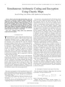
Grid Later we will subdivide [0, 1) into PN (P and N are natural numbers) semi intervals of equal length. Each has length P-N and can be identified by its left edge. These left edge points form a grid G(PN). Coordinate of a point of the grid with index k is evidently kP-N. We will use notation gk(N) for points from G(PN).

Picture 1. Grid P2 (P=2) These indexes will play an important role in our discussion. If fact, all calculations will be done using indexes. The range of indexes is 0 ≤ k < PN In other words, indexes are nonnegative numbers modulo PN. Negative numbers are defined in this ring as -k = PN - k

Weight interval Following the main idea of arithmetic coding let map alphabet A to a semi interval [0, 1), which we will refer as a weight interval. To do this enumerate symbols from A in any order (the order is not important in a sense that compression rate does not depend on it) and divide the interval in |A| semi intervals. Semi interval [wi, wi+1) corresponds to symbol ai. To make compression effective lengths of these intervals must be equal to probability of symbols in a message: | wi - wi+1 | = pi where pi – probability of symbol ai.

3

4/5/2007

Picture 2. Weight interval To define weight intervals we will use notation: { symbol0:[semininterval1), … , symbol|A|-1:[semininterval|A|-1) } For example: {a:[0, 0.5), b:[0.5, 0.75), c:[0.75, 0.875), d:[0.875,1)}

Message interval Let fix a natural number N, a prime number P and create a grid G(PN). Messages will be mapped to semi intervals [l, r) of this interval. 0≤l x = m0P0 + m1P1 + m2P2+ … + mN-jPN-j where j ≥ 0

14

4/5/2007 If last j coefficient were zero, negative lifting also does not change x as an integer number. To use negative lifting without changing results we need to know an order of the last non zero coefficient: lnz(x) = min( j: mk =0 for k>j) This function gives us the highest possible for x level. A semi interval [x y) may be positioned at level hpl(x,y) = max(lnz(x), lnz(y)) Our procedure for calculating common path length of a semi interval was defined for intervals at hpl level. To extend it for the case when an interval belongs to a fixed level we need first to lift it back to hpl. comP,N( x, y ) = N if ( x == y ) else ordP(x - y) comP,N( x, y ) = comP,hpl(x,y) (lift(x, hpl(x,y) - N ), lift(y, hpl(x,y) -N ) ) Fortunately we do not have to go in that complication. The reason for this is that lifting does not change number of common paths. Let explore previous example restricting all calculations to level 4.

0

1/4

1/2

3/4

1

{} 0

{0}

{1}

1 {b} {0, 0}

{0, 1}

{1, 0}

{1, 1}

2 {b} {0, 0, 0}

{0, 0, 1}

{0, 1, 0}

{0, 1, 1}

{1, 0, 0}

{1, 0, 1}

{1, 1, 0}

{1, 1, 1}

3

{0, 0, 0, 1}

{0, 0, 1, 1}

{0, 1, 0, 1} {0, 1, 1, 1}

{1, 0, 0, 1}

{1, 0, 1, 1}

{1, 1, 0, 1}

{1, 1, 1, 1}

4 {0, 0, 0, 0}

{0, 0, 1, 0} {0, 1, 0, 0}

{0, 1, 1, 0}

{1, 0, 0, 0}

{1, 0, 1, 0}

{1, 1, 0, 0}

{1, 1, 1, 0}

After rescaling Before rescaling

Picture 7a. Rescaling on level 4 Consider two paths x and y from the previous example, but fixed the level equal to 4. On this level x and y can be presented as {0, 0, 1, 0} and {0, 1, 1, 0} or, as p-adic numbers: x = 0*20 + 0*21 + 1*22 + 0*23 = 4 y = 0*20 + 1*21 + 1*22 + 0*23= 6 To determine common path length we need to calculate y^ -1 = 5 (y^ -1)^ = 10 (y^ -1)^ - x = 6 And finally

15

4/5/2007 com2,4(x, y) = ord2(6) = 1 After rescaling we have new x and y: x = 0*20 + 1*21 + 0*22 = 2 y = 1*20 + 1*21 + 0*22 = 3 But they belong to level 3. To return x and y back to level 4 lifting is needed: lift(x, 1) = 0*20 + 1*21 + 0*22 + 0*23 lift(y, 1) = 1*20 + 1*21 + 0*22 + 0*23

Finding the shortest path point When coding is over we can choose any paths to any point from a final semi interval as a result. But points from the same semi interval may and have different paths after dropping trailing zeros. Let take a simple example when a message finally ends with semi interval [g5(4), g10(4)). Because we can drop trailing zeros, point g8(4) is the best choice – after dropping trailing zeros it becomes g1(1).

0

1/4

1/2

3/4

1

g0(0) 0

g0(1)

g1(1)

1

g0(2)

g1(2)

g2(2)

g3(2)

2

g1(3)

g0(3)

g3(3)

g2(3)

g4(3)

g5(3)

g6(3)

g7(3)

3

g1(4)

g3(4)

g5(4)

g7(4)

g9(4)

g11(4)

g13(4)

g15(4)

4 g0(4)

g2(4)

g4(4)

g6(4)

g8(4)

g10(4)

g12(4)

g14(4)

Picture 8. Shortest path point A shortest path point in a semi interval [l, r) can be defined as a point with minimum level. lv(x^) = max(i: mi ≠ 0) g = min(lv(x^): l ≤ x < r ) But let consider paths as integers. From this point of view a point with minimal path is just a minimal padic integer. So g = min(x^: l ≤ x < r) We can check this for our example: Point Path p-adic number Index

g5(4) {0, 1, 0, 1} 10 5

g6(4) {0, 1, 1, 0} 6 6

g7(4) {0, 1, 1, 1} 15 7

g8(4) {1, 0, 0, 0} 1 8

g9(4) {1, 0, 0, 1} 9 9

g10(4) {1, 0, 1, 0} 5 10

16

4/5/2007

Model Model is just an abstraction for a set of functions. One function calculates new subinterval on a base of incoming symbol and current interval in a predefined grid. M.code(a, l, r) => lnew, rnew An other takes as arguments a point and current interval and returns a new subinterval and a symbol M.decode(g, l, r ) => lnew, rnew, a l, r, g belongs to grid G(PN), a – to alphabet A. Model operates with indexes from a ring of nonnegative integers modular PN, so we have three possible variants how one subinterval on a ring can be situated inside another: 0 ≤ l ≤ lnew < rnew ≤ r < PN r=0 ; 0 ≤ l ≤ lnew < rnew < PN r=0 ; rnew = 0; 0 ≤ l ≤ lnew < PN And, of course some technical things: initialization and taking care of end of message. M.init(A, P, N, x) Where A is alphabet, P, N – characteristics of grid G(PN), x – optional parameter, some auxiliary information, which may be used by a model for optimization. code and decode functions may update model, but they must do it in sync.

Input and Output I (input) and O (Output) are abstracts for pushing and receiving information. To make notations short we introduce an ugly term P-bit, which means one of symbols 0, … P-1. For P=2 it is obviously a normal bit. Now let describe input and output operations. I.getC => returns next character from input stream or EOM (End Of Message) I.getB(n) => returns next n P-bit vector from input stream O.pushB(U ) – pushes all P-bits from vector U O.pushB(p, n) – pushes P-bit p n times O.pushC(a) – pushes a symbol to an output stream

Algorithms Now we are in position to describe the p-adic coding algorithm. Main idea of this algorithm is the same as in arithmetic coding – a message is mapped to in interval on [0, 1). There two parts of the algorithm – encoding and decoding, but whatever we are doing the first step – initialize a model: M.init(A, N)

Coding Start with an empty message – no symbols. An empty message is coded as [0, 1), empty path U = {} or as [0, 0). l, r = 0, 0 When a symbol a comes a = I.getC model calculates a new interval.

17

4/5/2007 l, r = M.code(a, l, r) Now calculate a common path length n = comP,N(l^, (r-1)^) If n > 0 we can push common path to an output O.pushB(ext (l^, n)) and do rescaling. l^, r^ = res(l^, n), res(r^, n) And we also need to lift rescaled values back to level N and convert to index representation. l, r = lift(l^, n)^, lift(r^, n)^ Now we can read a next symbol and repeat steps.

Pseudo code M.init(A, P, N) l, r = 0, 0 while ( ( a = I.getC ) != EOM ) { l, r = M.code(a, l, r) n = comP,N(l^, (r-1)^) if ( n > 0 ) { O.pushB(ext(l^, n)) l, r = lift(res(l^, n), n)^, lift(res(r^, n), n)^ } //if } //while l, r = M.code(EOM, l, r) q = selectPoint(l, r) O.pushB(ext(q, lnz(q)) We do not specify here what selectPoint does. The only requirement is to return a grid point from final semi interval [l, r), but of cause, it’s a good idea to return a point with a shortest paths. As it follows from previous discussion, all we need is to find a minimal integer in p-adic representation. So, to select a point with minimal path we should define selectPoint( l, r ) = min(x^: l ≤ x < r) lnz used here not to push trailing zeros.

Decoding Start with an empty message – no symbols. An empty message is coded as [0, 1), or as empty path U={} or as pair of indexes: l, r = 0, 0 As the first step read first N P-bits from an input stream and construct a number from the vector. We need also to transform a path we a getting from a stream, to a number, so we use operator ^. g= (I.getB(n) • PTN)^ where PTN is a vector PN = (P0, P1, P2, … , PN) Model calculates a new interval and a symbol a M.decode(g, l, r ) => l, r, a Now, a is a new decoded symbol and can be pushed into a stream of decoded symbols

18

4/5/2007 O.pushC(a) Next, as in the coding algorithm, calculate common path length n = comP,N(l^, (r-1)^) If n > 0 we can drop common path and do rescaling. l, r, g = lift(res(l^, n), n)^, lift(res(r^, n), n)^, lift(res(g^, n))^ read additional n P-bits and recalculate g g = g + (I.getB(n) • PTn)^ Now we can repeat all steps.

Pseudo code M.init(A, P, N) l, r = 0, 0 g = (I.getB(n) • PTN)^ while ( true ) { l, r, a = M.decode(g, l, r ) if ( a == EOM ) break O.pushC(a) n = comP,N(l^, (r-1)^) if ( n > 0 ) { l, r, g = lift(res(l^, n), n)^, lift(res(r^, n), n)^, lift(res(g^, n),n)^ g = g + (I.getB(n) • PTn)^ } //if } //while

One important particular case – Huffman codes Now we are prepared to show that p-adic coding algorithm gives exactly the same codes as Huffman’s algorithm [Huffman] if a weight interval is prepared in a special way. Let as assume that for a given alphabet and symbol probabilities a Huffman code tree was constructed. For example: Symbol (s): Codeword (h(s)): Grid level (cl(s)): Starting index in grid:

a 000 3 0

b 001 3 1

C 10 2 2

d 01 2 1

e 11 2 3

We can map the tree to weight interval using the same technique as we used for coding messages

19

4/5/2007

Picture 9. Mapping Huffman code tree to weight interval After lifting all intervals to highest grid (N=3): Symbol (s): Codeword (lift(h(s),N-cl(s)): Starting index in grid:

a 000 0

B 001 1

c 100 4

d 010 2

e 110 6

Algorithm of constructing weight intervals from a Huffman code tree for alphabet A is simple. Let cl(s) be a length of Huffman code of symbol s and N = max(cl(s)) among all s from A, h(s) Huffman code of s, then symbols s occupies a semi interval starting at point with index lift(h(s),N-cl(s))^ and ending at starting point of a next symbol or 1. Constructed weight interval has an important property – all of subintervals occupy a whole grid interval of some level. It was shown above that in this situation left end right ends have an entire path in common; so PR rescaling will push all of it into an output and a next symbol will be coded starting with [0,1) interval. This proves that for this particular choice of weight interval p-adic coding works identical to Huffman’s algorithm.

Another particular case – Golomb-Rice codes Surprisingly enough, but p-adic coding algorithm produces Golomb-Rice [Golomb, Rice] codes when supplied with single symbol alphabet and special model; no changes to algorithm itself are needed. If an alphabet contains only one symbol, the only information a message may contains is its length. So coding of a message is equivalent to coding of a natural number – the length. We will use symbol * to identify the only entry. The model is trivial: M.code(*, l, r) => l, r-1 M.code(EOM, l, r) => r-1, r M.decode(g, l, r ) => if (g == r-1) then l, r, EOM else l, r-1, * The algorithm will do all the work. Let start with P=2 and consider a grid 2N+1. Coding procedure starts with l=r=0

20

4/5/2007 If a message is empty, we have to encode EOM. To do this we need to calculate r-1= 0 - 1, which is 2N+1-1 and return a path to 2N+1-1. This path consists of N+1 ones: {1, 1, … , 1, 1}. This is our new representation of zero. If a symbol comes, the model recalculates r and l: l=0 r = 2N+1-1 If it was the only symbol in a message, then the model returns 2N+1-2, 2N+1-1, and a code is a path to a point with index 2N+1-2: {1, 1, … , 1, 0}. This procedure may be continued until a message’s length is less than 2N. At this point the model returns l=0 r = 2N because comP,N(0^, (2N -1)^) = 1 PR rescaling will be used; one 0 will be pushed to output buffer, l and r return to their initial values l = r = 0. The coder is in initial state and ready to receive a new symbol. Encoder stays almost without changes. We have defined selectPoint( l, r ) = l And drop lnz call in the last pushB operation to keep trailing zeros O.pushB(ext(q)) If a messages of length W comes W/2N zeros will be pushed in output buffer; the rest part of the output will contain a path to a point which index is 0 – (W%2N). After encoding EOM we have to move the point one step to the left. So finally index will be 0 – ((W%2N) + 1). For example, for N=3 we have: W 0 1 2 3 4 5 6 7

code 1111 1110 1101 1100 1011 1010 1001 1000

W 8 9 10 11 12 13 14 15

Code 01111 01110 01101 01100 01011 01010 01001 01000

The codes look very much like Golomb-Rice codes. Indeed, they may be transformed to each other by replacing 1 with 0, and 0 with 1 - binary NOT. There is no magic in changing unary representation and delimiter – there is no difference between counting a number 0 of before first 1 and counting number of 1 before first 0. Transformation of the rest part – after delimiter, may be not that clear. In the ring of integers modular 2N 0 – (R +1) = (2N - 1) - R here R = (W%2N); R < 2N. In binary representation (2N – 1) is a vector U of N 1. Now NOT(U – R) = R This proves that after NOT transformation the rightmost part of codes transforms to W%2N.

21

4/5/2007 Any prime P can be used with this model. But this generalization does not look very promising. In fact, the reason why we discuss Huffman and Golomb-Rice codes here is to emphasize that the most popular entropy codes have a common base – they all maps messages to p-adic integer numbers.

Rescaling based on Archimedean distance (AR) We were very ingenious when selecting most convenient for us weigh interval: {a:[0, 0.5), b:[0.5, 0.75), c:[0.75, 0.875), d:[0.875,1)} Yes, compression rate does not depend on an order of subintervals, but calculation and resulted codes do. Let shuffle the weigh interval: {b:[0, 0.25), a:[0.25, 0.75), c:[0.75, 0.875), d:[0.875,1)} Now subinterval a:[0.25, 0.75) covers the center point 1/2. Consider now a message containing only symbols a. It can be easily shown that left edge of message interval will be always less than 1/2, while the right one – greater. From p-adic point of view this means that ordp(l, r) is always zero and there is no common path and, as a sequence, rescaling will never happen. If we continue coding {a, a, … , a} we will end in integer overflow error or will be faced to use infinite precision arithmetic. To save our integer arithmetic from huge numbers we have to use the fact that Archimedean length in this case is less or equal to1/2.

Picture 10. Coding {a, a, a} For P ≠ 2 situation is more complex. A semi interval can include any grid point 0 < n < P. In the following example (P = 3) an interval has Archimedean length 2/9, but p-adic length 1.

22

4/5/2007

Picture 11. Before rescaling Now let explore a case when a sub interval lies in the smallest interval of level 2, which includes a point of level 1 with index n. p-adic representation of left l and right r edges of such subinterval is. l = {n-1, P-1, …. } r = {n, 0, … } It’s Archimedean length is less or equal to 2/(P*P). We want to map it to a bigger interval, precisely to interval [n-1, n+1) from level 1. This can be done by a linear transformation: Y(X) = XP1 – nP0 +nP-1 Let’s consider how a semi interval defined in p-adic representation as l = m0P0 + m1P1 + m2P2+ … + mNPN r = k0P0 + k1P1 + k2P2+ … + kNPN transforms under this mapping. The first thing we need to do – to transform paths to points. We can do it by using IP transformation: a = m0P-1 + m1P-2 + m2P-3+ … + mNP-N-1 b = k0P-1 + k1P-2 + k2P-3+ … + kNP-N-1 Now we can apply linear transformation: Y(a) = (m0 - n)P0 + (m1 + n)P-1 + m2P-2+ … + mNP-N Y(b) = (k0 - n) P0+ (k1 + n) P-1 + k2P-2+ … + kNP-N For this subinterval we have: m0 = n -1; m1 = P- 1 k0 = n; k1 = 0 So Y(a) = 0P0 + (n - 1)P-1 + m2P-2+ … + mNP-N Y(b) = 0P0+ nP-1 + k2P-2+ … + kNP-N Rescaling will drop first zero terms. Reverting back from points to paths we can find how this transformation works on paths: Y(l) = (n - 1) P0 + m2P1+ … + mnPN-1 Y( r ) = nP0 + k2P1+ … + knPN-1 Or in vector representation:

23

4/5/2007 Y(l) = {n-1, P-1, …. } => {n -1, … } Y(r) = {n, 0, … } => {n, … } we just remove second (counting from the left) elements. It is also easy to verify that center point {n, 0, 0, …, 0} of this mapping is a stable point, i.e. Y maps it to itself Y : {n, 0, 0, …, 0} => {n, 0, …, 0} New interval [l, r) contains the stable point. Coming back to the example (here n=1) we can draw the picture after rescaling:

Picture 11a. After rescaling We will refer this rescaling as AR. Important difference between AR and PR rescaling is that AR does not push anything in output buffer. It is convenient to invent a special predicate AR? for testing if AR rescaling can be applied for an interval. AR?(l, r, P) = (r[0] – l[0] == 1) AND (l[1] == P-1) AND (r[1] == 0) To continue coding we must remember the applied mapping, it can be done by storing only two parameters: n – a stable point and u – a number of times rescaling was applied. What may happen if we continue coding? 1. [l, r) are still contains n 1.1. value of AR? predicate is false 1.2. value of AR? predicate is true 2. [l, r) does not contain n 2.1. n lays to the right of r; toRight?( n, r) == true 2.2. n lays to the left of l; toLeft?( n, l) == true To test condition 2.1 and 2.2 we introduced two predicates toRight? and toLetf?. There predicates are suppose to receive a path as second argument, i.e. a number in p-adic integer number; first argument is an integer number toRight?(n, r) = ( r[0] < n ) OR ( r^ == n ) toLeft?(n, l) = l[0] ≥ n Now let discuss situations mentioned above: 1.1. This is the simplest case. We just continue coding. 1.2. Increase u: u = u +1; do AR rescaling and continue coding.

24

4/5/2007 2.1. This means that the whole interval lays in [{n-1, P-1, … , P-1}, {n, 0, … , 0}); where P-1 is added u times. Any subinterval from this interval has common path {n-1, P-1, … , P-1}, so we can now push this path into output and rescale l and r one more time removing fist digits. 2.2. This means that the whole interval lays in [{n, 0, … , 0, 1}, { n, 0, … , 0,1}); where 0 is added u times. Any subinterval from this interval has common path {n, 0, … , 0}, so we can now push this path into output and rescale l and r one more time removing fist digits. AR and PR rescaling procedures together guaranty that current coding interval will never be smaller than 2/P2-1/PN. This means that maximum value of indexes is 2PN-2-1.

Algorithms revised Coding with AR A new feature here, comparing to the first variant of p-adic encoding algorithm, is that we need to track AR transformation. To do this we introduce two new variables sp and spn. • sp – stable point of AR; it is a point of level 1 and may be represented as a positive integer (not path) 0 < sp < P. • spn – number of times AR was applied. Some additional operations should be done at final step. First of all we need to check, as in the main loop, if the final interval is situated to the left or to the right of a stable point and, if this is the case, do necessary pushing and then proceed to usual final search for minimal point. If not and spn is not zero, then we are lucky and we already have a point from level 1 and all we need to do is just to push out sp.

Pseudo code M.init(A, N) l, r = 0, 0 sp, spn = 0, 0 while ( ( a = I.getC ) != EOM ) { l, r = M.code(a, l, r) if ( spn ≠ 0 ) { if ( toLeft?(sp, l^) ) { O.pushB(sp, 1) O.pushB(0,spn) l, r = lift(res(l^, 1), 1)^, lift(res(r^, 1), 1)^ sp, spn = 0, 0 } //if if ( toRight?(sp, r^) ) { O.pushB(sp - 1, 1) O.pushB(P - 1, spn) l, r = lift(res(l^, 1), 1)^, lift(res(r^, 1), 1)^ sp, spn = 0, 0 } //if } //if // PR rescaling if ( spn == 0 ) { n = comP,N(l^, (r - 1)^) if ( n > 0 ) { O.pushB(ext(l^, n)) l, r = lift(res(l^, n), n)^, lift(res(r^, n), n)^

25

4/5/2007 } //if } //AR rescaling while ( AR?(l^, r^) ) { sp = r^[0] if sp == 0 spn = spn + 1 l, r = lift(cut(l^,1,1),1)^, lift(cut(r^,1,1),1)^ } //while } //while l, r = M.code(EOM, l, r) if ( spn ≠ 0 ) { if ( toLeft?(sp, l^) ) { O.pushB(sp, 1) O.pushB(0, spn) l, r = lift(res(l^, 1), 1)^, lift(res(r^, 1), 1)^ sp, spn = 0, 0 } //if if ( toRight?(sp, r^) ) { O.pushB(sp - 1, 1) O.pushB(P - 1, spn) l, r = lift(res(l^, 1), 1)^, lift(res(r^, 1), 1)^ sp, spn = 0, 0 } //if } //if if (spn == 0) { q = selectPoint(l, r) O.pushB(ext(q, lnz(q)) } else { O.pushB(sp, 1) // we already have point of level 1 } //if //the End

Decoding with AR AR rescaling is simpler for decoding process, because we do not care about pushing anything out and a final step is most simple – we just finish decoding. The only thing which is new is additional reading from an input stream.

Pseudo code M.init(A, N) l, r = 0, 0 spn = sp = 0 g = (I.getB(N) • PTN)^ while ( true ) { l, r, a = M.decode(g, l, r ) if ( a == EOM ) break O.pushC(a) if ( spn ≠ 0 ) { if ( toLeft?(sp, l^) OR toRight?(sp, r^) ) { l, r, g = lift(res(l^, 1), 1)^, lift(res(r^, 1), 1)^ , lift(res(g^, 1), 1)^ g = g + (I.getB(1) • PT1)^

26

4/5/2007 sp, spn = 0, 0 } //if } //if // PR rescaling n = comP,N(l^, (r-1)^) if ( n > 0 ) { l, r, g = lift(res(l^, n), n)^, lift(res(r^, n), n)^, lift(res(g^, n),n)^ g = g + (I.getB(n) • PTn)^ } //if // AR rescaling while ( AR?(l^, r^) ) { sp = r^[0] if sp == 0 spn = spn +1 l, r, g = lift(cut(l^,1,1),1)^, lift(cut(r^,1,1),1)^, lift(cut(g^,1,1),1)^ g = g + (I.getB(1) • PT1)^ } //while } //while //the End Of course, PT1 is just 1 and we can also omit ^ operator. The operation g = g + (I.getB(1) • PT1)^ can be replaced (in two places) by g = g + I.getB(1)

Implementation We have implemented all algorithms and all tests in Ruby [Ruby] – a new popular interpreted, dynamically typed, pure object-oriented, scripting language. And Ruby proved to be very helpful. We would hardly be able to try so many variants and run innumerous tests in any other language.

P=2 Now let discuss the practical case of P=2. All previous discussion remains valid – this is just a special case. This case has most important advantage – we can use real bits and binary vectors. This is extremely convenient. All algorithms remain the same. Only some small improvement can be done for AR rescaling. Because the only possible value for n is 1, there is no need to store it as spt. In case when toLeft? returns true we have to push 1 and a number of 0; if toRight? returns true we have to push 0 and a number of 1.

Arithmetic coding We can see that arithmetic coding is just a special case of p-adic coding for P=2. All conditions expressed there as arithmetic operations can be done on bit level. In fact, many practical implementations use shifts instead. Let us examine E1 condition: mHigh < g_Half where g_Half = 0x40000000 This condition means that most significant bit in binary representation of mHigh must be 0. This is also true for gLow because mLow < mHigh. Reverting to paths we can see that both gLow and gHigh have

27

4/5/2007 most significant bits in p-adic representation are equal to 0, so p-adic distance is less than 1 and PR condition is fulfilled. However, in p-adic coding algorithm PR rescaling works for mHigh equal to g_Half. It is this small difference makes p-adic coding algorithm works exactly as Huffman algorithm for certain models. Arithmetic coding in this situation does not provide optimal compression (see discussion in [Bodden]). AR rescaling is similar to E3. AR? predicate is equivalent to (g_FisrtQuater