P1.2
EVALUATION OF A TURBULENT MIXING LENGTH PARAMETERIZATION APPLIED TO THE CASE OF AN APPROACHING UPPER-TROPOSPHERIC TROUGH Douglas K. Miller and Donald L. Walters Naval Postgraduate School, Monterey, California Ann Slavin Boeing North America, Inc. Starfire Optical Range, NM
1. INTRODUCTION The challenge of simulating a realistic evolution of optical turbulence in the stable, free atmosphere, even under the conditions of a strong jet-streak, by a state-of-the-art mesoscale model has been documented by Walters and Miller (1999). In the case presented, Walters and Miller (1999) showed that a modification of the shear and buoyancy contributions to the simulated turbulent kinetic energy (TKE) using a Mellor-Yamada 2.5 parameterization (Mellor and Yamada 1974, 1982; Yamada 1975) resulted in model predictions which had more realistic TKE magnitudes when compared to radar, balloon, and wind tunnel measurements. What has yet to be investigated is the sensitivity of the modified version of the Bougeault and Lacarrere (1989) mixing length parameterization to initial conditions and to model vertical and horizontal resolution. The sensitivity of simulated TKE will be the focus of this study under the conditions of low and moderate turbulence which occurred with the approach of a cut-off low pressure system on 18 April 2000 over Albuquerque, New Mexico. The numerical experiments generating the results for this study will be defined in Section 2, the synoptic conditions and actual integrated optical turbulence measurements for the 18 April case study will be presented in Section 3, preliminary model results will be given in Section 4, and a summary of the study will be made in Section 5. 2. NUMERICAL EXPERIMENTS Each experiment uses the U.S. Navy Coupled Ocean Atmosphere Mesoscale Prediction System (COAMPS, version 2.0.15, Hodur 1997) nonhydrostatic mesoscale model for testing the *Corresponding author address: Douglas K. Miller, Department of Meteorology, Naval Postgraduate School, Monterey, CA 93943; email:
[email protected].
Figure 1: COAMPS nested grid configuration with grid spacings decreasing from 81 to 3 km in multiples of 3. sensitivity of the simulated free atmosphere TKE evolution to initial conditions and to horizontal and vertical model resolution. The COAMPS domain configuration, whose location is shown in Figure 1, consists of four nested domains ranging from 81 to 3 km grid spacing, with a grid spacing ratio of 3 between consecutive domains. The model top was prescribed to be at 20 km, although the effective model depth is reduced due to a sponge layer at the top which contains four model levels. Within each experiment, two 24-h COAMPS simulations are generated with initialization times of 0000 and 1200 UTC 18 April 2000. The simulations are generated using a “coldstart” approach, wherein the initial conditions have been computed using two-dimensional multiquadric univariate interpolation (2DMQ, Nuss and Titley 1994) blending available National Weather Service observations either with the National Center for Environmental Prediction
Table 1: Summary of Numerical Experiments where the naming convention is XYZ such that “X”, “Y”, and “Z” correspond to the first guess model type, the number of first guess model vertical levels, and the number of COAMPS vertical levels, respectively. Experiment 1st Guess 1st Guess COAMPS Name Model Lvls. Lvls. ELL ETA 12 45 NLL NOGAPS 12 45 EML ETA 23 45 NML NOGAPS 23 45 EHL ETA 39 45 ELH ETA 12 84 NLH NOGAPS 12 84 EMH ETA 23 84 NMH NOGAPS 23 84 EHH ETA 39 84 (NCEP) ETA model or with the U.S. Navy Navy Operational Global Atmospheric Prediction System (NOGAPS) model analysis fields as the analysis first guess. The upper-tropospheric COAMPS vertical resolution in some of the experiments is changed from 500 to 250 m to test the TKE evolution sensitivity to the mesoscale model vertical grid spacing. The list of numerical experiments included in this study is provided in Table 1. Experiments having 12 first guess model vertical levels have the wind, thermal, and moisture fields analysed via 2DMQ at the 50, 100, 150, 200, 250, 300, 400, 500, 700, 850, 925, and 1000 mb isobaric levels, in addition to at the surface. Experiments having 23 first guess model vertical levels have the analyses performed at 75, 350, 450, 550, 600, 650, 750, 800, 900, 950, and 975 mb, in addition to those at the 12 isobaric levels given previously. The experiments having 39 first guess model vertical levels have the 2DMQ analyses performed every 25 mb from the 50 to the 1000 mb level. Note that only the NCEP ETA model had information available on 39 vertical levels. 3. APRIL 18, 2000 CASE STUDY The synoptic pattern as derived from the NCEP ETA model analyses valid at 0000 UTC 18 April, shown in Figure 2, indicates a cut-off low pressure system located just off the coast of California. The 300 mb level analysis (Fig. 2a) indicates a jet streak located in the base of the trough having a maximum wind speed of 70 m s-1 . At the surface
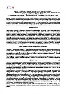
Figure 2: Analyses from the NCEP ETA model of [a] 300 mb geopotential height (m, contours) and isotachs (m s-1 , shading) and [b] mean sea level pressure (mb, contours) and 1000-500 mb thickness (m, shading) valid at 0000 UTC 18 April 2000. (Fig. 2b), the low pressure system located offshore is collocated with a dome of cold air. Another low pressure system is located further inland and eventually is associated with leeside cyclogenesis east of the Rocky Mountains. Twelve hours later, the cut-off low pressure system has propagated onshore over California and has broadened in longitudinal extent at 300 mb (Figure 3a). The corresponding jet streak has intensified slightly to a maximum speed of 74 m s-1 at 300 mb. The offshore surface low center (Figure 3b) has weakened as the system has moved toward the east. Vertical temperature and wind soundings for Albuquerque, NM valid at the same times of Figs. 2 and 3 are shown in Figure 4. Wind speeds in the 600-300 mb layer increase slightly over the 12-h period while the atmosphere from the surface to the 150 mb level has gradually cooled.
ro (cm)
Figure 4: Rawinsonde observations for Albuquerque, NM valid at [a] 0000 and [b] 1200 UTC 18 April 2000.
16 14 12 10 8 6 4 2 0 0
Figure 3: Analyses from the NCEP ETA model of [a] 300 mb geopotential height (m, contours) and isotachs (m s-1 , shading) and [b] mean sea level pressure (mb, contours) and 1000-500 mb thickness (m, shading) valid at 1200 UTC 18 April 2000. A time series of measured coherence length, ro, a parameter related to the integrated optical turbulence weighted heavily toward loweratmospheric turbulence, is shown in Figure 5 at a location just eight miles south of Albuquerque, NM. Smaller values are indicative of stronger optical turbulence. There is a diurnal component to ro, however, the plot shows a general trend with time of decreasing coherence length, implying increasingly strong optical turbulence. 4. PRELIMINARY NUMERICAL RESULTS The numerical results will focus on a comparison of experiments ELL, EML, NLL, and NML. The measured ro time series with model estimates available at 3-h intervals is shown in Figure 6. COAMPS estimates from simulations initialized using the ETA and NOGAPS models as the first
3
6
9 12 15 18 21 24 27 30 33 36
hours from 0000 UTC 18 Apr 2000
Figure 5: Observations of coherence length, ro (cm), from 0000 UTC 18 April to 1200 UTC 19 April 2000 at Starfire Optical Range. Data gap is due to the presence of clouds at the observing site. guess are indicated with a square and triangle character, respectively. Note that from 15 to 24 hours from 0000 UTC 18 April 2000, there is overlap between the simulations initialized at 0000 and at 1200 UTC 18 April, resulting in eight model data points plotted during this period. A general result is that the simulated ro values are smaller than what was observed, indicating that the predicted integrated optical turbulence was too strong. Experiments ELL and EML generally predicted stronger integrated optical turbulence than did Experiments NLL and NML. A clue for the explanation behind the systematic difference in experiments initialized with ETA or NOGAPS first guess fields is shown in Figure 7 which compares a vertical cross section for Experiment ELL (Fig. 7a) to one for Experiment
Figure 6: As in Figure 5, except with model coherence length estimates included for four experiments. NLL (Fig. 7b) which depicts wind speed, potential temperature, and Cn2, a parameter related to the optical turbulence at a given level. The simulation initialized from the ETA model shows a greater wind shear occurring within a stronger stable layer in the lower troposphere. Experiment ELL has maximum Cn2 values close to 10x10-15, whereas the maximum values corresponding to NLL reach only 6x10-15. An interesting result when intercomparing ELL to EML and NLL to NML is that the experiments show little systematic improvement between being initialized by 12 or 23 first guess model isobaric levels from hours 3 – 15. For hours 27-36, however, Experiment NML consistently gives better ro estimates than does NLL. The opposite is true for the 27-36 hour time period when comparing EML with ELL. 5. SUMMARY A series of experiments has been generated in order to examine the impact of initial conditions, and mesoscale model vertical and horizontal resolution on the simulated vertically integrated optical turbulence using a modified version of the Bougeault and Lacarrere (1989) mixing length parameterization. A case study in which a cut-off low pressure system is approaching the observation site from the west was chosen to simulate mesoscale model forecasts for 10 different experiments. Preliminary results indicate that the parameterization consistently overestimates the strength of the integrated optical turbulence. It
Figure 7: Vertical cross section depicting simulated potential temperature (K, solid contours), wind speed (m s-1, shading), and Cn2 (x1015, dashed contours) for [a] ELL and [b] NLL situated along 107o W valid at 0600 UTC 19 April 2000. should be noted, however, that the change to the mixing length parameterization is necessary to get TKE predictions to within the correct order of magnitude (Walters and Miller 1999). No single experiment clearly outperformed others when comparisons were made to ro observations, although Experiment NML (COAMPS simulation initialized from the NOGAPS first guess fields at 23 isobaric levels) showed promise later in the period as the jet streak more closely approached the observation site. The variability in the initial conditions due to the differing number of first guess isobaric model levels as well as due to differences in first guess model analyses results in the spread of the simulated ro data points plotted in Figure 6. Although the deviation between the simulated values is to within a factor of three of each other, the ensemble spread in ro does not cover the overall model bias in overestimating integrated optical turbulence. Given the location of the Cn2 maxima shown in Figure 7, it is apparent that the lower-
tropospheric TKE is being overestimated leading to unrealistically small ro values. Acknowledgements. The use of supercomputers supported by the Department of Defense High Performance Computing Modernization Program was necessary to generate the results presented in this study. 6. REFERENCES Bougeault, P. and P. Lacarrere, 1989: Parameterization of orography-induced turbulence in a mesobeta-scale model. Mon. Wea. Rev., 117, 1872-1890. Hodur, R. M., 1997: The Naval Research Laboratory’s Coupled Ocean/Atmosphere Mesoscale Prediction System (COAMPS). Mon. Wea. Rev., 125, 1414-1430. Mellor, G. L. and T. Yamada, 1974: A hierarchy of turbulence closure models for planetary boundary layers. J. Atmos. Sci., 31, 1791-1292. Mellor, G. L. and T. Yamada, 1982: Development of a turbulent closure model for geophysical fluid problems. Rev. Geophysics and Space Physics, 20, 851-875. Nuss, W. A. and D. W. Titley, 1994: Use of multiquadric interpolation for meteorological objective analysis. Mon. Wea. Rev., 122, 16111631. Walters, D. L. and D. K. Miller, 1999: Evolution of an upper-tropospheric turbulence eventcomparison of observations to numerical simulations. Preprints from the 13th Symposium on Boundary Layers and Turbulence, Dallas, Texas, 10-15 January, 157-160. Yamada, T., 1975: The critical Richardson Number and the ratio of the eddy transport coefficients obtained from a turbulent closure model. J. Atmos. Sci., 32, 926-933.