Name âColumn1â as âIDâ and assign a domain ID and number of line to skip ..... Click on calculate statistics below plane radio button and put a check mark on.
Regional Training Course on Integrated Flood Management (IFM)
Lake Tana Flood Zone Mapping Using GIS
Regional Training Course in Integrated Flood Management By Abeyou Wale Bahir Dar University, Bahir Dar Ethiopia June 07-11/2010
1
Regional Training Course on Integrated Flood Management (IFM) Part �.......................................................................................................................................................... 3 Generating Bathometric map of Lake Tana and establishing Volume-Elevation and Volume-Area curves ..................................................................................................................................................................... 3 1.1. Data format preparation (*.xls to *.csv)....................................................................................... 3 1.2. Importing bathometric data to ILWIS Environment:................................................................... 3 1.3. Table to point map........................................................................................................................ 6 1.4. Generating the surface of the lake bed / Interpolation ................................................................. 7 1.5. Opening the digital elevation mode and making profiles ............................................................ 9 1.6. Merging Bathometric data to the SRTM DEM.......................................................................... 14 1.7. Volume-Area and Volume-Elevation Relationship of Lake Tana basin.................................... 19 1.8. Fitting Volume-Elevation and Volume-Area relationship for the live storage of Lake Tana.... 25 Part �........................................................................................................................................................ 26 Areal Rainfall Estimation of Lake Tana Basin ......................................................................................... 26 2.1. Station location data format preparation “*.xls to *.csv) file format......................................... 27 2.2. Importing Rainfall station location data to ILWIS Environment:.............................................. 27 2.3. Converting attribute table to a point map................................................................................... 28 2.4. Nearest point interpolation of Metrological station ................................................................... 29 2.5. Calculating the weights of the stations....................................................................................... 32 2.6. Areal rainfall estimation............................................................................................................. 32 Part �........................................................................................................................................................ 34 Lake Tana Open water Evaporation ......................................................................................................... 34 Part �........................................................................................................................................................ 36 Runoff from rivers /inflow from rivers/.................................................................................................... 36 4.1. Runoff from gauged catchment ..................................................................................................... 36 4.2. Runoff from ungauged rivers......................................................................................................... 37 Part �........................................................................................................................................................ 38 River outflow and lake level ..................................................................................................................... 38 Part �........................................................................................................................................................ 39 Water Balance Model / Lake level simulation.......................................................................................... 39 Part �........................................................................................................................................................ 41 Flood Extent by GIS ................................................................................................................................. 41 7.1. Observing the lowest point of the basin ..................................................................................... 41 7.2. Zoning dead storage of the lake ................................................................................................. 43 7.3. Observing the extent of historical maximum flood level........................................................... 44 7.4. Flood zoning of Take Tana ........................................................................................................ 45
2
Regional Training Course on Integrated Flood Management (IFM)
Part � Generating Bathometric map of Lake Tana and establishing Volume-Elevation and Volume-Area curves 1.1.
Data format preparation (*.xls to *.csv)
o Open Bathometric data from the working directory (C:\IFM\Day5) o Click on File > Save As .. choose CSV (comma delimited in the save as type) then click on save button followed by Yes o Keep the file name as “Bathometric data”
1.2.
Importing bathometric data to ILWIS Environment:
o Opening ILWIS: go to Desktop and double click on ILWIS icon o Click on the Navigator tab under operation tree as shown below, and navigate to the working folder (C:\IFM\Day5)
3
Regional Training Course on Integrated Flood Management (IFM)
o Importing the CSV bathometric data: click on File menu > Import > Table / select “Bathometric data.csv” then click Next
o Click Next accepting the default Use ILWIS import o Click next accepting the default comma delimited type of table o You can see the attributes of the “Bathometric data” CSV file, observe that there is a label at the top of the table and it has 4 attributes ID, E, N and Lake floor altitude; click on Next button
4
Regional Training Course on Integrated Flood Management (IFM)
o The next step is Editing the table column and assigning the type of domain for the attribute � Double click on “Column1”, “Column2”,”Column3” and “Column4” and edit them as shown below � Assign the domain type for “E”, “N” and “ALT” value by double clicking on the assigned domain type � Name “Column1” as “ID” and assign a domain ID and number of line to skip will be one which is the header file finally click on Next button followed by finish
o Now after some time you will be able to see a table called “Bathometric data” under your working folder of ILWIS catalog 5
Regional Training Course on Integrated Flood Management (IFM) o Double click on the imported attribute table “Bathymetric data”; there are a total of 4660 sample points collected in and around Lake Tana.
1.3.
Table to point map
o Go to Operation menu of ILWIS main Window > Table operation > Table to point map � Select “Bathymetric data” attribute on the table list box � X column will be “E” and “N” for Y column; Coordinate system will be “UTM_m” � Write “Bath_Point” for the output point map and click on show button
6
Regional Training Course on Integrated Flood Management (IFM)
�
1.4.
The output map will show as the pattern of data collection
Generating the surface of the lake bed / Interpolation
Inverse distance weighted (IDW) interpolation determines cell values using a linearly weighted combination of a set of sample points. The weight is a function of inverse distance. By defining the higher {power} option, more emphasis can be put on the nearest points. Thus, nearby data will have the most influence, and the surface will have more detail (be less smooth). As the power increases, the interpolated values begin to approach the value of the nearest sample point. Specifying a lower value for power will provide a bit more influence to surrounding points a little farther away.
o Go to Operation tree of ILWIS main window .> Interpolation > Point interpolation > o Moving average � On the point map list box choose “Alt” on the bathymetric attribute after clicking on the plus sign � Put 2 for weighting exponent and 8000 limiting distance � Write the output name as “Bath_Raster” and use “Submap_gilgelabay” as a GeoReference from the list box (see below) � Accept the default value range and precision � Finally click on show button; after some time you will be able to see the result of the interpolation
7
Regional Training Course on Integrated Flood Management (IFM)
�
Accept the default and click ok
�
from the opened interpolated map “Bath_Raster” Click on Add layer toolbar choose “Lake” segment map: choose Black single color and line width of 3 in the display option dialog box then click on ok button. The result is shown below.
8
Regional Training Course on Integrated Flood Management (IFM) � �
1.5.
You can also Add the “Bath_Point” sample points collected, by clicking on Add layer toolbar and selecting “Bath_point” map When the Display option appears: click on symbol button and make the size to 3 to make it smaller
Opening the digital elevation mode and making profiles o Open the digital elevation model: double click on “TanaBasinDEM”; accept the default display option and click ok, click on add layer and select “Bath_Raster” with 50% Transparent under display option, add layer “Tana” segment map with Black single color and line width of 3 in the display option dialog box finally add layer “Cross section” segment map with Black single color and line width 3 in the display option dialog box o Go to File menu > open pixel information, move the pixel information dialogue box to the upper write corner of you window then, move your curser inside the lake boundary segment map and at outside the lake segment map boundary. Observe the difference from the pixel information dialogue box. o Observe; inside the lake boundary “TanaBasinDEM” measures 1786 except on the island area which is the lake level and the “Bath_Raster” reads elevation below 1786 which is the reduced level of the lake bed. What do you think the difference between those two maps “TanaBasinDEM” and “Bath_Raster” inside the lake boundary.
9
Regional Training Course on Integrated Flood Management (IFM) o Making a profile on the interpolated bathymetric map “Bath_Raster” and SRTM DEM “TanaBasinDEM” for the given “cross-section” segment map from NW to SE � Converting the line segment to a point map by distance method: go to Operation menu > vectorize > segment to point / choose the cross section segment map on segment map list box � Use the method distance put 300 m and output file name as cross section
�
Click on show button, accept the default display option and click on ok
� You can zoom in by tool bar to see the point map in detail o Extracting the elevation values of those points from the SRTM DEM “TanaBasinDEM” and interpolated Bathymetric map “Bath_Raster” � Opening the point map “cross section” as a table : right click on “cross section” point map from ILWIS catalog and click on open as table
� �
Activating the command line of the attribute: go to View menu of the attribute table and click on command line, now the command line will be visible See that there are around 225 points in the “cross section” point map and the first
10
Regional Training Course on Integrated Flood Management (IFM) attribute is Coordinate which is the X,Y location of points
MAPVALUE( ) function Returns the value, class, or ID of a map Map at a certain (X,Y) Coordinate. Syntax MAPVALUE(Map, Coordinate) Input Map is a raster, polygon, segment or point map Coordinate is an (X,Y) coordinate Domain type: a coordinate system Output MAPVALUE returns: a value, a class name or an ID Domain:
same as input Map
�
Extracting elevation value of points from SRTM DEM: write this small script on the command line of the attribute table Profile_DEM=mapvalue(TanaBasinDEM,coordinate) � Click on ok button, now a new attribute table is created with attribute name Profile_DEM: which is the Z value of the cross section points over SRTM DEM � Extracting elevation value of cross-section points on the Bath_Raster (lake bed level) model: write this small script on the command line of the attribute table Profile_BATH=mapvalue(Bath_Raster,coordinate) � Click on ok button accepting the default, now a new attribute table is created with attribute name Profile_BATH: which is the Z value of the cross section points map across the lake bed level
�
After extracting the elevation values of the point map over the two raster maps the result is shown below:
11
Regional Training Course on Integrated Flood Management (IFM)
� � � �
�
The next procedure will be plotting and observing the difference: go to Edit menu of the attribute table > select all Go to Edit menu > copy Open MS Excel: go to Start > Program files > Microsoft Excel > Microsoft Office Excel then go to edit menu and paste the coped ILWIS file Delete the first three columns which are not important to plot the profile and add a new column on the left side for the cumulative distance with 300 m interval starting from 0 distances.
Plotting the profile: go to insert menu chart of (office 2003) XY scatter chart type
12
Regional Training Course on Integrated Flood Management (IFM)
� � �
� � �
Click on Next button and click on serious tab followed by clicking add button For Serious1 give a name DEM, X value will be Distance (from 0 distance column) and Y values be Pofile_DEM column Now you will be able to see the preview
Click on Add button to add the second serious Distance VS Profile_BATH For Serious2 give a name BATH, X value will be Distance (from 0) and Y values be Pofile_BATH Click on next and enter the following information
13
Regional Training Course on Integrated Flood Management (IFM)
o Finally don’t forget to save the excel file on the working directory D:\ IFM \ day5 as “NW to SE section”. Later we will use it.
1.6.
Merging Bathometric data to the SRTM DEM
This procedure is used to merge the bathometry data into the digital elevation model at water surface (elevation of 1786) Substituting the Bath_raster data into the DEM at the water surface 14
Regional Training Course on Integrated Flood Management (IFM) IFF( ) function IFF(a, b, c) Input a Is the test condition: a boolean expression containing at least one map name or one column name. b, c expression containing at least one map name or one column name, or simply a value, class name, ID, etc. Output IFF returns: If a=true, b is returned; if a=false, c is returned; if a=undefined, undefined is returned.
Go to Operation menu > Raster operation > Map calculation : Write the following small script on the expression text box iff(TanaBasinDEM=1786,Bath_Raster, TanaBasinDEM) This script will substitute 1786 value of the DEM by the respective interpolated bathymetric data, for the values different from 1786 the digital elevation model will be kept the same o Write the output raster name as “BathDEM” and make the domain Value from the list box, see figure below:
o
o Accept the default for the value range and precision and click ok o A new map is calculated by combining the digital elevation model and the Bathometry data o Add the layer lake segment map and observe that there is no 1786 value inside the lake boundary which was the lake level, now 1786 is substituted by the lake bed level, in other words “BathDEM” is a without water map.
15
Regional Training Course on Integrated Flood Management (IFM)
Making the profile for the new “BathDEM” raster map o Opening the “cross section” point map as table: right click on Cross section point map and click on open as table � Extracting elevation value of cross-section points on the “BathDEM” (lake bed level + DEM data model): write this small script on the command line of the attribute table BathDEM=mapvalue(BathDEM,coordinate) � Click enter and accept the default values of column properties dialogue box
� � �
Click on the new attribute “BathDEM”, make a right click and copy its contents Open the saved previous excel file name “NW to SE Section” Paste the copied column and plot the BathDEM against the cumulative distance as a third series as shown below. Profile for SRTM DEM, interpolated bath and for the merged one 16
Regional Training Course on Integrated Flood Management (IFM)
Shade view of Lake Tana basin
17
Regional Training Course on Integrated Flood Management (IFM)
18
Regional Training Course on Integrated Flood Management (IFM) 1.7.
Volume-Area and Volume-Elevation Relationship of Lake Tana basin Volume-Area and Volume-Elevation relation are used for simulation of lake level, computation of Volume-Area and Volume-Elevation will be computed in ArcGIS after exporting *.asc file format o Exporting “BathDEM” ILWIS raster file to Arc/Info ASCII (.ASC) file format � Right click on “BathDEM” raster file > Slect Export.. choose Arc/Info ASCII (.ASC) form the format list box, direct the output to the working directory � Finally click on ok button
o Importing the exported “BathDEM” Asc file in to ArcGIS environment � Opening ArcGIS: go to Start > program files > ArcGIS > ArcMap finally click on ok to open a new empty map �
�
Click on add data button to add the exported ASC file format: go to the working directory select “BathDEM” and click on Add button, click on ok; ok button Double click on “BathDEM” at the table of contents: layer properties dialogue box will appear then click on Symbology followed by classified 30 classes and click on ok button
19
Regional Training Course on Integrated Flood Management (IFM)
Volume-Area and Volume-Elevation relationships can be determined using ArcGIS 3D Analyst > Surface Analyst > Area Volume Statistics Tool, the interpolated bathymetric model “BathDEM” will be sliced at 40 cm interval from the bottom of the lake 1776.2 and the respective volume, surface area and elevation will be calculated. Finally Volume-Area and Volume-Elevation relationships will be fitted by a polynomial trend to be used in the lake level simulation model. o Slicing the “BathDEM” at 40 cm interval and calculating Area, Volume and Elevation � Adding 3D Analyst toolbar: right click on any toolbar > select 3D analyst. 3D analyst toolbar will be visible on the working area � Click on the down arrow next to 3D analyst button > Surface analyst > area and volume, as shown below:
20
Regional Training Course on Integrated Flood Management (IFM)
� �
� �
Observe that minimum and maximum values of the “BathDEM” are 1772.6 and 4107.0 respectively Click on calculate statistics below plane radio button and put a check mark on save/append statistics to text file; finally show the directory for the output text file and write “Area Volume” as the file name in the working directory
Start the calculation from the lowest point 1772.6 m height of plane and click on Calculate statistics The result is shown below
21
Regional Training Course on Integrated Flood Management (IFM)
The area and volume are calculated between the reference plane and the surface. The {reference_plane} argument determines whether these calculations are performed above or below the plane. Use ABOVE or BELOW keywords to specify which option to use. When using ABOVE, the projected area and surface area for the portion of the surface above the given {base_z} are determined. The volume represents the cubic area between the plane and the underside of the surface. When using BELOW, the areas for the portion of the surface below the given {base_z} are determined. Volume is the cubic area between the plane and the top of the surface. The default {reference_plane} is ABOVE.
�
� �
Continue the calculation by entering height of the plane for 1773.0, 1773.4, 1773.8, 1774.2, 1774.6, 1775 etc up to 1791 followed by clicking Calculate statistics button; actually the historical maximum water level of the Lake Tana is 1788.02 m observed 21-Sep-1998 Finally after calculating at 40cm interval from 1772.6 to 1791.0 click on Done button Go to window explorer and open the calculation statistics “Area Volume” as text file or as excel file
22
Regional Training Course on Integrated Flood Management (IFM)
�
Elevation 1772.6 1773.0 1773.4 1773.8 1774.2 1774.6 1775.0 1775.4 1775.8 1776.2 1776.6 1777.0 1777.4 1777.8 1778.2 1778.6
After arranging the excel file the next result will be achieved
Area km2 0.00 9.05 92.01 283.91 584.78 802.39 1057.93 1228.34 1389.52 1536.12 1650.92 1757.97 1863.53 1973.88 2082.12 2174.31
Volume Mm3 0.00 0.27 18.67 97.08 270.17 540.18 904.96 1362.60 1891.18 2477.45 3112.87 3792.82 4517.29 5285.66 6097.87 6948.85
Elevation 1779.0 1779.4 1779.8 1780.2 1780.6 1781.0 1781.4 1781.8 1782.2 1782.6 1783.0 1783.4 1783.8 1784.2 1784.6 1785.0
Area km2 2258.49 2336.52 2411.97 2481.45 2551.81 2619.54 2679.81 2736.44 2789.55 2840.00 2884.95 2920.03 2950.14 2974.55 2993.75 3008.02
Volume Mm3 7834.90 8754.00 9704.14 10683.01 11688.79 12722.58 13782.16 14865.27 15970.42 17095.29 18239.57 19399.96 20573.43 21757.47 22950.03 24149.03
Elevation 1785.4 1785.8 1786.2 1786.6 1787.0 1787.4 1787.8 1788.2 1788.6 1789.0 1789.4 1789.8 1790.2 1790.6 1791.0
Area km2 3020.47 3031.37 3038.03 3043.02 3050.24 3063.99 3079.57 3116.92 3146.22 3192.79 3231.20 3265.67 3323.23 3360.74 3414.32
Volume Mm3 25354.33 26563.41 27775.99 28990.75 30208.02 31430.98 32657.52 33898.05 35145.93 36409.50 37697.00 38992.50 40316.84 41647.27 42997.56
23
Regional Training Course on Integrated Flood Management (IFM) � � �
Potting Volume-Area and Volume-Elevation by XY scatter chart type To create secondary axis, click on elevation Volume-Elevation relation and choose format data serious > Axis > click on secondary axis radio button To reverse elevation reading double click on secondary axis (elevation) > scale tab > put a check mark on values in reverse order
4000.00
1770.0 Area km2
Elevation
3500.00
2
Area (km )
2500.00
1780.0
2000.00 1785.0
1500.00 1000.00
Elevation (m amsl)
1775.0
3000.00
1790.0
500.00 0.00 0.00
10000.00
20000.00 30000.00 3 Volume (Mm )
1795.0 40000.00
Polynomial fitted Volume-Area and Volume-Elevation 3500.00
1770.0 Vol-Elev
Log. (Vol-Area)
Poly. (Vol-Elev)
1772.0 3000.00
1774.0 A = 1E-09V3 - 3E-05V2 + 0.450V + 369.9 R² = 0.975
Area (km2)
2500.00 2000.00
1776.0 1778.0 1780.0 1782.0
1500.00
1784.0 1000.00
1786.0 1788.0
500.00 0.00 0.00
E= 3E-13V3 - 2E-08V2 + 0.000V + 1773. R² = 0.995
1790.0 1792.0
7500.00
15000.00
22500.00
30000.00
37500.00
Volume (Mm3)
24
Regional Training Course on Integrated Flood Management (IFM) Lake Tana is totally controlled as long as the water level of the lake remains lower than the elevation of the spillway (1987 m amsl), the minimum operating level of the weir is 1784 m amsl. The lake level above 1784 is the live storage , Therefore we can fit this part of the lake level from 1784 up to 1789 m amsl where 1788.2 was the maximum historical lake level
1.8.
Fitting Volume-Elevation and Volume-Area relationship for the live storage of Lake Tana
o Right click on Volume-Area relationship > click on add trend > select polynomial degree 3 go to option tab and put a check mark on display equation on chart and display R-squared value on chart, repeat this procedure for the Volume-Elevation relation R2 = 0.9984 A = 1E-10*V3 - 8E-06*V2 + 0.2236*V + 853.68 E = -1E-09*V2 + 0.0004*V + 1776.2 R2 = 1
3300
Vol-Area
3200
Vol-Elev
A = 1E-10*V3 - 8E-06*V2 + 0.2236*V + 853.68 R2 = 0.9984
3100
1780 1781 1782 1783
3000
1784
2900
1785
2800
1786 1787
2700
2
E = -1E-09*V + 0.0004*V + 1776.2 R2 = 1
2600 2500 10000
15000
20000
25000
30000
1788 1789 35000
1790 40000
Volume Mm3
25
Regional Training Course on Integrated Flood Management (IFM)
Part � Areal Rainfall Estimation of Lake Tana Basin Under the working folder, there is excel file with name “rainfall data plus station location”; open and observe that there are two worksheets with name “station location” and “daily rainfall”. The nearby metrological stations around Lake Tana are Delgi, Addis Zemen, Bahir Dar, Deke Estifanos, Chawhit and Zege, there X,Y location and daily rainfall data from 1995 to 2000 is given Station location ID 1 2 3 4 5 6
Stat Name Delgi Addis Zemen Bahir Dar Deke Estifanos Chawhit Zege
X 288661.93 356387.52 325816.75 311574.51 306437.34 316875.96
Y 1351767.76 1346685.92 1282862.45 1315964.26 1363564.65 1291596.44
Daily rainfall data
Objective of the procedure � Importing the XY location of the stations in ILWIS environment as a table � Converting the table to point map � Interpolating the point map by Nearest point method /Thiesson polygon method � Masking the Thiesson polygon by Lake Tana Raster map and calculating the weights of the stations across the Lake Tana Areal rainfall.
26
Regional Training Course on Integrated Flood Management (IFM) 2.1.
Station location data format preparation “*.xls to *.csv) file format o Open “Rainfall data plus Station Location.xls” from the working directory, activate the station location worksheet o Click on File > Save As .. choose CSV (comma delimited in the save as type) and write the file name as “rainfall station location” then click on save button followed by Yes. Finally don’t forget to close the excel file, this is because file sharing is not allowed.
2.2.
Importing Rainfall station location data to ILWIS Environment: o Opening ILWIS by double clicking on desktop ILWIS icon o Click on the navigation tab under operation tree and navigate to the working folder o Importing the CSV rainfall station location data: click on File menu > Import > Table / select “rainfall station location.csv” click Next
o Click on next button, accepting the default use ILWIS import and click next accept also Comma delimited and click next see the prieview and click next o Edit the columns properties as shown below then click on next button and finally accept the default out put table name and click Finsh; as shown below
27
Regional Training Course on Integrated Flood Management (IFM)
o Now station location table is imported: double click on “rainfall station location” attribute table: the result is shown below
2.3.
Converting attribute table to a point map o Converting the attribute table to a point map: right click on “rainfall station location” attribute table > table operation > table to point map o X column will be X and Y column will be Y and use UTM_m coordinate system for the coordinate system from the list box, write the output point map as “Rainfall station”; finally click ok show button, see figure below:
28
Regional Training Course on Integrated Flood Management (IFM)
o Open the “lake” segment map and add layer “Rainfallstation” and observe the distribution of rainfall station around the lake.
2.4.
Nearest point interpolation of Metrological station o Right click on “rainfallstation” point map > interpolation > nearest point o Make submap_gilgilabay as a georeference from the list box see below. o Finally click on show button
29
Regional Training Course on Integrated Flood Management (IFM)
o Accept the default and click ok. Add “Rainfallstation” point map and “lake” segment map. Observe that all of those station will have a weight by nearest point interpolation method
o Masking “rainfallstation” thiesson polygon raster map by “Tana” raster map: go to operation main window > raster operation > map calculation o Write this small script under expression text box of map calculation dialogue box Ifnotundef(lake,rainfallstation)
30
Regional Training Course on Integrated Flood Management (IFM) IFNOTUNDEF( ) function IFNOTUNDEF(a, b) : If a is not undefined, then return b, else return undefined. IFNOTUNDEF(a, b, c): If a is not undefined, then return b, else return c.
o The result is shown below
31
Regional Training Course on Integrated Flood Management (IFM) 2.5.
Calculating the weights of the stations o Go to operation menu > statistics > histogram o Under map list box select “TanaThiess” and click on show button
o Result of the histogram ID 1 2 3 4 5 6
2.6.
Name Delgi Addis Zemen Bahir Dar Deke Estifanos Chawhit Zege
No of Pixel 54094 62517 5262 188329 40369 27579
2
Area m 438161400 506387700 42622200 1525464900 326988900 223389900
% Area 14.3 16.53 1.39 49.8 10.68 7.29
Areal rainfall estimation
Daily rainfall data for five station from Jan-1, 1992 up to Dec-31, 2000 is given o Open “Rainfall data plus Station Location.xls” from the working directory and click on “daily rainfall” worksheet o Add anew column to calculate Areal rainfall
o Areal rainfall equation for lake tana is shown below Tana Areal rainfall =0.0139*BDR + 0.143*Delgi + 0.498*Deke Estifanos + 0.1653*Addis Zemen + 0.1068*Chewhit + 0.0729 * Zege o Write the following script under Areal rainfall column in excel worksheet =0.0139*C2+0.143*D2+0.498*E2+0.1653*F2+0.1068*G2+0.0729*H2
32
Regional Training Course on Integrated Flood Management (IFM) Lake Tana daily areal rainfall
33
Regional Training Course on Integrated Flood Management (IFM)
Part � Lake Tana Open water Evaporation Evaporation is the process whereby liquid water is converted to water vapour (vaporization) and removed from the evaporating surface (vapour removal). Solar radiation, air temperature, air humidity and wind speed are climatological parameters to consider when assessing the evaporation process. For this specific study Modified penman method is used to estimate the water balance component. o
o
o o
To estimate the daily open water evaporation the nearby station Bahir Dar station is used which has a daily e maximum and minimum Temperature, average relative humidity, wind speed etc on daily basis Albedo for Lake Tana can be estimated from a number of satellite images, lake area albedo ranges from 0.05 to 0.062 an average of 0.058 is used to estimate the lake evaporation (Abeyou W. 2007)
Open the excel file under working folder with file name “Open water Evaporation” The spreadsheet has a Modified penman model used to estimate the daily open water evaporation for Bahir Dar station
The result of daily evaporation is located at AD column from 1992 to the end 2000 The result of open water evaporation shows long-term average of 1690.71 mm from 1992 to 2000 34
Regional Training Course on Integrated Flood Management (IFM)
Year 1992 1993 1994 1995 1996 1997 1998 1999 2000 Average
Total Annual Evap mm 1680.76 1677.89 1689.72 1691.37 1696.95 1709.15 1696.43 1686.01 1688.09 1690.71
35
Regional Training Course on Integrated Flood Management (IFM)
Part � Runoff from rivers /inflow from rivers/ 4.1. Runoff from gauged catchment o
o o
For this study rivers that have a continuous daily flow data recorded, only four rivers / Gigel Abay, Gumara, Ribb and Megech are used directly as an input for the water balance model to simulate lake level. The data is located in the working folder with file name “Runoff from gauged and ungauged “ under “gauged river” worksheet Total river inflow from gauged rivers is computed under Total inflow column
500 Gilgel Abay
450
Gumara
Ribb
Megech
400 350 300 250 200 150 100 50
24 -J ul -9 8
an -9 8 5J
19 -J un -9 7
ec -9 6 1D
M ay -9 6 15 -
O ct -9 5 28 -
11 -A pr -9 5
Se p94 23 -
7M
ar -9 4
0
Runoff data from gauged catchments
36
Regional Training Course on Integrated Flood Management (IFM) 4.2. Runoff from ungauged rivers An ungauged catchment is the one with inadequate records (in terms of both data quantity and quality) of hydrological observations to enable computation of hydrological variables of interest (both water quantity or quality) at the appropriate spatial and temporal scales, and to the accuracy acceptable for practical applications (PUB: Predictions in Ungauged Basins). These ungauged catchments refer to catchments having topographic and climatic properties that are available without observed discharge data. In this study runoff from ungauged catchment is adopted from Abeyou W. 2007 study, where ungauged runoff is estimated by transferring calibrated model parameters of gauged catchments based on catchment characteristics referred as regionalization. o Runoff from ungauged catchment is adopted from previous study and the result is available with file name “runoff from gauged and ungauged catchments” under the “total ungauged runoff” spreadsheet.
Runoff from ungauged
700 600 500 400 300 200 100 0 15-Jun-94
28-Oct-95
11-Mar-97
24-Jul-98
6-Dec-99
19-Apr-01
1-Sep-02
37
Regional Training Course on Integrated Flood Management (IFM)
Part � River outflow and lake level The outflow and lake level data are observed around Bahir Dar town. Outflow from Lake Tana is by the Blue Nile River which starts at Chara Chara near the city Bahir Dar. Observed lake level and out flow data are located under the working directory with file name “Lake level and outflow” o
Open the excel file in the working directory with file name “Lake level and outflow”, contains the daily lake level and outflow data from 1995 to the end 2000.
o
Figure below shows the relation between outflow by Blue Nile and the observed Lake Level Lake Level VS Outflow
800
1788.5 Outflow BN
Lake level
700
Outflow (m3/s)
600
1787.5
500 1787 400 1786.5 300 1786
200
1785.5
100 0 06/15/94
10/28/95
03/11/97
07/24/98
12/06/99
04/19/01
1785 09/01/02
Date
38
Lake level (m amsl)
1788
Regional Training Course on Integrated Flood Management (IFM)
Part � Water Balance Model / Lake level simulation After estimation of the lake water balance components (inflows such as lake areal rainfall, runoff from rivers and outflows by Blue Nile River and open water evaporation) a spreadsheet water balance model is developed to simulated lake level by volume-area and volume-elevation relationships. The initial volume and area of the lake is simply defined by fixing the initial value to an observed lake level. In the model both evaporation and rainfall are defined as a function of the lake surface area that is updated in response to the inflows and outflows. o
Opening the spreadsheet water balance model: go to the working directory and open a spreadsheet with file name “lake Tana water balance model”
o
The next step is to copy and paste the results of the water balance components from the previous excel files /Areal rainfall, open water evaporation, runoff from gauged and ungauged rivers, outflow and finally lake level to compare the result with the simulated one.
Spreadsheet model
39
Regional Training Course on Integrated Flood Management (IFM) Comparison of observed and simulated lake level
Lake Level (m amsl)
1788.5
Simulated
Observed
1787.5
1786.5
1785.5 12/7/94
12/7/95
12/6/96
12/6/97
12/6/98
12/6/99
12/5/00
Date
40
Regional Training Course on Integrated Flood Management (IFM)
Part � Flood Extent by GIS Zoneing the “BathDEM” digital elevation model:
7.1. �
Observing the lowest point of the basin
Right click on the “BathDEM” digital elevation model and choose > statistics > histogram click on Show button.
�
The minimum value is 1772.6 m amsl, to see the location of lowest point across lake Tana basin write the following script on the command line Lowest = iff(BathDEM Domain…Create new domain dialogue box will appear
45
Regional Training Course on Integrated Flood Management (IFM)
Elev 1773 1774 1775 1776 1777 1778 1779 1780 1781 1782 1783 1784 1785 1786
Upprer Bound 1773 1774 1775 1776 1777 1778 1779 1780 1781 1782 1783 1784 1785 1786
Name B1773 B1774 B1775 B1776 B1777 B1778 B1779 B1780 B1781 B1782 B1783 B1784 B1785 B1786
Code A B C D E F G H I J K L M N
Elev 1787 1788 1789 1790 1791 1792 1793 1794 1795 1796 1797 1798 1799 1800
Upprer Bound 1787 1788 1789 1790 1791 1792 1793 1794 1795 1796 1797 1798 1799 1800
Name B1787 B1788 B1789 B1790 B1791 B1792 B1793 B1794 B1795 B1796 B1797 B1798 B1799 B1800
Code O P Q R S T U V W X Y Z AA AB
o Click on ok button, Domain Group dialogue box will appear then click on Add Item button shown below;
46
Regional Training Course on Integrated Flood Management (IFM) o Then enter the upper bound, name and code starting from 1773 name B1773 and code A finally click ok
o Add also the remaining slicing zones from code B to AB by clicking on Add item button on the Domain Group dialogue box, finally the result will look like:
o Attaching the “zoning” domain to the “BathDEM” digital elevation model � Right click on the “BathDEM” digital elevation model > image processing > slicing… � Write “Flood_Zones” on the Output raster map dialogue box and choose “Zoning” Domain list box and finally click on show button.
47
Regional Training Course on Integrated Flood Management (IFM)
48
Regional Training Course on Integrated Flood Management (IFM)
49
Regional Training Course on Integrated Flood Management (IFM)
The END
50