Package LIM , implementing linear inverse models in R Karline Soetaert and Dick van oevelen Royal Netherlands Institute of Sea Research Yerseke The Netherlands
Abstract We present R package LIM (Soetaert and van Oevelen 2009) which is designed for reading and solving linear inverse models (LIM). The model problem is formulated in text files in a way that is natural and comprehensible. LIM then converts this input into the required linear equality and inequality conditions, which can be solved either by least squares or by linear programming techniques. By letting an algorithm formulate the mathematics, it becomes very simple to reformulate the model in case a parameter value changes, or a component is added or removed. Three different types of problems are supported: flow networks, reaction networks and other (operations research) problems. The first two cases are based on mass balances of the components. We give three examples, a food web example, a biogechemical reaction example and a blending example. If you use this package, please cite as: (van Oevelen, van den Meersche, Meysman, Soetaert, Middelburg, and Vezina 2009).
Keywords: Linear inverse models, flux balance analysis, linear programming, text files, R.
1. Introduction In many disciplines, mathematical formulation of problems lead to a combination of linear equalities that are supplemented with linear inequality constraints. Such linear equations arise for instance: • by considerations that certain quantities have to be positive, that the summed values should not exceed a certain value (i.e. summed fractions or probabilities should remain smaller or equal to 1), etc. • In curve fitting problems, inequality constraints may arise by requirements of monoticity, nonnegativity, convexity, while in piecewise linear fitting, equality conditions result from the need to guarantee continuity and smoothness of the curves. • In biochemical applications, the linear equalities arise because of linear conservation relationships such as the conservation of mass, charge, etc.., while inequalities ensure that
2
Package LIM , implementing linear inverse models in R mass remains a positive quantity.
2. Linear Inverse Models Mathematically, linear inverse problems can be written in matrix notation as: A·x ' b
(1)
E·x = f
(2)
G·x ≥ h
(3)
1
These are three sets of linear equations: equalities that have to be met as closely as possible (1), equalities that have to be met exactly (2) andinequalities (3). Often the problem originally only contains the latter two types of equations (2-3), and the approximate equalities are added to single out one solution. Quadratic and linear programming methods are the main mathematical techniques to solve for the vector x in this type of models. In R, these are made available through package limSolve (Soetaert, Van den Meersche, and van Oevelen 2009). Depending on the active set of equalities (2) and constraints (3), the system may either be underdetermined, even determined, or overdetermined. Solving these problems requires different mathematical techniques. • If the model is even determined, there is only one solution that satisfies the equations exactly. This solution can be singled out by matrix inversion (e.g. the solve function, in case there are no inequalities) or using the least squares method lsei from package limSolve . • If the model is overdetermined, there is only one solution in the least squares sense; this solution is singled out by function lsei (least squares with equalities and inequalities). This function also returns the parameter covariance matrix, which gives indication on the confidence interval and relationship among the estimated unknowns (elements in x). • If the model is underdetermined, there exist an infinite amount of solutions. To solve such models, there are several options: – ldei - finds the "least distance" solution, i.e. the solution with minimal sum of squared unknowns. – lsei- minimises some other set of linear functions (A · x ' b) in a least squares sense – linp - finds the solution where one linear function (i.e. the sum of unknowns) is either minimized (a "cost" function) or maximized (a "profit" function) – xranges - finds the possible ranges ([min,max]) for each unknown. 1 notations: vectors and matrices are in bold; scalars in normal font. Vectors are indicated with a small letter; matrices with capital letter.
Karline Soetaert, Dick van oevelen
3
– xsample - randomly samples the solution space using a Markov chain. This method returns the marginal probability density function for each unknown. (Van den Meersche, Soetaert, and Van Oevelen 2009) All these functions are also available from package LIM .
3. Three types of LIM One of the main remaining challenges in LIM models constitutes the setup of this type of problems. Especially when many unknowns have to be simultaneously estimated and the problem contains many equality and inequality constraints, the construction of the matrix equations may be quite complicated and error-prone. In addition to providing methods of solution, R-package LIM has been designed to facilitate problem implementation. Depending on how the problem is formulated and which are the unknowns, LIM distinguishes three types of Linear Inverse Models (Figure 1). • flow networks. Here the problem consists of a number of compartments, connected by flows. Solving the model then constitutes of deriving the values of the flows between the compartments. • reaction networks. The problem consists of a number of compartments that are involved in reactions. The LIM will estimate the reaction rates. • other. LIM can also solve problems often occurring in operational research, e.g. to find the optimal allocation of resources, optimal diet composition etc.... We give examples of these three types below.
3.1. Flow network problems Flow networks are represented as a set of nodes (compartments), which are connected by arrows (flows). The arrows generally have a direction, i.e. the flows are positive. Thus A→B denotes a flow directed from A to B, while A↔B denotes a flow that can proceed in both directions. There can only be one flow from A to B (but there can also be a flow from B to A). Solving the LIM-problem consists of finding the values of the flows. After solution, several indices and food web properties can be estimated, using functions from package NetIndices (Soetaert and Kones 2008; Kones, Soetaert, van Oevelen, and Owino 2009)
Package LIM , implementing linear inverse models in R
4
Flow network
A
J I
Reaction Network
B E
A
D
F
k2
H
B
k1
I G
C k3
F
E
D E
G
Other
C A
B p1
p2
C p3
D
Figure 1: Three types of Linear Inverse Models that can be created and solved with R package LIM . A. Flow networks. B. Reaction networks, C. Other. In type (A) and (B), a mass balance of components is generated. This is not the case for type C.
Example: a simple food-web Organisms eat and are eaten; they use part of their food for biomass production and reproduction, part is expelled as faeces or respired. Other (so-called autotrophic) organisms produce biomass from light energy and inorganic compounds, whilst dead matter (detritus) may be consumed by animals and bacteria. When the mass balances of several groups of organisms (and dead matter) are considered together, we obtain a food web model. In this type of LIM, the unknowns are the food web flows that connect the components (organisms and dead matter). Assume a simple food web comprising a plant, detritus and an animal that eats both the plant and detritus. For simplicity we assume that the system is in a climax situation, i.e. the masses, which are expressed in moles C m−2 are invariant in time. There are eight flows that connect the
Karline Soetaert, Dick van oevelen
5
components with each other and with the outside world. 2 The mass balance equation for the three components and with the rate of change = 0, is given by: dPLANT = 0 = net primary production − grazing on plant − plant mortality dt dANIMAL = 0 = grazing on plant + grazing on detritus − animal respiration dt − animal mortality − faeces production dDETRITUS = 0 = plant mortality + animal mortality + faeces production dt − grazing on detritus − detritus mineralisation These mass balances can be written in a more general way, and using shorthand notation for the flows, as: 0 = 1 · NPP − 1 · Pgraz − 1 · Pmort + 0 · Dgraz + 0 · Aresp + 0 · Amort + 0 · Faeces + 0 · Detmin (1) 0 = 0 · NPP + 1 · Pgraz + 0 · Pmort + 1 · Dgraz − 1 · Aresp − 1 · Amort − 1 · Faeces + 0 · Detmin (2) 0 = 0 · NPP + 0 · Pgraz + 1 · Pmort − 1 · Dgraz + 0 · Aresp + 1 · Amort + 1 · Faeces − 1 · Detmin (3) These equations relate, on the left hand side, the zero rates of changes to a sum of products, where each product is composed of the flows and a coefficient. The coefficient indicates if and how much these flows contribute to the rate of change. Now assume that net primary production and the total grazing rate (Grazing) of the animal has been measured (30 mmol C m−2 d −1 and 10 mmol C m−2 d −1 respectively). Thus, we can add two extra equations: NPP = 30
(4)
Pgraz + Dgraz = 10
(5)
In matrix notation, we obtain
2 Since
1 −1 −1 0 0 0 0 0 0 1 0 1 −1 −1 −1 0 0 0 1 −1 0 1 1 −1 · 1 0 0 0 0 0 0 0 0 1 0 1 0 0 0 0
NPP Pgraz Pmort Dgraz Aresp Amort Faeces Detmin
=
0 0 0 30 10
the foodweb is a subsystem of a larger system, we need to distinguish between model compartments, i.e. compartments whose dynamics are fully described in the model and external compartments, whose dynamics is coupled to processes occurring outside the model realm. The difference is essential: LIM will create mass balance equations for model compartments only. In the example, there is no balance for CO2
6
Package LIM , implementing linear inverse models in R
The feeding, defaecation and respiration flows are not independent of one another. Firstly, organisms cannot produce more faeces than the amount of food they ingest. Thus it is customary in foodweb modelling, to assume that faeces production lies in between some range of food ingested. For our example we assume that in between 30 and 60% of total food ingested is defaecated (the food is not of high quality). Secondly, organisms respire carbohydrates to provide the energy for growth. Thus, of the fraction of the food that is assimilated (i.e. not defaecated), part will be used to create new biomass, the other part will provide the energy to do so (this is referred to as the cost of growth). Here we assume that 30% of the assimilated food is respired. As total animal respiration also includes basal respiration (for the animal’s maintenance), we impose that the animal respiration has to be larger than - or equal - to this amount:
0.3 · Pgraz + 0.3 · Dgraz = Faeces
(7)
0.3 · (Pgraz + Dgraz − Faeces) = 0 0 0 0 · 0 Aresp 0 0 0 0 Amort 0 0 0 0 Faeces 1 0 0 0 Detmin 0 1 0 0 0 1
This model comprises 5 equations and 11 inequalities; there are 8 unknown flows. We will outline below how this particular problem can be implemented and solved in package LIM .
3.2. reaction problems These are LIM problems which are written as a set of reactions that connect the dynamics of several constituents. For instance, in the reaction A+B →C C is produced while A and B are consumed in a stoichiometric ratio of 1 to 1. Some reactions can occur in two directions, e.g. A+B ↔C
Karline Soetaert, Dick van oevelen
7
In contrast to previous ("flow") network problems, where only one link between two compartments was allowed, in reaction problems there may exist many links between the constituents. Solving the LIM amounts to finding values for the reaction rates.
The core metabolism of E.coli The LIM software can be used for performing flux balance analysis (e.g. (Edwards, Covert, and Palsson 2002)). See vignette ("LIMecoli") (Soetaert 2009) for an example of how to do that.
Example: chemical reactions. In the natural environment, the cycles of many constituents are linked via chemical reactions that produce and consume them. We take the biogeochemical cycling of carbon (C), nitrogen (N) and oxygen (O) in a marine sediment as an example. Organic matter ((CH2 O)106 (NH3 )16 (H3 PO4 )) is mineralized (respired), using a series of oxidants: oxygen (O2 ), nitrate (HNO3 ) and some other, undefined oxidant (XO). The reduced byproducts of this mineralization process, ammonium (NH3 ), and an undefined reduced substance (X) can be re-oxidized by a reaction with oxygen. All dissolved substances are exchanged with the water column. N2 , produced by the reaction of organic matter with nitrate, does not react in the sediment. The mineralisation reactions can be written as:
r1
(CH2 O)106 (NH3 )16 (H3 PO4 ) + 106O2 → 106CO2 + 16NH3 + H3 PO4 + 106H2 O
r2 (CH2 O)106 (NH3 )16 (H3 PO4 ) + 84.8HNO3 → 106CO2 + 42.4N2 + 16NH3 + H3 PO4 + 148.4H2 O r3
(CH2 O)106 (NH3 )16 (H3 PO4 ) + 106O2 X → 106CO2 + 106X + 16NH3 + H3 PO4 + 106H2 O
for the oxic mineralisation, denitrification and anoxic mineralisation respectively. The secondary reactions (nitrification and reoxidation of other reduced substances):
r4 r5
NH3 + 2O2 → HNO3 + H2 O X + O2 → O2 X
Package LIM , implementing linear inverse models in R
8
and the exchange with the bottom water: r6
OMBW → (CH2 O)106 (NH3 )16 (H3 PO4 )
r7
O2 ↔ O2 BW
r8
HNO3 ↔ HNO3 BW
r9
NH3 ↔ NH3 BW
r10
O2 X ↔ O2 XBW
r11
H3 PO4 ↔ H3 PO4 BW
r12
CO2 ↔ CO2 BW
Note that the deposition of organic matter (r6) is directed into the sediment, while the direction of the other fluxes can go either into or out of the sediment. In this LIM, the rates of the mineralisation reactions, of the secondary reactions and the exchange reactions with the bottom water are the unknowns (r1-r12). Based on these reactions, and following the law of conservation of mass, we can write a mass balance reaction for the following 7 constituents: (CH2 O)106 (NH3 )16 (H3 PO4 ), O2 , CO2 , NH3 , H3 PO4 , HNO3 , while for the others (e.g. O2 BW ) only part of the reactions are specified. Hence these are considered to be outside the domain of the model (externals). We give only the mass balance reactions for O2 and HNO3 : dO2 = 0 = −106 · r1 − 2 · r4 − r5 − r7 dt dHNO3 = 0 = −84.8 · r1 + ·r4 − r8 dt ··· As the exchange of dissolved substance across the sediment-water interface can go either way, directed into or out of the sediment, they can be either positive or negative. Only the rates of unidirectional reactions need be positive, and the following inequalities hold: r1 >= 0 r2 >= 0 r3 >= 0 r4 >= 0 r5 >= 0 r6 >= 0
In this particular example, the oxygen, nitrate, and ammonium fluxes have been estimated; they are -15 (influx), 1 (efflux) and 2 mmol m−2 d −1 respectively. These measurements lead to the equations:
Karline Soetaert, Dick van oevelen
9
r7 = −15 r8 = 1 r9 = 2
Thus there are 10 equations (7 mass balances, 3 measurements) and 12 unknowns. In addition, there are 6 inequality conditions3 .
3.3. other problems It is also possible to use LIM for specifying more general (linear) operational research problems that do not classify as network problems. These problems often try to find the most efficient, or least costly, way of achieving something. They are often solved with linear programming techniques that optimize some function (cost or profit) given a set of linear constraints.
blending problems This example is borrowed from limSolve and comes from the website of J E Beasley (find it on the web). A manufacturer produces a feeding mix for animals. The feed mix contains two nutritive ingredients and one ingredient (filler) to provide bulk. One kg of feed mix must contain a minimum quantity of each of four nutrients as below: Nutrient gram
A 80
B 50
C 25
D 5
The ingredients have the following nutrient values and cost: (gram/kg) Ingredient 1 Ingredient 2 Filler
A 100 200 -
B 50 150 -
C 40 10 -
D 10 -
Cost/kg 40 60 0
The problem is to find the composition of the feeding mix that minimises the production costs subject to the constraints above. Stated otherwise: what is the optimal amount of ingredients in one kg of feeding mix? 3 Note a difference with the flow networks, where the coefficients were either -1, 0, 1. Here the coefficients reflect the stoichiometry of the reaction and can differ from these numbers
10
Package LIM , implementing linear inverse models in R
Mathematically this can be estimated by solving a linear programming problem, where the equalities ensure that the sum of the three fractions equals 1, and the inequalities enforce the nutritional constraints; the quantity to be minimized is the cost function. min(x1 · 40 + x2 · 60) xi ≥ 0 x1 + x2 + x3 = 1 and 100 · x1 + 200 · x2 ≥ 80 50 · x1 + 150 · x2 ≥ 50 40 · x1 + 10 · x2 ≥ 25 10 · x1 ≥ 5
4. Specifying a Linear Inverse Model in R-package LIM The previous examples were quite simple, and the resulting matrices of small or moderate size. Nevertheless, it is easy to make mistakes. Moreover, once the matrices are constructed, it may be quite a challenge to update them after adding or removing constituents. Also, based on the resulting set of linear equations it is not straightforward to infer the underlying model assumptions. In general, a linear inverse model is first formulated verbally, after which the verbal description of the problem is translated into an equivalent mathematical description. Typically the equations are specified on aggregated unknowns, i.e. unknowns that are themselves linear combinations of other unknowns. For instance, in the food web model example, the faeces production (the flow from the animal to detritus) is specified as a part of the amount of food ingested. Ingested food is itself the sum of the flow from the plant to the animal and from detritus to the animal. Model input in LIM is close to these verbal statements. Thus to implement the food web model we first define a variable called "Ingestion" that consists of the sum of the two feeding flows and then define the defaecation constraints on this variable. When the LIM input is parsed, the constraints will be rewritten as a function of the unknowns. Apart from this more natural input, there are many other benefits of using LIM . For instance, for the flow network and reaction network type of problems, LIM generates the mass balances for each component, based on the flows or reactions that were defined. This facilitates adding or removing flows or constituents. Finally, solving the model will also generate estimates of all defined variables. We now document the input for each of the above introduced problems.
4.1. food web problem
Karline Soetaert, Dick van oevelen ===================================================== Header of the file - ignored file: foodweb.lim Solve the model in R with: require(LIM) lim Pl Pgraz : Pl -> An Pmort : Pl -> Det Dgraz : Det -> An Aresp : An ->CO2 Amort : An ->EXP Faeces: An ->Det Detmin: Det -> CO2 ## END Flows
## PARAMETERS minFaeces = 0.3 maxFaeces = 0.6 growthCost = 0.3 ## END PARAMETERS ## VARIABLES Ingestion Assimilation
= Pgraz + Dgraz = Ingestion - Faeces
11
12
Package LIM , implementing linear inverse models in R
GrowthResp = Assimilation*growthCost ## END VARIABLES ## Equalities Faeces = 30 Det -> CO2 = 10 ## End equalities ## Inequalities growthcost : Aresp > GrowthResp defaecation: Faeces = [minFaeces,maxFaeces]*Ingestion ## End inequalities
Note the use of sections (## SECTIONNAME ... ## END SECTIONNNAME) to declare items; the sections "COMPONENT" and "EXTERNAL" define the names; a mass balance equation is only generated for components, not for externals. A name is declared as "name: ", an exclamation mark ("!") demarcates the start of a comment. Although more lengthy, this problem formulation is much more elegant, more flexible, less error-prone, and easier to understand than the resulting matrices themselves. Based on this input file, the matrices are generated using LIM function Setup and put in a list (see below). The resulting LIM input can then be solved with Lsei(lim, parsimonious=TRUE) or with Ldei, which will generate the simplest -parsimonious- solution, with Xranges which will estimate ranges of unknowns, or with Xsample which will generate the conditional probability distribution of each flow. In the table below is what we obtained from running the following R-code: require(LIM) web.lim 0 r3>0 r4>0 r5>0 r6>0 ### END INEQUALITY
Results are in the following table:
r1 r2 r3 r4 r5 r6 r7 r8 r9 r10 r11 r12
min 0.00000000 0.00000000 0.06485849 1.00000000 0.00000000 0.18750000 -15.00000000 1.00000000 2.00000000 6.87500000 0.18750000 19.87500000
max 0.12264151 0.07665094 0.51709906 7.50000000 13.00000000 0.59375000 -15.00000000 1.00000000 2.00000000 54.81250000 0.59375000 62.93750000
parsimonious 0.1226364 0.00000000 0.06486363 1.00000000 0.00005450 0.18750000 -15.00000000 1.00000000 2.00000000 6.87500000 0.18750000 19.87500000
The marginal probability distribution of all reaction rates can be generated by Xsample and then simply plotted using R-function pairs. This is done in the R-script below. Before creating the pairs plot, we first remove the rates that were given a fixed value. On the diagonal of the pairs plot, we plot a histogram; we define this function first (it is copied from one of the examples in the pairs help file). We plot only the lower part of the pairs plot (i.e. set upper.panel = NULL). xs -> -> -> ->
B C C A D A
## END FLOWS ## EQUATIONS 0.5* A->B = A->C C->A = D->A C->A = f1 ## END EQUATIONS
where there are four compartments, and 6 flows. The value of the flow from C to A is specified with a parameter (f1). To solve this model, we write: Ldei("simple.input") which outputs: $X A->B A->C B->C C->A B->D D->A 1.3333333 0.6666667 0.3333333 1.0000000 1.0000000 1.0000000 $unconstrained.solution [1] 1.3333333 0.6666667 0.3333333 1.0000000 1.0000000 1.0000000 $residualNorm [1] 1.887379e-15 $solutionNorm [1] 5.333333
Package LIM , implementing linear inverse models in R
32
$IsError [1] FALSE $type [1] "ldei" Now we want solve the model successively for increasing values of the flow f1. Here is how to do this: we first create the liminput structure by just reading the input file (Read("simple.input"). This structure has a list item called "pars" which looks like: $pars name nr val par1 par2 par3 par4 var flow comp external reaction left f1 1 1 NA NA NA NA NA NA NA NA NA (it specifies the name f1 and the value (val) = 1. We then loop over all required values of f1 (for ( pars in seq(0,1,by=0.2))), each time setting the value of the parameter in the liminput structure (ls$pars$val D D->A 0.00000000 0.0 0.0 0.0 0.06666667 0.2 0.2 0.2 0.13333333 0.4 0.4 0.4 0.20000000 0.6 0.6 0.6 0.26666667 0.8 0.8 0.8 0.33333333 1.0 1.0 1.0
5
A list of all functions in LIM is in table (1). A list of useful functions in other packages is table (2) 5 For
the die-hard who has actually reached this part of the vignette. R makes a vignette only from files that have
Karline Soetaert, Dick van oevelen
33
extension "rnw" and that are then processed by R-function Sweave (Leisch 2002). Sweave interprets the R-code and makes a tex file. When I started writing, I did not yet know how to Sweave. By renaming the "tex" file as "rnw", R is tricked to believing it is a true Sweave file (which it is not) and thus makes a vignette. This means that the "R-code" that you can read is not interpreted
Package LIM , implementing linear inverse models in R
34
Table 2: Table 1. Summary of the functions in package limSolve Function Flowmatrix Plotranges PrintMat Read Setup Ldei Linp Lsei Xranges Varranges Xsample Varsample
Description Generates a flow matrix from a LIM problem Plots minimum and maximum (ranges) and a central value of a LIM problem Print the matrices of a LIM problem Reads a LIM input file and creates a liminput list Composes a LIM problem from either a liminput list or from a file Solves a LIM problem using ldei (Least distance programming with equalities and inequalities) Solves a LIM problem using Linear programming Solves a LIM problem using lsei (Least squares with equality and inequality conditions) Calculates ranges of unknowns Calculates ranges of variables (linear combinations of unknonws) Randomly samples a LIM problem for the unknowns Randomly samples a LIM problem for the inverse variables
Karline Soetaert, Dick van oevelen
35
Table 3: Table 2. Useful functions from other packages: diagram (Soetaert 2008), ToxLim (de Laender et al. 2009) and NetIndices (Soetaert and Kones 2008; Kones et al. 2009) Function
Package
Description
plotweb
diagram
plotmat
diagram
LimOmega
ToxLim
AscInd
NetIndices
Dependency
NetIndices
EffInd
NetIndices
EnvInd
NetIndices
GenInd PathInd
NetIndices NetIndices
UncInd
NetIndices
TrophInd
NetIndices
Plots a web, based on a flowmatrix 6 , thickness of arrow =value of flow Visualises the transpose of a flowmatrix 6 as labeled boxes connected by arrows (created using LIM function Flowmatrix Predicts internal concentrations of hydrophobic chemicals in aquatic organisms, based on a LIM Based on a flowmatrix 6 , estimates the ascendency network indices Based on a flowmatrix 6 , estimates the dependency network indices Based on a flowmatrix 6 , estimates the effective connectivity, flows, nodes, roles network indices Based on a flowmatrix 6 , estimates the indices of homogenization, synergism,... Based on a flowmatrix 6 , estimates the general network indices Based on a flowmatrix 6 , estimates the direct and indirecgt pathways in a network Based on a flowmatrix 6 , estimates the statistical, realised and conditional uncertainty,... Based on a flowmatrix 6 , estimates the trophic level and omnivory indices
36
Package LIM , implementing linear inverse models in R
References de Laender F, van Oevelen D, Middelburg JJ, Soetaert K (2009). “Incorporating Ecological Data and Associated Uncertainty in Bioaccumulation Modeling: Methodology Development and Case Study.” Environmental Science and Technology, 43 No. 7, 2620–2626. Diffendorfer J, Richards P, Dalrymple G, DeAngelis D (2001). “Applying Linear Programming to estimate fluxes in ecosystems or food webs: an example from the herpetological assemblage of the freshwater Everglades.” Ecological Modelling, 144, 99–120. Donali E, Olli K, Heiskanen AS, Andersen T (1999). “Carbon flow patterns in the planktonic food web of the Gulf of Riga, the Baltic Sea: a reconstruction by the inverse method.” Journal of Marine Systems, 23, 251–268. Edwards J, Covert M, Palsson B (2002). “Metabolic Modeling of Microbes: the Flux Balance Approach.” Environmental Microbiology, 4(3), 133–140. Eldridge P, Jackson G (1993). “Benthic trophic dynamics in California coastal basin and continental slope communities inferred using inverse analysis.” Marine Ecology Progress Series, 99, 115–135. Kones JK, Soetaert K, van Oevelen D, Owino J (2009). “Are network indices robust indicators of food web functioning? a Monte Carlo approach.” Ecological Modelling, 220, 370–382. doi:http://dx.doi.org/10.1016/j.ecolmodel.2008.10.012. Leguerrier D, Niquil N, Boileau N, Rzeznik J, Sauriau P, Le Moine O, Bacher C (2003). “Numerical analysis of the food web of an intertidal mudflat ecosystem on the Atlantic coast of France.” Marine Ecology Progress Series, 246, 17–37. Leisch F (2002). “Sweave: Dynamic Generation of Statistical Reports Using Literate Data Analysis.” In W Härdle, B Rönz (eds.), Compstat 2002 - Proceedings in Computational Statistics, pp. 575–580. Physica Verlag, Heidelberg. ISBN 3-7908-1517-9, URL http:// www.stat.uni-muenchen.de/~leisch/Sweave. Niquil N, Jackson G, Legendre L, Delesalle B (1998). “Inverse model analysis of the planktonic food web of Takapoto Atoll (French Polynesia).” Marine Ecology Progress Series, 165, 17– 29. Soetaert K (2008). diagram: Functions for visualising simple graphs (networks), plotting flow diagrams. R package version 1.4. Soetaert K (2009). Escherichia coli Core Metabolism Model in LIM. LIM package vignette. Soetaert K, Kones JK (2008). NetIndices: Estimating network indices, including trophic structure of foodwebs in R. R package version 1.2. Soetaert K, Van den Meersche K, van Oevelen D (2009). limSolve: Solving linear inverse models. R package version 1.5.
Karline Soetaert, Dick van oevelen
37
Soetaert K, van Oevelen D (2009). LIM: Linear Inverse Model examples and solution methods. R package version 1.4. Van den Meersche K, Soetaert K, Van Oevelen D (2009). “xsample(): An R Function for Sampling Linear Inverse Problems.” Journal of Statistical Software, Code Snippets, 30(1), 1–15. URL http://www.jstatsoft.org/v30/c01/. Van Oevelen D, Soetaert K, Middelburg J, Herman P, Moodley L, Hamels I, Moens T, Heip C (2006). “Carbon flows through a benthic food web: Integrating biomass, isotope and tracer data.” Journal of Marine Research, 64, 1–30. van Oevelen D, van den Meersche K, Meysman F, Soetaert K, Middelburg JJ, Vezina AF (2009). “Quantifying Food Web Flows Using Linear Inverse Models.” Ecosystems. doi:10.1007/s10021-009-9297-6. URL http://www.springerlink.com/content/ 4q6h4011511731m5/fulltext.pdf. Vanderbei R (2000). Linear programming, Foundations and extensions. Kluwer Academic Publishers.
Affiliation: Karline Soetaert Royal Netherlands Institute of Sea Research (NIOZ) 4401 NT Yerseke, Netherlands E-mail:
[email protected] URL: http://www.nioz.nl Dick van Oevelen Royal Netherlands Institute of Sea Research (NIOZ) 4401 NT Yerseke, Netherlands E-mail:
[email protected] URL: http://www.nioz.nl