We use the routing table at Mae-west taken on March. 15, 2002 from [12] as a base for constructing a classifier. C. Each rule in the classifier contains two fields: ...
Packet Classification Using Independent Sets Xuehong Sun and Yiqiang Q. Zhao School of Mathematics and Statistics Carleton University 1125 Colonel By Drive Ottawa, Ontario, Canada K1S 5B6 E-mail: xsun, zhao�@math.carleton.ca Abstract This paper describes a new algorithm for packet classification using the concept of independent sets. The algorithm has very small memory requirements. The search speed is neither sensitive to the size of the rule table nor to the percentage of wildcards in the fields. It also scales well from two dimensional classifiers to high dimensional ones. In particular, the algorithm is inherently parallel. Hardware tailored to this algorithm can achieve very fast search speed.
1. Introduction Internet service provider (ISP) is going to provide more value added services to end users. In order to provide these services, the router needs to classify the packets into flows according to different criteria. These criteria form rules which are based on L2/L3/L4 fields in the packet header. This function of router is called packet classification. High speed internet relies on high speed packet classification functions. In the near future, 40 Gigabit per second (OC768) wire speed is expecting to be achieved. Given the smallest packet size of 40 bytes (worst-case), the router needs to lookup packets at a speed of 125 million packets per second. That, together with other needs in processing, amounts to less than 8ns per packet lookup. Nowadays, one access to on-chip memory takes 1-5ns for SRAM and 10ns for DRAM; One access to off-chip memory takes 10-20ns for SRAM and 60-100ns for DRAM . This figure shows that it is highly demanding to develop high speed packet classification algorithms. It also shows that it is very difficult for serial algorithms to achieve ideal wire speed. Developing parallel algorithms and integrating parallel or pipeline mechanism into hardware seem a must for the future packet classification.
We propose a new algorithm using the concept of independent sets. The new algorithm is theoretically sound. Experimental studies have shown that its performance is at least comparable to best available algorithms. Specifically, the algorithm could convert a higher dimensional classification problem into a lower dimensional one. Thus, the lower bound that a dimensional classification problem requires to perform at least one-dimensional range searches is expected to break. The algorithm has very small memory requirements. The memory factor is expected to be smaller than two (The memory factor is the ratio of the total amount of memory used to that needed to store the rules). This factor was best reported in existing algorithms as four [2]. The search speed of our algorithm is neither sensitive to the size of the rule table nor the percentage of wildcards in the fields. It scales well from two dimensional classifiers to high dimensional ones. In particular, the algorithm is inherently parallel. It is easy to exploit the parallel mechanism in the hardware. One of the possible limitations of the new algorithm is that it depends on the characteristics in the rule table. Experiments show that the memory access times can be as low as 15 and as high as 100 for two-dimensional classification problems with a table size of 30000 (assuming that one dimensional range search uses four memory accesses). The rest of the paper is organized as follows. In Section 2, the packet classification problem is defined and the related notation is developed. The concept of independent sets and the details of the new algorithm are described in Section 3. In Section 4, results of experimental studies are presented. In Section 5, results from some existing algorithms are highlighted. Concluding remarks are made in Section 6.
2. Packet Classification Problem In the packet classification application, packets are classified into flows according to policy or routing information. The policy is specified using fields in the header of a packet.
Proceedings of the Eighth IEEE International Symposium on Computers and Communication (ISCC’03) 1530-1346/03 $17.00 © 2003 IEEE
Specifications of fields are called rules. So flows are specified by rules applied to incoming packets. Each rule consists of several fields, say . A collection of rules is called a classifier. Each field is either an exact value or a prefix or a range. In fact, exact values and prefixes are special ranges. In this paper, we treat fields as arbitrary ranges. Each rule also has a priority index number. Usually, the rules in a classifier are sorted according to their priorities. This index number is necessary since a packet may match more than one rule. In this case, the rule with the highbe the classifier; or est priority index is chosen. Let �½� � � � � � �, where �� �� �� � � � � � � is a rule and � is the number of the rules in the classifier. For each ��½� � � � � � ��� �, where ��� �� �� � � � � �� rule �� , let �� is the � th field. Throughout the paper, a field or a range of integers is expressed as � � � �, which means all integers greater than or equal to and smaller than or equal to . and are called the begin point and end point of the field � respectively. For example, if the field is an IPv4 destination address, then either point is an integer between � and �¿¾ � �. �� � � � � �� When a packet is arriving, the values � � �� from the relevant � fields are extracted and expressed as ��½ � � � � � ���. We say that a rule � ��½ � � � � � �� � is matched by the packet, if � � � �� for all � �� � � � � �. Among the all matched rules, the rule with the highest priority index defines the flow that the packet belongs to. With the above definitions, a rule can be considered as a hyperrectangle in the �-demensional space. A classifier is a set of such hyperrectangles. Hyperrectangles in the classifier might be overlapped. A packet is then a point in the �demensional space. Thus, packet classification is equivalent to finding all hyperrectangles which contain the query point. This resembles the point location problem in computational geometry [1]. The difference between the packet classification and the point location problem is that hyperrectangles in the point location problem are not overlapping, while hyperrectangles in the packet classification problem may overlap. Hence, the packet classification is more complex than the point location problem. However, structures and characteristics in classifiers could be exploited to develop high performance packet classification algorithms. Such packet classification algorithms may break the performance upper bound achieved in the point location background. The algorithm to be developed in this paper serves as one of such examples.
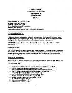
the independent sets and then explain the motivation behind the concept. �½ � � � � � � �, where �� �� Definition: Let �� � � � � � � is a rule. For index , �� � �� �, two rules �� ��½� � � � � � ��� � and �� ��½ � � � � � �� � are called independent along dimension , if � �� � ��� �. For a set � of rules, if any two rules in it are independent along dimension
, we call � an independent set along dimension , which is denoted as an �� -set or simply an � -set if no confusion arises. The number of the elements in a set � is referred to as the size of the set � denoted by ���. For a classifier, consider its all possible independent sets along dimension . An independent set with the largest size is defined as a maximum independent set along dimension in . A classifier may have more than one maximum independent set. An independent set with the largest size among all independent sets along all dimensions is called a global maximum independent set. The motivation of introducing � � -sets is that rules in an �� -set are easy to distinguish. For example, � �½ � �¾ � �¿ � as in Fig. 1 is an �½ -set in the twodimensional space. ½ � ¾ and ¿ are the begin points of field one in rules � ½ � �¾ and �¿ respectively. ½ � ¾ and ¿ define the search intervals, say � ½ � ¾ �, � ¾ � ¿ � and � ¿ � ��, in a one dimensional space. Apparently, each interval contains only one rule. Let each interval store all fields of the corresponding rule. In order to query a point, say, ��½ � �¾ �, we only need to search for the interval that �½ belongs to in one dimension. After the interval has been found, we compare the point with the rule stored in the interval. If the point is contained in the rule, there is a match. Otherwise, there is no rule matched by the point. We can easily find two advantages here. One is that we only need the begin points of the field in rules to form a range search structure instead of using both begin points and end points. This reduces the search points to as at most one half as in a traditional range search algorithm, e.g. in [2]. The other advantage is that we only need to search in one dimension rather than in all dimensions. This means
R2
3. Developing the Algorithm 3.1. Independent Sets
R3
R1
P=(f 1,f2 )
0
b1
b2
b3
Figure 1. An example of an independent set.
Our algorithm is based on the new concept of the independent sets of rules. We first give the formal definition of
Proceedings of the Eighth IEEE International Symposium on Computers and Communication (ISCC’03) 1530-1346/03 $17.00 © 2003 IEEE
that we may only need to perform one range search for a multidimensional packet classification problem. Based on the concept of independent sets, we can develop a new algorithm. The general procedure of implementing the algorithm is described as follows. Given a � � � � � � � �, we try to separate from it classifier a global maximum independent set. Then, from the set of the remaining rules (treated as a new classifier), we separate a global maximum independent set with respect to the new classifier, and continue the process until the set of the remaining rules is empty. More formally, assume that � ��� is a global maximum independent set separated from . Let � � ���, we then find a global maximum indepen� � ���, we dent set � ��� with respect to . Let � continue the process until the resulting classifier is empty. is divided into a collection of independent sets Thus, � ���� � ���� � � � � � ����. Next, we group the independent sets � ���� � ���� � � � � � ���� according to the dimension. Two independent sets belong to the same group if they are independent along the same dimension. Let � � �� � � � � � �� be the resulting groups, where � is the number of dimensions for �� � � � � �� is the group of rules in the classifier . �� �� independent sets which are independent along dimension �. Note that a group may be empty. We search in all nonempty groups of � � �� � � � � � �� respectively. The query result can be obtained by comparing all the matches to find the rule with the highest priority. In the following, we will discuss how to find a maximum independent set and how to create a data structure for search in �� �� �� � � � � ��.
Let V[] be the vertex set of the graph � � . n is the number of vertices in the graph. V[] is sorted according to the vertex degrees in increasing order. Let I be the computed maximum independent set. /*Begin Pseudocode*/ I={V[0]}; for i from 1 to n-1 if V[i] is independent of all vertices in I then I=I+{V[i]} endif endfor /*End Pseudocode*/
Figure 2. A heuristic algorithm for finding a maximum independent set in a graph.
set problem in graph theory is an NP-problem [3]. Exact algorithms are not scalable to graphs with large number of vertices. Numerous references where heuristic solutions are provided for solving this problem can be found in [4]. In our preliminary study, we choose a simple one as shown in Fig. 2 for finding a computed maximum independent set along one dimension. The intuition behind the algorithm is that the vertices of small degrees are less likely dependent of other vertices in the graph. Therefore, they have high priorities to be chosen for the testing of independence. Note that a computed maximum independent set may not be a true maximum independent set.
3.2. Finding a Global Maximum Independent Set For a classifier, there are two steps for finding a global maximum independent set. First, a maximum independent set along each dimension is found and then by comparing the size of these maximum independent sets, a global maximum independent set is identified. Finding a maximum independent set can be converted into the independent set problem in graph theory. �� � � � � ��, a graph � � corFor each dimension � responding to the independence of rules along dimension can be created as follows. A vertex in the graph � � corresponds to a rule in the classifier. There is an edge between two vertices if and only if the corresponding rules are not independent along dimension . A set of vertices is called an independent set if no pair of vertices in the set defines an edge in � � . An independent set with the maximum size is called a maximum independent set in � � . To find a maximum independent set along dimension in the classifier is equivalent to finding a maximum independent set in the graph � � . The maximum independent
3.3. Basic Data Structure for a Group of Independent Sets In this section, we develop a data structure to facilitate the search in a group of independent sets obtained from the last section. We were inspired by the fractional cascading technique [5] in developing this data structure. � ���� � ���� � � � � � ����� be a group of indeLet � pendent sets along dimension obtained in the last sec�� � � � � ��� is an independent set tion, where � � � � � and � is the number of independent sets in �. Let � � � �� � � � � � ��� �, where ��� �� �� � � � � �� � is a rule and �� is the number of rules in � � �. For each � � � � �� � � � � �� �, we extract the begin point �� of each rule ��� �� �� � � � � �� � along dimension which gives a set of points � � � � � � � �� � for each � � �. All points in
� are different, since rules in � � � are independent. We assume that all points in � are sorted in increasing order. Next, we merge the points in all � � sets � � � � � �� into a master set � . Apparently, the number of points in �
� satisfies � � � � ��� � � �, since two different sets �
Proceedings of the Eighth IEEE International Symposium on Computers and Communication (ISCC’03) 1530-1346/03 $17.00 © 2003 IEEE
�
11
3 3 b1
B3
B2
2
2
b2
b3
1
1
B1
B0
0
b1
1
1
0
b2
0
b3
B2
7
b3
0
0
b4 b5
1
b4
0
b6
1
b5
0
b7
4
6
0
B1
B0
0
may contain a same point. Let � and �. Refer to Fig. 3 for an example. The number in the rectangle (rule) is the priority of the corresponding rule. The smaller the number is, the higher the priority is. For convenience of explanation, we assume that the priority is also the index of the corresponding rule. Next, for each � �� �� � � � � �� �, we add “virtual points” to the set � . We first explain why we need the virtual points by the example in Fig. 3. The interval of ���� � ���� of � which corresponds to the interval of �� � � ��� of . There are four points � � � �� � �� and �� in the interval of ��� � �� �. Note that any rules between � � and �� and between �� and �� are dependent of rule 3; any rules between �� and �� are independent of rule 3. In order to distinguish these two situations, we add the point � � to � as a virtual point. Next, we give the definition. Let �� be the largest element in . For each ��� � � , � let �� be the end point corresponding to � �� . Let ����� � � be the successor of � �� . If the successor does not exist, let ����� �� . Assume � � � �� � such that � ��� � and � �� ���� . If there is an point � ��¼ � with � � � ��¼ � � �� such that � ��¼ is the smallest one that ��� � � ��¼ then add � ��¼ to � as a virtual point. For convenience, if the smallest � � �� � , then add �� to � as a virtual point. Each virtual point is assigned �� as its index. As in Fig. 4, the points with �� as indices are all virtual points. Our algorithm consists of two parts. One is an array that stores the classifier called the classifier array; each entry of the classifier array stores a rule which includes the fields, priority and port number. The other part is a one. Algodimensional range search structure based on rithms for one-dimensional range search are plenty in the literature. They have advantages and disadvantages. Some have small number of access memory times, while others �
��� � � � � ��
0
0
b3
b4
5
7
1
b5
2
-1
6
1
b3
-1
0
0
b4 b5
b4
0
b6
1
1
0
b7
b6
0
b8
Figure 4. A data structure example.
0
�
1
b2
2
b3
-1
12
b2
b1
b1
b8
Figure 3. Merge sets of begin points into a master set.
and
10
2
b2
1
1
1
b6
-1
9
8 2
b1
-1
3
b2
-1
2 2
b4
12
b2
b1
-1
10
5 4
B3
3 b1
9
8 2 2 b1
11
3
3 b2
b1
4
-1
-1
b2
0
4
2
-1
0 b3
1
8
-1
0 b4
-1
8
3
b5
12
-1
3
0 b6
5
10
-1
b7
0
7
9
11
0 b8
6
-1
-1
0
Figure 5. Index array pointed by leaves.
are easy to update. The multiway search [6, 7] and van Emde Boas trees [8] are among the best algorithms. The multiway search algorithm is easy to implement, but it exploits large cacheline. Van Emde Boas trees do not need a large cacheline but are complicated to implement. Here we choose the multiway search algorithm for the preliminary to create a multiway range search tree study. We use where each element in corresponds to a leaf. Each leaf points to an entry of an array which stores the indices of the � �� � � � � � � �, we find in rules as follows. For �� � � � �� � � � � � � the largest ��� such that ��� � �� . each
Each such a ��� corresponds to an index of a rule (or �� for a virtual point). There are � � indices. The indices are stored in an array pointed by the leaves. Fig. 4 and Fig. 5 illustrate an example with such a data structure. In Fig. 4, �� is the index (and priority) of a virtual point. �� has the lowest priority. Fig. 5 shows the indices array pointed by the leaves.
3.4. Search In Section 3.3., we demonstrated how to create the data structure for one group of � -set. There are at most such
Proceedings of the Eighth IEEE International Symposium on Computers and Communication (ISCC’03) 1530-1346/03 $17.00 © 2003 IEEE
data structures needed to be created. The search and update can be performed in parallel or in serial in the groups of -sets. For the search of a packet in a group, the value in the relevant field of the packet is used as the key for the search in the multiway range search tree. Find the leaf with the value that is the largest one among all which are smaller than or equal to the key. Fetch the indices pointed by the leaf. Use the indices (ignore the index ) one by one to get the rule fields by indexing into the classifier array. Compare them with the relevant fields of the packet. If there is a match, choose the matching rule with the highest priority in this group. Continue this process until all groups have been searched. Compare all the matching rules found from the groups and choose the one with the highest priority. This rule defines the flow to which the packet belongs.
3.5. Update For the dynamic packet classification, we need update the algorithm to accommodate the changes in the packet classification table. There are two kinds of updates. One is to create the table data structure from scratch whenever there is a change. Sometimes, this is called preprocessing. Another one is to modify the table data structure whenever there is a change. This is called incremental update. Usually incremental update is faster than recreating table data structure from scratch. However, incremental update may make the table data structure non optimal. Our algorithm is amenable to incremental update. Details of the update will be presented in an expanded version of this paper.
The performance of our algorithm relies on �, the number of independent sets that the classifier is partitioned into. The smaller the number is, the less memory access times and memory storage is required. Fortunately, � is not expected high. Our experimental studies and studies in the literature support this conclusion. Reference [9] observed that every packet matches at most � rules. Similar small numbers have been seen in [10]. The prefix containment is quite rare in the backbone table and is limited to at most � [9, 11]. These characteristics of classifiers guarantee that � is small. The quantitative study is provided in Section 4.
3.7. Variations So far, a basic version of the new algorithm has been described. In fact, many variations of this algorithm, which tailor to particular application or hardware architecture, could be developed. One variation is that we can increase the average search speed by sorting the indices in each entry of indices. Thus, the high priority rules are searched before the low priority rules; whenever we have a match, we will stop the search procedure. However, this change will affect the update. Another variation is that, in the index arrays, we replace the index with the corresponding rule itself. This removes the need of index access and increases the search and update speed. However, this will increase the memory storage. In the preliminary study, we use the linear search for each index in the index arrays. In fact, we can use other techniques such as a multiway search, binary search or hash search along other dimension(s) to speed up the search. We will detail the variations in our future work.
3.6. Complexities of the Algorithm
4. Experimental Study Globally, we need an array to store the classifier. The size of the array is linear to the number of rules in the classifier. In addition, a multiway range search tree will be constructed corresponding to each of at most � groups of independent sets. Assume that the group � consists of �� independent sets and contains � � rules. Then the memory storage requirement for the multiway range search tree corresponding to group � is linear to the number of � � . The number of indices stored in the leaves is at most � � � �� , since there are at most � � leaves and each leaf stores � � indices. To add all these together, the memory storage requirement for the algorithm is upper bounded by ���� �, where � is the number of rules and � is the number of total independent sets. We will see later that this bound is very loose. The memory access times consist of the times needed to search in the multiway range search trees and to fetch the indices plus � accesses to the rules.
For a classifier, we first define the repeating factor of a field. For a specified field, let � ½ be the total number of entries of the field in a classifier. Let � ¾ be the number of distinct entries of the field. The Repeating factor of the field is defined as �½ ��¾ . In the IP destination address field, the repeating factor measures the average times that an IP address is used in the rules. The performance of our algorithm is directly related to the repeating factor of each field. The data used in [2] show that repeating factors are around �� for large classifiers (with about 1M entries). The data used in [11] show that repeating factors are around � for small classifiers (with about 200 entries). For a preliminary study as in the paper, we construct classifiers with characteristics we have seen from field data. To do this, we download IP routing tables from [12] as bases and conduct several groups of experiments for two dimensional classifiers. The results are presented as follows.
Proceedings of the Eighth IEEE International Symposium on Computers and Communication (ISCC’03) 1530-1346/03 $17.00 © 2003 IEEE
4.1. Classifiers without Wildcards We first study classifiers without wildcards. In the first group of experiment, we study the effect of the repeating factor on the performance of our algorithm. In the second group we show that the size of the classifier is not sensitive to the performance of our algorithm when the repeating factor is fixed. We use the routing table at Mae-west taken on March 15, 2002 from [12] as a base for constructing a classifier . Each rule in the classifier contains two fields: The IP destination address and the source address. In the first group of experiment, we generate four classifiers of the same size of 30000 with different repeating factors. In order to generate a classifier, the expected repeating factor, say � , is given first. Then, from the Maewest routing table, ¿¼¼¼¼�� addresses are sampled. Next, from the ¿¼¼¼¼�� addresses, ¿¼¼¼¼ addresses are randomly selected as the IP destination addresses. For each destination address, the corresponding source address is randomly selected from the ¿¼¼¼¼�� addresses to form a rule. If the rule just formed is a duplicate rule of a previous generated one, we reselect a source address until the rule formed is unique. Table 1 shows the resulting classifiers. The first column is the expected repeating factor (� ). The second column is the number of distinct destination addresses (des), the third column is the repeating factor (rf) of destination address field and so on. The last column is the number of independent sets of the classifiers. We can see that the number of independent sets increases as the repeating factor increases. In the second group of experiment, six classifiers of different sizes with the same expected repeating factor of ¿¼ are constructed. The base prefixes are from the AADS routing table taken on March 15, 2002 from [12]. The results are shown in Table 2. It shows that the number of independent sets of the classifiers is not sensitive to the size of classifiers provided that the repeating factor is unchanged. This shows that our algorithm is not sensitive to the size of classifiers with a similar repeating factor. By observing data used in the literature, we found that it is rare that the
Table 1. Experiments with different repeating factors.
� 2 10 20 60
des 15422 2807 1422 489
rf 1.95 10.69 21.10 61.35
src 14321 2960 1610 498
rf 2.09 10.14 18.63 60.24
I-set 9 23 33 74
Table 2. Experiments with different table sizes. rules 2000 10000 20000 100000 200000 1000000
des 65 323 677 3499 7155 32778
rf 30.77 30.96 29.54 28.58 27.95 30.51
src 62 360 710 3287 6567 33698
rf 32.26 27.78 28.17 30.42 30.46 29.68
I-set 34 40 43 45 48 61
repeating factor exceeds 100 even for large size classifiers. Together with our experimental study, we believe that our algorithm scales well to the size of classifiers.
4.2. Classifiers with Wildcards We construct three classifiers with different percentages of wildcards in them. The base prefixes are from the AADS routing table taken on March 15, 2002 from [12]. The size of base prefixes is ¿¼¼¼¼. Given a percentage �, ��¾ percent rules have wildcards as their destination fields and ��¾ percent rules have wildcards as their source fields. Altogether, � percent rules have wildcards. The number of rules is ¿¼¼¼¼ for all three classifiers. Table 3 shows that the number of independent sets of the classifiers is not sensitive to percentage of wildcards in the classifiers. We note that the repeating factor is small and hence the number of independent sets is small. In fact, in a two-dimensional classifier, it is not possible to generate high percent wildcards in one field with a high repeating factor in the other field. We can prove the following property. Property: Assume that is a two-dimensional classifier without duplicated rules. If there are �± rules that have wildcards in one field, then the repeating factor in the other field is less than ½¼¼��. Proof: If two rules are wildcarded in one field, then the entries of these rules in the other field are distinct. Since there are �± rules that have wildcards in one field, the en-
Table 3. Experiments with different percent of wildcards. % wildcards 10 30 50
Proceedings of the Eighth IEEE International Symposium on Computers and Communication (ISCC’03) 1530-1346/03 $17.00 © 2003 IEEE
des rf 1.46 1.59 1.72
src rf 1.46 1.58 1.72
I-set 6 7 6
tries of these rules in the other field are distinct. Therefore, the number of distinct entries in the other field is of the total rules. Hence the repeating facgreater than tor in the other field is less than � .
���
��
For example, if wildcards were generated in the destination field, then the repeating factor in the source field can not be higher than two.
4.3. One Scenario of Implementation
We choose the third classifier in Table 1 for the discus� -sets for this classion of implementation. There are sifier among which are � -sets and �� -sets. Corresponding to these two groups of � -sets, two multiway range search trees are created. The multiway range search tree leaves, since corresponding to field one has at most . Each the number of distinct destination addresses is leaf points to rule indices. Since the number of rules is , each index uses bits (in fact 15 bits are enough). bytes. So the memory for the index arrays is less than Using the same argument, we find the memory for the index arrays in the other multiway range search tree is less bytes. For the array storing the rules, we asthan sume that each rule uses bits. Among the bits, bits are for begin point of the destination address field and bits for the length of the destination prefix. Another bits are for the source address field. bits are used for specbits for the port number and bits are ifying priority, empty. So rules need bytes of memory. Together, bytes memory are needed excluding for the multiway range search trees. Comparing the original rule table, our algorithm increases the memory requirement in less than a factor of one. This comes out with no surprise. On one hand, the memory requirement is large if the number of � -sets is large; on the other hand, if the number of � -sets is large, the repeating factors should be large hence the number of distinct values in a field is small, thus the number of leaves in the multiway range search tree is small. Therefore, small memory requirement is needed to store the indices array.
��
�
��
����
�
�����
��
����
� �
��
��
��
�� � ����
�� ����� � ���
����
�� �
�
The memory access times for a search depends on the bits cacheline is used. Then, cachline. We assume that memory accesses are needed for fetching the indices and memory accesses are needed for fetching the rules including port number. Excluding for the multiway range search, we need memory accesses.
�
��
� � ��
��
�
���� �����
Update is fast. Since there are only distinct source addresses, the maximum number of entries of the index arrather than . rays to be modified is
����
5. Previous Work It is difficult to make an exact comparison among all other algorithms, not only because different algorithms represent different tradeoffs, but also the databases used for experiments are different and the performance measurement is rather coarse. However, we can highlight some performance measurements for some of the algorithms. More detailed discussions on packet classification algorithms were given in [13, 14]. The Recursive Flow Classification (RFC) [15] is very fast for a search. However, the memory requirement is so large and the preprocessing time is so slow that it is not suitable for large classifiers. Reference [16] proposed a Bit Vector (BV) search algorithm. For a �-dimensional classifier, the storage requirement is � �� � , where � is the number of rules in the classifier. Query time is � times of the time needed for a range search plus � times of the time for a bit vector fetching which is equal to ���, where � is the size of cacheline. Reference [9] added new techniques to the BV algorithm and reported an order of magnitude improvement on performance over the standard BV algorithm with a small price of increasing memory requirement. The tuple space search algorithm [11] needs small memory requirement (� � ), however, the search speed depends on the number of tuples in the classifier and it supports only prefixes rather than arbitrary ranges. In addition, the use of hashing makes the time complexity of searches and updates nondeterministic [13]. The Fat Inverted Segment tree (FIS-tree) was proposed in [2]. The level of the FIS-tree can be adjusted to make a tradeoff between the search speed and memory requirements. Under the assumption that the cacheline is 32 bytes large and the entry size of a rule is 12 bytes, [2] reported that for a two dimensional classifier with more than � rules, the search needs less than 22 (17 respectively) memory accesses using three (two respectively) levels of the FIS-tree. The memory is at most � ( respectively) times of the rule table size. They did not report any experimental study on multifield classifiers. However, they pointed out that the memory requirement and memory accesses increase with a factor of � as the dimension � increases, where � is the number of levels in the FIS-tree.
��
�� �
6. Conclusions We developed a novel packet classification algorithm based on independent sets. We proposed a basic data structure and an update algorithm for the data structure. We also conducted an experimental study on our algorithm. As mentioned earlier, packet classification algorithms are measured by times of memory access, memory storage requirements, update speed and scalability, etc. Existing algorithms could perform well with respect to one or two of
Proceedings of the Eighth IEEE International Symposium on Computers and Communication (ISCC’03) 1530-1346/03 $17.00 © 2003 IEEE
these measurements. Our algorithm performs well in all aspects of the criteria. It seems that our algorithm is the first to achieve such a success: Small memory requirements, fast search and update speed and scalability to large classifier, to multidimensional classifier. The algorithm is feasible for parallel implementation. With these merits, our algorithm could be a candidate among the possible bests for the future high speed packet classification task.
7. Acknowledgments The authors would like to thank Gerard Damm and Milan Zoranovic from Alcatel for their valuable comments and suggestions. We also thank the anonymous referees for their valuable comments for revising the paper. This research is an initiative of Mathematics of Information Technology and Complex Systems, MITACS (www.mitacs.math.ca) and the National Capital Institute of Telecommunications, NCIT (www.ncit.ca) in Collaboration with Alcatel’s Research and Innovation Centre in Ottawa, Canada (www.alcatel.com).
References [1] F. Preparata and M. I. Shamos, “Computational Geometry: an Introduction,” Springer-Verlag, 1985. [2] A. Feldman and S. Muthukrishnan, “Tradeoffs for Packet Classification,” Proceedings of Infocom, v3, March 2000, pp. 1193-2002. [3] D. S. Johnson and M. A. Trick (eds.), “Cliques, Coloring, and Satisfiability: Second DIMACS Implementation Challenge,” v26, DIMACS, American Mathematical Society, 1996.
[8] D. E. Willard, “Log-logarithmic Worst-case Range Queries Are Possible in Space �� �,” Information Processing Letters, 17(2), 1983, pp. 81-84.
�
[9] Florin Baboescu and George Varghese, “Scalable Packet Classification,” ACM SIGCOMM , 2001, pp. 199-210. [10] Pankaj Gupta and Nick McKeown, “Packet Classification Using Hierarchical Intelligent Cuttings,” IEEE Micro, v20, n1, January/ February 2000, pp. 34-41. [11] V. Srinivasan, S. Suri and G. Varghese, “Packet Classification Using Tuple Space Search,” Proceedings of ACM Sigcomm, September 1999, pp. 135-146. [12] http://www.merit.edu/ipma/routing table/. [13] Pankaj Gupta and Nick McKeown, “Algorithms for Packet Classification,” IEEE Network Special Issue, March/April 2001, v15, n2, pp 24-32. [14] X. Sun, “IP Address Lookups and Packet Classification: A Tutorial and Review”, Technical Report, Carleton University, 2002. [15] Pankaj Gupta and Nick McKeown, “Packet Classification on Multiple Fields,” Proc. Sigcomm, Computer Communication Review, v29, n4, September 1999, pp. 147-160. [16] T. V. Lakshman and D. Stiliadis, “High-Speed Policy-based Packet Forwarding Using Efficient Multidimensional Range Matching,” Proceedings of ACM Sigcomm, September 1998, pp. 191-202.
[4] I. Bomze, M. Budinich, P. Pardalos and M. Pelillo, “The Maximum Clique Problem,” In D.-Z. Du and P. M. Pardalos, editors, Handbook of Combinatorial Optimization, volume 4, Kluwer Academic Publishers, Boston, MA, 1999. [5] B. Chazelle and L. J. Guibas, “Fractional Cascading I: A Data Structuring Technique,” Algorithmica , v1, n2, 1986, pp. 133-162. [6] S. Suri, G. Varghese and P.R. Warkhede, “Multiway range trees: scalable IP lookup with fast updates ”, Proc. IEEE GLOBECOM ’01 , v3 2001, pp. 1610 1614. [7] B. Lampson, V. Srinivasan and G. Varghese, “IP Lookups Using Multiway and Multicolumn Search,” Proc. IEEE INFOCOM 98 , Apr. 1998, pp. 1248-56.
Proceedings of the Eighth IEEE International Symposium on Computers and Communication (ISCC’03) 1530-1346/03 $17.00 © 2003 IEEE