Pairing Based Cryptography and Implementation in Java

Pairing Based Cryptography and Implementation in Java

Granit Luzhnica [email protected]

Institute for Applied Information Processing and Communications (IAIK) Graz University of Technology Inffeldgasse 16a 8010 Graz, Austria

Master Thesis Supervisor: Dipl.-Ing. Dr.techn. Mario Lamberger

M ay, 2011

Senat

Deutsche Fassung: Beschluss der Curricula-Kommission für Bachelor-, Master- und Diplomstudien vom 10.11.2008 Genehmigung des Senates am 1.12.2008

EIDESSTATTLICHE ERKLÄRUNG

Ich erkläre an Eides statt, dass ich die vorliegende Arbeit selbstständig verfasst, andere als die angegebenen Quellen/Hilfsmittel nicht benutzt, und die den benutzten Quellen wörtlich und inhaltlich entnommene Stellen als solche kenntlich gemacht habe.

Graz, am ……………………………

……………………………………………….. (Unterschrift)

Englische Fassung:

STATUTORY DECLARATION

I declare that I have authored this thesis independently, that I have not used other than the declared sources / resources, and that I have explicitly marked all material which has been quoted either literally or by content from the used sources.

…………………………… date

……………………………………………….. (signature)

Acknowledgements I would like to thank my supervisor Dr. Mario Lamberger for the support and guidance I received from him throughout the research needed to complete this thesis, for the effort he spent on corrections, discussions and explaining, especially in the mathematical part. Additionally, I would like to thank my family for supporting me in every step of my life.

ii

Abstract This thesis is devoted to the investigation of how bilinear pairings can be used in cryptography with a special focus on cryptographic schemes that can be build using bilinear pairings. First we describe the basic concepts of elliptic and hyperelliptic curves over finite fields, as well as rational functions and divisors on these curves. Then we introduce the Weil and Tate pairing on these curves. After that we investigate the applications of pairings in cryptography, by first investigating how pairings can be used to attack elliptic curve cryptography. Then we describe how pairings can be used to construct mathematical problems, which then serve as a basis for some interesting cryptographic schemes and protocols, which are described as well. Since the computation of a pairing is usually a costly operation, we investigate methods to optimise the pairing calculation and we provide detailed information for the most important optimisations. Finally, a pairing based cryptographic library is implemented in Java, which includes the implementation of bilinear pairings on elliptic curves, as well as the optimisations chosen from our detailed investigation. Furthermore the library provides a key agreement scheme, several encryption schemes and a signature scheme.

Keywords: elliptic curves, cryptography, public key cryptography, pairings, pairing based cryptography, PBC, identity based encryption, IBE, Bilinear Diffie-Hellman, BDH.

iii

Kurzfassung Bilineare Paarungen werden nicht mehr nur f¨ ur Angriff auf elliptischen Kurven eingesetzt, sondern k¨ onnen auch verwendet werden um einige neuartige Verschl¨ usselungsverfahren zu konstruieren, f¨ ur welche es bisher keine bekannten Konstruktionen gab. Daher ist diese Thesis der Untersuchung gewidmet, wie man bilineare Paarungen im Allgemeinen in der Kryptographie anwenden kann. In dieser Arbeit werden als erstes die grundlegenden Konzepte von elliptischen und hyperelliptischen Kurven u ¨ber endlichen Körpern beschrieben, sowie rationale Funktionen und Divisoren gefolgt von den Weil und Tate Paarungen auf diesen Kurven. Dann wird untersucht wie man Paarungen in der Kryptographie anwenden kann, z.B um Kryptographie mit elliptischen Kurven zu attackieren. Es wird beschrieben, wie Paarungen verwendet werden k¨ onnen um mathematische Probleme zu konstruieren, die als Grundlage f¨ ur einige interessante kryptographische Systeme und Protokolle dienen welche auch gut beschrieben werden. Weil die Berechnung von Paarungen in der Regel eine kostspielige Operation ist, werden Methoden zur Optimierung und dieser Berechnungen untersucht und es werden detaillierte Informationen f¨ ur die wichtigsten Optimierungen beschrieben. Schließlich wird eine Java Bibliothek f¨ ur Kryptographische Paarungen implementiert, welches die Umsetzung von bilinearen Paarungen auf elliptischen Kurven beinhaltet, sowie deren Optimierungen die aus unserer detaillierten Untersuchung hervor gegangen sind. Des Weiteren stellt die Bibliothek ein Schl¨ usselvereinbarungs-Schema, mehrere Verschl¨ usselungsverfahren und Signaturverfahren.

Stichw¨ orter: elliptische Kurven, Kryptographie, Asymmetrisches Kryptographie, Bilineare Paarungen, Kryptographische Paarungen, PBC, Identitätbasierte Verschl¨ usselung, IBE, Bilineare Diffie-Hellman, BDH.

iv

Contents 1 Introduction 2 Preliminaries 2.1 Abstract Algebra . . . . . . . . . 2.2 Elliptic Curves . . . . . . . . . . 2.2.1 Group Law . . . . . . . . 2.2.2 Elliptic Curves over Finite 2.3 Hyperelliptic curves . . . . . . . 2.3.1 Divisors . . . . . . . . . .

1

. . . . . . . . . . . . Fields . . . . . . . .

3 Pairings 3.1 The General Bilinear Pairing . . . 3.2 Weil Pairing . . . . . . . . . . . . . 3.2.1 Computing the Weil pairing 3.3 Tate Pairing . . . . . . . . . . . . . 3.3.1 Definition . . . . . . . . . . 3.3.2 Reduced Tate pairing . . . 3.3.3 Calculation . . . . . . . . . 3.4 Distortion Maps . . . . . . . . . . 3.5 Pairings on hyperelliptic curves . .

. . . . . . . . .

. . . . . . . . .

. . . . . . . . .

. . . . . .

. . . . . .

. . . . . .

. . . . . .

. . . . . .

. . . . . .

. . . . . .

. . . . . .

. . . . . .

. . . . . .

. . . . . .

. . . . . .

. . . . . .

. . . . . .

. . . . . .

. . . . . .

. . . . . .

. . . . . .

. . . . . .

. . . . . .

3 3 4 5 5 7 10

. . . . . . . . .

. . . . . . . . .

. . . . . . . . .

. . . . . . . . .

. . . . . . . . .

. . . . . . . . .

. . . . . . . . .

. . . . . . . . .

. . . . . . . . .

. . . . . . . . .

. . . . . . . . .

. . . . . . . . .

. . . . . . . . .

. . . . . . . . .

. . . . . . . . .

. . . . . . . . .

. . . . . . . . .

. . . . . . . . .

. . . . . . . . .

. . . . . . . . .

14 14 15 16 20 20 21 21 22 23

. . . . . . . . . .

24 24 25 26 27 28 29 29 30 31 32

. . . .

33 33 33 33 35

4 Public Key Cryptography 4.1 Public Key Cryptography . . . . . . . . . . . . . . . . . 4.1.1 Digital Signature . . . . . . . . . . . . . . . . . . 4.1.2 Digital Certificate . . . . . . . . . . . . . . . . . 4.2 Discrete Logarithm Problems . . . . . . . . . . . . . . . 4.3 Diffie-Hellman Protocol . . . . . . . . . . . . . . . . . . 4.4 ElGamal - DSA . . . . . . . . . . . . . . . . . . . . . . . 4.4.1 Basic ElGamal Encryption System . . . . . . . . 4.4.2 Digital Signature Algorithm - DSA . . . . . . . . 4.5 Definition of DL Problems in Pairings . . . . . . . . . . 4.6 Use of pairings to attack ECC and HECC Cryptography 5 Pairing Based Cryptography 5.1 Three party key agreement . . . . . . . . . . . . . . . 5.1.1 Three party two-round key agreement protocol 5.1.2 Three party one-round key agreement protocol 5.2 Identity Based Encryption (IBE) . . . . . . . . . . . . v

. . . .

. . . . . . . . . .

. . . .

. . . . . . . . . .

. . . .

. . . . . . . . . .

. . . .

. . . . . . . . . .

. . . .

. . . . . . . . . .

. . . .

. . . . . . . . . .

. . . .

. . . . . . . . . .

. . . .

. . . . . . . . . .

. . . .

. . . . . . . . . .

. . . .

. . . . . . . . . .

. . . .

5.3

5.4 5.5

5.2.1 Hierarchical Identity Based Encryption Scheme . . . . . . . . . . 5.2.2 Security Concepts and Definitions . . . . . . . . . . . . . . . . . 5.2.3 The Boneh-Franklin IBE Scheme . . . . . . . . . . . . . . . . . . 5.2.4 A HIBE Scheme Based on the Boneh-Frankin Scheme . . . . . . 5.2.5 The Boneh-Boyen IBE Scheme . . . . . . . . . . . . . . . . . . . 5.2.6 BB1 : Efficient IBE/HIBE From BDH Without Random Oracles 5.2.7 BB2 : Efficient IBE From BDHI Without Random Oracles . . . . Short Signatures . . . . . . . . . . . . . . . . . . . . . . . . . . . . . . . 5.3.1 Message Recovery . . . . . . . . . . . . . . . . . . . . . . . . . . 5.3.2 Security Concepts and Definitions . . . . . . . . . . . . . . . . . 5.3.3 Boneh-Lynn-Shacham (BLS) Short Signature Scheme . . . . . . 5.3.4 Boneh-Boyen short signature scheme . . . . . . . . . . . . . . . . Group signatures . . . . . . . . . . . . . . . . . . . . . . . . . . . . . . . 5.4.1 Boneh-Boyen-Shacham group signature . . . . . . . . . . . . . . Security of Pairing Based Cryptography . . . . . . . . . . . . . . . . . .

6 Implementation 6.1 Optimisations . . . . . . . . . . . . . . . . . . . . . . . . . . . 6.1.1 Pairing Optimisations . . . . . . . . . . . . . . . . . . 6.1.2 Implementation of identity based encryption (IBE and 6.1.3 Map Functions . . . . . . . . . . . . . . . . . . . . . . 6.1.4 Other Implementation Specific Optimisation . . . . . 6.2 Architecture and Design . . . . . . . . . . . . . . . . . . . . . 6.2.1 Package pairings . . . . . . . . . . . . . . . . . . . . . 6.2.2 Package crypto . . . . . . . . . . . . . . . . . . . . . . 6.2.3 Package crypto.ibe.bf . . . . . . . . . . . . . . . . . . 6.2.4 Package crypto.ibe.bb1 . . . . . . . . . . . . . . . . . . 6.2.5 Package crypto.hibe.gs . . . . . . . . . . . . . . . . . . 6.2.6 Package crypto.ssig.bls . . . . . . . . . . . . . . . . . . 6.2.7 Package crypto.tdh . . . . . . . . . . . . . . . . . . . . 6.2.8 Other Packages . . . . . . . . . . . . . . . . . . . . . . 6.3 Timing Results . . . . . . . . . . . . . . . . . . . . . . . . . . 6.3.1 Pairing calculation . . . . . . . . . . . . . . . . . . . . 6.3.2 Cryptographic operations . . . . . . . . . . . . . . . . 7 Conclusions

. . . . . . . . HIBE) . . . . . . . . . . . . . . . . . . . . . . . . . . . . . . . . . . . . . . . . . . . . . . . . . . . . . . . .

. . . . . . . . . . . . . . . . .

. . . . . . . . . . . . . . . . .

. . . . . . . . . . . . . . .

. . . . . . . . . . . . . . .

37 38 39 41 43 43 44 46 46 47 47 48 51 51 55

. . . . . . . . . . . . . . . . .

. . . . . . . . . . . . . . . . .

57 58 58 59 60 63 63 64 65 65 66 66 67 67 67 68 68 69 72

A Definitions 74 A.1 Abbreviations . . . . . . . . . . . . . . . . . . . . . . . . . . . . . . . . . . . 74 A.2 Used Symbols . . . . . . . . . . . . . . . . . . . . . . . . . . . . . . . . . . . 75 Bibliography

76

vi

Chapter 1

Introduction Since ancient times people continuously have been trying to keep information secret from others. Usually the main goal was to make some information not understandable for any one except for the parties which priory have agreed on some scheme. Nowadays, modern cryptography is present in every aspect of our life. Its job is to design cryptographic algorithms around computational hardness assumptions, such that making it infeasible for any adversary to break those algorithms. When speaking of cryptography, one should differ between symmetric key cryptography and public key cryptography. In the case of symmetric key cryptography all communicating parties share the same secret which enables them to encrypt and decrypt the information. All parties can securely communicate as long as they all possess the used secret and they are the only ones to possess it. The main practical problem with symmetric key cryptography is the distribution of the secret between parties, which is known as key exchange. When there was no public key cryptography, the key exchange was done by either physical delivery (such as face-to-face meetings, use of a trusted courier) or by sending the key through an existing encrypted channel. The problem with physical delivery is that it is very unpractical, usually expensive, mostly unsafe and one should plan communication ahead. In the case of using an existing encrypted channel the security depends on the security of a previous key exchange, because the parties should a priori have a shared secret. The solution to those problems is the is the use of public key cryptography. In public key cryptography, each entity has a public and a private key and there is no need for prior key exchange in order to securely communicate, since one makes the public key public and anyone can use it to encrypt data. Then, only the person that has the corresponding private key is able to decrypt the encrypted data. A practical problem with such public key cryptosystems is the distribution of public keys. The question is how to verify the authenticity of a public key? How to be sure that the public key really belongs to the person we think it does? Usually, in order to solve this problem, digital certificates are used. In 1985 Shamir came with another, better idea how to solve this problem. The idea was to use the identity of a user as public key (or to derive the public key directly from public key) [57]. By directly using the identity of the user as public key, the question of the public key authenticity is no longer an issue and there is no need for certificates. However, he provided only a signature scheme and for years there was no known solution for an identity based encryption scheme. Here is the point where pairings come into play. Basically, a pairing on an curve is, a function which takes two points of a specific order and outputs a element of a finite field. In 1991, Menezes, Okamoto, and Vanstone made 1

CHAPTER 1. INTRODUCTION

2

use of pairings in cryptography for the first time. They used the Weil pairing to transform the Elliptic Curve Discrete Logarithm Problem to the Discrete Logarithm Problem in a finite field, where efficient algorithms exist. In 1994, the same attack was constructed by Frey and R¨ uck using Tate pairing [22]. For years, pairings were known as good tool to constructs attacks on both, elliptic and hyperelliptic curves. This reputation changed in 2000, when Joux used pairings to construct a tripartite Diffie-Hellman key agreement protocol, by demonstrating that the pairings can be also used to construct cryptosystems rather than only for attacking purposes. Since then there have been many cryptographic schemes constructed using pairings. One of the first ones and the most popular one is the identity based encryption scheme constructed by BonehFranklin in 2001, which gave the first fully provable secure identity based encryption scheme, almost after 2 decades after the concept was introduced by Shamir. Besides the identity based encryption, there are many other applications of pairing based cryptography such as: short signatures, group signatures, etc.

Chapter 2

Preliminaries 2.1

Abstract Algebra

In this section, we will give some basic definitions and concepts of groups, rings and fields. Extended explanations can be found in [49]. Definition 2.1.1. (group). A group denoted as G is a set with some binary operation, which satisfies closure, associativity, identity and invertibility condition, also known as group axioms. The group can have a finite number of elements or an infinite number of them and this number is an important feature of the group. Definition 2.1.2. (order). The order of a group denoted as |G| is called the number of elements in G. If |G| is finite then the group is ”finite”. Definition 2.1.3. (cyclic group, generator of a group). A group G is cyclic if there is an element g ∈ G such that for each a ∈ G there is an integer i with a = g i = g · g · . . . · g . | {z } i−times

Such an element g is called a generator of G. Definition 2.1.4. (ring, commutative ting). A ring denoted R is a set with two binary operations + and · (usually called addition and multiplication), which satisfies additive associativity, additive commutativity, additive identity, additive inverse, distributivity and multiplicative associativity condition. The ring is a commutative ring if it satisfies the multiplicative commutativity condition. Finally, we come to the most important definition of this section, which is the field. Definition 2.1.5. (field). A field, denoted as F, is a commutative ring in which all non-zero elements have multiplicative inverses. F denotes the algebraic closure of F. Since the field has the closure property with some binary operation, it means that whenever we perform a binary operation, let us say addition, between two elements of the field, the result is always another element of the field. So, one can navigate through elements of the group by initially getting one element of the field and performing addition with the multiplicative identity, which results in the another element and then adding this result element again with the multiplicative identity by gaining yet another element 3

CHAPTER 2. PRELIMINARIES

4

and so on. If one keeps performing this addition and if the fields finite, then after finite n number of steps the result would be the initial element. This property (n) is called characteristic of the field. The formal definition is given below. Definition 2.1.6. (field characteristic). The characteristic of a field is the smallest number of times one must add the multiplicative identity element (1) to itself in order to gain the additive identity element (0). Example 2.1.1. Zp is a field with addition and multiplication modulo p where p is a prime. In this case the characteristic of Zp is p. Definition 2.1.7. (subfield, extension field) Let F be a field. If K is a subset of the underlying set of F which is closed with respect to the field operations and inverses in F, then K is said to be a subfield of F, and F is an extension field of K. In this case F/K (”F over K”) is said to be a field extension. Later we will deal a lot with extension fields Fq , where q = pn and p is prime. In order to represent Fpn , one finds an irreducible polynomial m(X) ∈ Fp [X] of degree n and then uses the isomorphism Fpn ' Fp [X]/(m(X)).

2.2

Elliptic Curves

In this section we will give a brief introduction to elliptic curves. The aim of this section is to introduce elliptic curves, point representation and group arithmetic of points in an elliptic curve. Most of the concepts you see in this section are taken from [31]. Definition 2.2.1. (elliptic curve over field). An elliptic curve E over the field F is described as a smooth curve in the so called long Weierstrass form: Y 2 + a1 XY + a3 Y = X 3 + a2 X 2 + a4 X + a6

(2.1)

where a1 , a2 , a3 , a4 , a6 ∈ F. The elliptic curve E(F) is the set of points (x, y) ∈ F × F that satisfy this equation, along with the point at infinity, which is denoted by O (sometimes simply by ∞). We use the expression ’the elliptic curve E over the field F’, since the coefficients ai (for 1 ≤ i ≤ 6) that are used to define the equation, are elements of the field F. The definition also states that the curve should be smooth. In order for a curve to be smooth, it must not have any singular points, which means that there must not exist a point of E(F) where both partial derivatives vanish. So, for any point P (x, y) ∈ E(F) the conditions: a1 y − 3x2 − 2a2 x − a4 = 0

(2.2)

2y + a1 x + a3 = 0

(2.3)

and must not be satisfied simultaneously.


5

This could be easily achieved by ensuring that ∆ 6= 0, where ∆ is the discriminant of E, which is defined as follows: ∆ = −d22 d8 − 8d34 − 27d26 + 9d2 d4 d6 d2 = a21 + 4a2 d4 = 2a4 + a1 a3 d6 = a23 + 4a6 d8 = a21 a6 + 4a2 a6 − a1 a3 a4 + a2 a23 − a24

2.2.1

Group Law

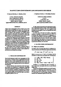
The most interesting part of elliptic curves is that the points of an elliptic curve form an abelian additive group where the addition is performed using the chord and tangent rule and O is used as identity element. In the following theorem [33, Theorem 5.5] we will give the group properties of points of the elliptic curve. Theorem 2.2.1. Let E be an elliptic curve. Then the addition law on E has the following properties: • Identity: P +O =O+P ∀ P ∈E • Inverse element: P + (−P ) = O ∀ P ∈ E • Associativity: P + (Q + R) = (P + Q) + R ∀ P, Q, R ∈ E • Commutativity: P + Q = Q + P ∀ P, Q ∈ E The chord and tangent rule is explained geometrically. For any given two points P = (x1 , y2 ) and Q = (x2 , y2 ) of an elliptic curve, in order to add them, first one should draw a straight line through P and Q. Based on the Bezout’s theorem, this line always intersects the curve at a third point R which represents −(P + Q). In order to get P + Q we need to obtain −R, which is the third intersection point of the line through R and O. If P = Q then the line through P and Q represents the tangent to the curve at P . This line intersects at the second point R. By reflecting the point R across x-axes we get −R = P + Q = P + P = 2P , which represents the double of P (see Figure 2.1).

2.2.2

Elliptic Curves over Finite Fields

We defined earlier the Elliptic curve over a field given in long Weierstrass form. Here we will define the elliptic curve over finite fields Fq = Fpn with p > 3. The equation which it is used to describe the elliptic curves in these fields gets simplified and it is called short Weierstrass form.


6

(a) Point addition P + Q = R

(b) Point doubling P + P = R

Figure 2.1: Geometric addition and doubling of elliptic curve (y 2 = x3 − x + 2) points Definition 2.2.2. (elliptic curve over finite fields). An elliptic curve E over the finite field Fpn with p > 3 is given through an equation of the form: Y 2 = X 3 + aX + b where a, b ∈ Fq and − (4a3 + 27b2 ) 6= 0. Definition 2.2.3. (supersingular curves). An elliptic curve E defined over a finite field Fq of characteristic p is supersingular if t|p, where t = q + 1 − #E(Fq ). Otherwise the curve is ordinary. The chord-tangent rule for point addition can be also used for finite fields. In fact using geometry one can derive the explicit formulas for adding and doubling points. So, let E be a elliptic curve defined over a finite field Fq and let P (x1 , y1 ), Q(x2 , y2 ) and R(x3 , y3 ) be three points of the curve E. In Table 2.1 the explicit formulas for inversion, addition and doubling of points P, Q and R in Fq are given. Table 2.1: Explicit formulas for point inversion, addition and doubling in Fq R = (−P ) R=P +Q R = 2P

x3 = x1 y3 = −y1 1 2 x3 = ( xy22 −y −x1 ) − x1 − x2 1 y3 = ( xy22 −y −x1 )(x1 − x3 ) − y1

y3 = Note that here

a b

means a · b−1 in Fq .

3x21 +a 2 2y1 ) − 2x1 3x21 +a ( 2y1 )(x1 − x3 )

x3 = (

− y1


7

The following example will show the point addition, using the formulas in table 2.1, for the elliptic curve defined over prime finite filed. Example 2.2.1. Let us pick an elliptic curve y 2 = x3 − x + 2 and a prime finite field F7 . First we need to make sure that the discriminant is not zero. −(4a3 + 27b2 ) = −(4(−1)3 + 27 · 22 ) = −(−4 + 108) = = −104 = −104 mod (7) = 1 6= 0 Here we pick a random point P = (2, 1). Now we compute point Q(x2 , y2 ) where Q = 2P . 3 · 22 − 1 2 3x21 + a 2 11 ) − 2x1 = ( ) − 2 · 2 = ( )2 − 4 = 2y1 2·1 2 −1 2 2 = (11 · 2 ) − 4 = (11 · 4) − 4 = 1932 mod (7) = 0

x2 = (

11 3 · 22 − 1 3x21 + a )(2 − 0) − 1 = ( ) · 2 − 1 = )(x1 − x3 ) − y1 = ( 2y1 2·1 2 −1 = (11 · 2 ) · 2 − 1 = 11 · 4 · 2 − 1 = 87 mod (7) = 3

y2 = (

So, now we have point Q = (0, 3) which is the double of point P = (2, 1). Now, let us try to add P and Q. So R = (x3 , y3 ) = P + Q, which means x1 = 2, y1 = 1, x2 = 0 and y2 = 3 y2 − y1 2 2 3−1 2 ) − 2 − 0 = ( )2 − 2 = ) − x1 − x2 = ( x2 − x1 0−2 −2 −1 2 2 = (2 · (−2) ) − 2 = (2 · 3) − 2 = 36 − 2 = 34 mod(7) = 6

x3 = (

y2 − y1 3−1 2 )(2 − 6) − 1 = ( )(−4) − 1 = )(x1 − x3 ) − y1 = ( x2 − x1 0−2 −2 −1 (2 · (−2) )(−4) − 1 = (2 · 3)(−4) − 1 = −24 − 1 = −25 mod(7) = 3

y3 = (

This elliptic curve has 9 points (including O), which are: P1 = (0, 3) P2 = (0, 4) P3 = (1, 3) P4 = (1, 4) P5 = (2, 1) P6 = (2, 6) P7 = (6, 3) P8 = (6, 4) P9 = O

2.3

Hyperelliptic curves

This section will give information about mathematical aspects of hyperelliptic curves (see [20, 48, 41]). In the previous section we introduced some concepts of elliptic curves, which in fact are a special class of algebraic curves. Now we will introduce the hyperelliptic curves, which are another special class of algebraic curves and can be considered as generalisation of elliptic curves.


8

An important feature is the genus of the curve which is determined from the degree of the polynomial of the curve. A polynomial of degree 2g + 1 or 2g + 2 gives a curve of genus g. There do exit hyperelliptic curves of every genus g ≥ 1. An elliptic curve represents a hyperelliptic curve of genus g = 1. Definition 2.3.1. (hyperelliptic curve) A hyperelliptic curve C of genus g (g ≥ 1) defined over F is given by equation fC : y 2 + h(x)y = f (x)

(2.4)

where h(x) ∈ F is a polynomial of degree at most g, f (x) ∈ F is a monic polynomial of degree 2g + 1 and there are no solutions (u, v) ∈ F × F which simultaneously satisfy the equation v 2 + h(u)v = f (u) and partial derivative equations 2v + h(u) = 0 and h0 (u)v − f 0 (u) = 0. A point of the elliptic curve is any solution (x, y) ∈ F × F that satisfies the Equation (2.4). The set of points is denoted by C. The set of F - rational points of the curve is denoted by C(F). Similar to the elliptic curves there exists the point of infinity denoted by O. A singular point on C is a point P = (x, x) ∈ F × F, in which the equation y 2 + h(x)v = f (x) and partial derivative equations 2y + h(x) = 0 and h0 (x)y − f 0 (x) = 0 are simultaneously satisfied. From the definition of a hyperelliptic curve and the definition of a singular point, it is easy to see that hyperelliptic curves have no singular points. For some P = (x, y) ∈ C, the opposite point is the point P˜ = (x, −y − h(x)) ∈ C. The ˜ = O). opposite point of the point at infinity is defined to be the point at infinity itself (O Finite points that satisfy (P˜ = P ) are called special points. Points that are not special, are called ordinary points. Example 2.3.1. Consider the hyperelliptic curve C given by equation: y 2 + x2 y = x5 − 4x3 + 3x over R. It is easy to see that h(x) = x2 , f (x) = x5 − 4x3 + 3x and g = 2. The plot is displayed in Figure 2.2. Example 2.3.2. Now consider the same curve used in Example 2.3.1 (y 2 + x2 y = x5 − 4x3 + 3x), but now over the finite field Z11 . We can find the Z11 -rational points that lie on the curve: P1 = (0, 0) P2 = (1, 0) P3 = (1, 10) P4 = (5, 0) P5 = (5, 8) P6 = (6, 0) P7 = (6, 8) P8 = (8, 1) P9 = (9, 1) P10 = (9, 6) P11 = (10, 0) P12 = (10, 10) P13 = O The points P1 and P11 are special points. In the case of elliptic curves we could build a group by adding points, where addition is meant to be the reflection over x-axis of the third point which is intersected, when drawing a line through two points that are being added. We cannot build a group by applying chord-and tangent rule in a hyperelliptic curve, since the line through two given points can intersect at more than a point (other than these two given points). Fortunately there is another way of building a group, by using so called divisors. Before we continue to explain the divisors we need to give some definitions regarding polynomial functions and some other related concepts.


9

Figure 2.2: Hypereliptic curve (y 2 + x2 y = x5 − 4x3 + 3x) over R Definition 2.3.2. (coordinate ring, polynomial function). The coordinate ring of C over Fq , denoted Fq [C] is the quotient ring Fq [C] = Fq [x, y]/(y 2 + h(x)y − f (x)) where (y 2 + h(x)y − f (x)) := {p(x, y) · (y 2 + h(x)y − f (x)) : p(x, y) ∈ Fq [x, y]}. This definition can be extended to Fq . An element of Fq [C] is called polynomial function on C. For each polynomial function G(x, y) ∈ Fq [C], each occurrence of y 2 can be replaced by f (x) − h(x)y, in order to get the representation G(x, y) = a(x) − b(x)y where a(x), b(x) ∈ Fq [x] and G(x, y) is unique. Definition 2.3.3. (conjugate). Let G(x, y) = a(x) − b(x)y be a polynomial function in Fq [C]. The conjugate of G(x, y) is defined to be the polynomial function G(x, y) = a(x) + b(x)(h(x) + y). Definition 2.3.4. (norm). Let G(x, y) = a(x)−b(x)y be a polynomial function in Fq [C]. The norm of G(x, y) is the polynomial function N (G) = GG. The norm of a function G(x, y) has these properties: 1. N (G) is a polynomial in Fq [x] 2. N (G) = N (G)


10

3. N (GH) = N (G)N (H) Proofs for these properties can be found at [48]. Definition 2.3.5. (function field, rational functions). The function field Fq (C) of C over Fq is the field of fractions of Fq [C]. This definition is valid also for Fq . In the case of Fq , the elements of Fq are called rational functions of C. Definition 2.3.6. (degree of a polynomial function). Let G(x, y) = a(x) − b(x)y be a non-zero polynomial function in Fq [C]. The degree of G is defined to be deg(G) = max[2degx (a), 2g + 1 + 2degx (b)] Definition 2.3.7. (order) Let G = a(x) − b(x)y ∈ Fq [C] be a non-zero polynomial function and let P = (u, v) ∈ C. The order of G at P , denoted as ordP (G), is defined as follows: 1. If P = (u, v) is a finite point, then let r be the highest power of (x − u) that divides both a(x) and b(x). In this case we can write G(x, y) = (x − u)r (a0 (x) − b0 (x)y). • If (a0 (u) − b0 (u)y) 6= 0 let s = 0 • Otherwise, let s be the highest power of (x−u) that divides N (a0 (x)−b0 (x)y) = a22 + a0 b0 h − b20 f . • If P is an ordinary point, then define: ordP (G) = r + s • If P is a special point, then define: ordP (G) = 2r + s 2. If P = O then define: ordP (G) = −max[2degx (a), 2g + 1 + 2degx (b)] Definition 2.3.8. (zero, pole). Let G ∈ Fq [C]∗ and let P = (u, v) ∈ C. If G(P ) = 0 the G is said to have a zero at P . If G is not defined at P then G is said to have a pole at P , denoted as G(P ) = ∞. Definition 2.3.9. (number of zerosPand poles). Let G ∈ Fq [C]∗ . Then G has finite number of zeros and poles. Moreover, P ∈C ordP G = 0. Proof can be found in [48].

2.3.1

Divisors

Definition 2.3.10. (divisor, degree, order). A divisor D is a formal sum of points on C X D= mP P, mP ∈ Z, P ∈C

where only a finite number of the integers mP are non-zero. The degree of D, denoted P degD, is the integer P ∈C mP . The order of D af P , denoted ordP (D), is the integer mP .


11

The set of all divisors, denoted DivC , forms an additive group under the addition rule: X X X mP P + nP P = (mP + nP )P P ∈C

P ∈C

P ∈C

0 , is a subgroup of Div . and the set of all divisors of degree 0, denoted DivC C P P Definition 2.3.11. (GCD of divisors). Let D1 = P ∈C mP P and D2 = P ∈C nP P be two divisors. The greatest common divisor of D1 and D2 is defined as X X gcd(D1 , D2 ) = min(mP , nP )P − ( min(mP , nP ))O P ∈C

P ∈C

Definition 2.3.12. (divisor of a rational function). Let R(x, y) 6= 0 ∈ Fq (C) be a rational function. The divisor of R is X div(R) = (ordP (R))P P ∈C 0 is called a principal Definition 2.3.13. (principal divisor). A divisor D ∈ DivC divisor if D = div(R) for some rational function R ∈ Fq (C). The set of all principal 0. divisors, denoted P(C), is a subgroup of DivC P For a divisor P D = P ∈C (ordP (R))P P , one can check if it is a principal divisor by checking whether P ∈C aP P = 0 and P ∈C aP = 0. Furthermore, for a principal divisor D there exists a unique function R such that D = div(R).

Definition 2.3.14. (jacobian). The jacobian of the curve C is called the quotient 0 /P(C). If C is a curve over F , then J is finite. JC = DivC q C 0 and D − D ∈ P(C). In this case it it said that We write D1 ∼ D2 if D1 , D2 ∈ DivC 1 2 D1 and D2 are equivalent divisors and they belong to the same divisors class group. P Definition 2.3.15. (support of a divisor). Let D = P ∈C mP P be a divisor. The the support of D is the set supp(D) = {P ∈ C|mP 6= 0}.

Definition 2.3.16. (semi-reduced divisor). A semi-reduced divisor is a divisor of P P the form D = mi Pi − ( mi )O, where each mi ≥ 0 and the Pi0 s are finite points such that when Pi ∈ supp(D), one has P˜i ∈ / supp(D), unless Pi = P˜i , in which case mi = 1. 0 there exists a semi-reduced divisor D ∈ Div 0 Lemma 2.3.1. For each divisor D ∈ DivC 1 C with the property D ∼ D1 . For a proof, see [41].

We mentioned earlier that the set of all divisors form a group. So we can add two divisors, which would result in a third divisor. For adding two divisors, the Cantor’s Algorithm is used, which was introduced by Cantor [19] and later generalised by Koblitz [39]. The input of this algorithm is 2 reduced divisors in the so called Mumford representation, which is usually a very convenient way of representing divisors. Definition 2.3.17. (Mumford representation). A divisor D in Mumford representation is a pair [u(x), v(x)] of polynomials in Fq [x] such that: 1. u(x) is monic


12

2. u(x) divides f (x) − h(x)v(x) − v(x)2 3. deg(v(x)) < deg(u(x)) ≤ g In order to show the relation between Mumford representation and reduced divisor, u(x) and v(x) will be represented as: u(x) =

d Y

(x − xi )

i=1

over Fq [x] where Pi = (xi , yi ) are the points of the divisor D and d is the degree of D. Property 2. of Definition 2.3.17 makes sure that the point (xi , v(xi )) is on the curve. The divisor d X ([(xi , v(xi ))] − O) i=1 0 (F ). DivC q

is a reduced divisor in Observe, that Condition 3. of Definition 2.3.17 makes sure that the corresponding divisor in Mumford representation is a reduced divisor [55]. If this condition would not be required than we would have a semi reduced divisor in Mumford representation. Now, let us explain Cantor’s Algorithm. Algorithm 2.3.1. Cantor’s Algorithm (Part 1) Input: Reduced divisors D1 = [a1 , b1 ] and D2 = [a2 , b2 ] both defined over Fq . Output: A semi-reduced divisor D = [a, b] defined over Fq such that D ∼ D1 + D2 . 1: Use the extended Euclidean algorithm to compute the polynomials d1 , e1 , e2 such that d1 = gcd(a1 , a2 ) and d1 = e1 a1 + e2 a2 . 2: Again with the use of the extended Euclidean algorithm compute the polynomials d, c1 , c2 ∈ Fq [u] with d = gcd(d1 , b1 + b2 + h) and d = c1 d1 + c2 (b1 + b2 + h). 3: Let s1 = c1 e1 , s2 = c1 e2 and s3 = c2 , which gives d = s1 a1 + s2 a2 + s3 (b1 + b2 + h). a a 4: Set a = d1 2 2 Set b = s1 a1 b2 +s2 a2 bd1 +s3 (b1 b2 +f ) mod a 6: return [a, b] 5:

This was the first part of algorithm. As you can see this algorithm takes two reduced divisor and produces a semi-reduced divisor and we are interested on getting a reduced divisor. In order to achieve the goal the output of the algorithm should be reduced using the second part of the algorithm: Algorithm 2.3.2. Cantor’s Algorithm (Part 2) Input: A semi-reduced divisor D = [a, b] defined over Fq . Output: The (unique) reduced divisor D0 = [a0 , b0 ] such that D0 ∼ D f −bh−b2 1: Set a0 = a 2: Set b0 = (−h − b) mod a0 3: if degu a0 > g then 4: Set a = a0 5: Set b = b0 6: Start from the beginning the newly generated [a, b] 7: end if 8: Let c be the leading coefficient of a0 .


13

Set a0 = c−1 a0 10: return [a0 , b0 ] 9:

The proofs for both algorithms can be found in [48]. So once again, for two given reduced divisors, one first should transform them into the Mumford representation, then using the first part of Cantor’s algorithm the addition is performed. However, since the result is a semi-reduced divisor, the second part of algorithm should be performed to the result of first algorithm, resulting in a reduced divisor.

Chapter 3

Pairings 3.1

The General Bilinear Pairing

In this chapter we will describe the basic pairings such as Weil and Tate pairings and also describe the algorithms used to calculate these pairings. We will start this section with the definition as given in [60, 35]. Definition 3.1.1. A bilinear pairing is a map of form e : G1 × G2 → GT , where G1 , G2 are additive groups and GT is multiplicative group, with the following properties: 1. e is bilinear, which means for all g1 ∈ G1 and g2 ∈ G2 , e(g1a , g2b ) = e(g1 , g2 )ab holds for each a, b ∈ Z. 2. e is non-degenerate, which means ∀g 6= 1 ∈ G1 ∃ x ∈ G2 ∀h 6= 1 ∈ G2 ∃ x ∈ G1 : e(x, h) 6= 1

: e(g, x) 6= 1 and

3. e is efficiently computable. The last property is very important. In order to be able to build an application on top of a pairing, this pairing should be efficiently computable. Sometimes, the bilinear pairings that are efficiently computable are referred to as admissible bilinear pairings. Example 3.1.1. An example of a bilinear mapping is the scalar product on euclidean space: n X hx, yi = x i yi , i

which maps from (Rn , +) × (Rn , +) → (R, ·). In the following part we will introduce the Weil and Tate pairings, but before that we will give some definitions about some basic concepts. Definition 3.1.2. (m-torsions subgroup of E). Le E be an elliptic curve defined over Fq and let m be a positive integer coprime to characteristic of Fq . The m-torsion subgroup of E is the set of all points on E which have the order m and it is denoted by E[m] [59]. So: E[m] = {P ∈ E | mP = O} 14

CHAPTER 3. PAIRINGS

15

Definition 3.1.3. (m-th root of unity, primitive m-th root of unity). Let Fq be a finite field. An element a is called an m-th root of unity if am = 1. If a is an m-th root of unity and there exists no n < m such that an = 1, then a is called a primitive m-th root of unity. The set of all m-th roots of unity is denoted as µm .

3.2

Weil Pairing

The Weil pairing was first introduced by André Weil in 1940 [51], and it has been useful tool in the in the theoretical study of the arithmetic of elliptic curves and Abelian varieties, especially when it comes to cryptologic constructions related to those objects. Let E be an elliptic curve over a field Fq . Let m be a positive integer which is coprime to the characteristic of the field Fq . The Weil pairing on E is a map function em , which maps a pair of points from E[m] to the mth root of unity. So: em : E[m] × E[m] −→ µm ∗

where µm ⊂ Fq [51, 47]. Now, let us define the Weil pairing for two m-torsion points P , Q. Let DP be some zero degree divisor such that DP ∼ (P ) − (O) and similarly DQ be a zero degree divisor such that DQ ∼ (Q) − (O) Since mP = mQ = O → mDP = m(P ) − m(O) and also mDQ = m(Q) − m(O) are principal divisors. There exist functions fP and fQ such that div(fP ) = mDP and div(fQ ) = mDQ . Then, the Weil pairing of P and Q is defined as: e(P, Q) = fP (DQ )/fQ (DP )

(3.1)

for choices of fP and fQ such that this the function Q P ratio is well-defined. Here f (D) denotes f of divisor D. For a divisor D = P ∈E mP P , f (D) is defined to be P ∈E f (P )mP . The Weil pairing has following properties: 1. It is billinear : If P, Q, R ∈ E[m], then em (P + Q, R) = em (P, R)em (Q, R), em (P, Q + R) = em (P, Q)em (P, R) 2. It is alternating: If P ∈ E[m], then em (P, P ) = 1. Therefore, em (P, Q) = em (Q, P )−1 . 3. It is nondegenerate: If em (P, Q) = 1 for all P ∈ E[m], then Q = O. 4. It is compatible: emn (P, Q) = em (nP, Q) for any P ∈ E[mn] and Q ∈ E[m] The proofs for each of these properties can be found in [59].

CHAPTER 3. PAIRINGS

3.2.1

16

Computing the Weil pairing

In this section we will show how to compute Weil pairing for two points. In order to calculate the Weil pairing, Miller’s algorithm is used [50, 51]. Let E be an elliptic curve, defined over the field Fp and let there be two points P, Q ∈ E[m], for some m coprime to characteristic of field. From (3.1) we can see that we need two divisors DP and DQ such that DP ∼ (P ) − (O) and DQ ∼ (Q) − (O). In order to get them, we pick two random points T, U ∈ E, such that P + T 6= U , P + T 6= Q + U , T 6= U and T 6= Q + U . We set DP = (P + T ) − (T ) which is equivalent to (P ) − (O) since: DP − (P ) + (O) = (P + T ) − (T ) − (P ) + (O) ∈ P Same way we set DQ = (Q + U ) − (U ), so DQ ∼ (Q) − (O). Now, we can use DP and DQ and (3.1) to compute Weil pairing: em (P, Q) =

fP (DQ ) fP (Q + U )fQ (T ) fP ((Q + U ) − (U )) = = fQ (DP ) fQ ((P + T ) − (T )) fP (U )fQ (P + T )

The above expression is well defined by the choice of T and U . If a division by zero occurs, than one should choose two other points T and U and repeat the process. Anyway, the chances that this can occur are very low, with a probability at most O( log(p) p ) [16]. Now, the main problem remains to find functions fP and fQ such that div(fP ) = nDP and div(fQ ) = nDQ . To construct such functions the repeated doubling method is used. First, for an integer i, we define the divisor: DPi = i(P + T ) − i(T ) − (iP ) + (O) Since DPi is a principal divisor, there exists a function fi such that div(fi ) = DPi . Now, it is not hard to see that for i = m: div(fm ) = DPm

= m(P + T ) − m(T ) − (mP ) + (O) = m(P + T ) − m(T ) + (O) = mDP

which means that fm (DQ ) = fP (DQ ). Now, let us show how to iteratively build fi . Any zero degree divisor D ∈ Dic0E can be written as: D = (P ) − (O) + div(f ) for a unique P ∈ E and some f ∈ Fp (E), which is determined up to multiplication by a non-zero element of Fp . This form is called canonical form of D [47]. Now let us have two zero degree divisors: D1 = (P1 ) − (O) + div(f1 ) D2 = (P2 ) − (O) + div(f2 ) where P1 , P2 ∈ E and f1 , f2 ∈ Fp (E). Let l be the line that will intersect the curve at points P1 , P2 . From the add chord and tangent rule we know that the line will intersect at a third point −P3 = −(P1 + P2 ) and if we draw a vertical line v through −P3 , v intersects at the fourth point P3 = P1 + P2 . Since line l intersects at points P1 , P2 and −P3 , and line v intersects at points P3 and −P3 then: div(l) = (P1 ) + (P2 ) + (−P3 ) − 3(O)

CHAPTER 3. PAIRINGS

17

and div(v) = (P3 ) + (−P3 ) − 2(O) Now, knowing that div(ab) = div(a) + div(b) and div( ab ) = div(a) − div(b) for div( vl ) we get: l div( ) = div(l) − div(v) v = (P1 ) + (P2 ) + (−P3 ) − 3(O) − (P3 ) − (−P3 ) + 2(O) = (P1 ) + (P2 ) − (P3 ) − (O) We can express (P1 ) + (P2 ) as: l (P1 ) + (P2 ) = (P3 ) + (O) + div( ) v Now, the addition of D1 and D2 is going to be: D1 + D2 = (P1 ) − (O) + div(f1 ) + (P2 ) − (O) + div(f2 ) = (P1 ) + (P2 ) − 2(O) + div(f1 f2 ) l = (P3 ) + (O) + div( ) + (P3 ) − 2(O) + div(f1 f2 ) v l = (P3 ) − (O) + div(f1 f2 ) v We illustrate the construction of such a function with an example. Example 3.2.1. Consider the elliptic curve y 2 = x3 − x + 2 over F31 . Let m = 2. The points of E[2] are: P0 = O, P7 = (4, 0), P14 = (10, 0) and P23 = (17, 0) We will calculate the Weil pairing for the points P = P7 = (4, 0) and Q = P14 = (10, 0). We pick two points T = P3 = (1, 8), U = P5 = (2, 15) ∈ E and compute P + T = P12 = (9, 3) and Q + U = P18 = (13, 27). First we need to find functions such that: div(fP T ) = 2(P + T ) − 2(O) div(fQU ) = 2(Q + U ) − 2(O) div(fT ) = 2(T ) − 2(O) div(fU ) = 2(U ) − 2(O) Let us start by expressing 2(P + T ) − 2(O) (be aware that P + T = P12 ) in canonical form: 2(P + T ) = ((P + T ) − (O)) + ((P + T ) − (O)) l (P12 ) − (O) + div(1) + (P12 ) − (O) + div(1) = (2P12 ) − (O) − div(1 · 1 · ) v Since we compute 2(P + T ), the line l is the tangent on P12 which happens to be: l : y + x − 12 = 0

CHAPTER 3. PAIRINGS

18

Now we need the vertical v through P12 + P12 = 2P12 = P19 = (14, 2) which is: v : x − 14 = 0 Which gives us: 2(P + T ) − 2(O) = (P19 ) − (O) − div( which means that fP T =

y + x − 12 ) x − 14

y + x − 12 x − 14

same way we proceed with the divisor 2(T ) − 2(O). From = 2T = P19 = (14, 2). We find the equations for l and v l : y − 4x − 4 = 0 v : x − 14 = 0 so 2(T ) − 2(O) = (P19 ) − (O) − div( which means that

y − 4x − 4 ) x − 14

y − 4x − 4 x − 14

fT =

Now, we proceed with divisor 2(Q + U ) − 2(O) where Q + U = P18 and 2(Q + U ) = 2P18 = P30 = (24, 10). So: l : y − 22x − 20 = 0 v : x − 24 = 0 giving us the divisor in canonical form: 2(Q + U ) − 2(O) = (P30 ) − (O) − div( which means that fQU =

y − 24x − 20 ) x − 24

y + x − 12 x − 14

Finally, the last divisor 2(U ) − 2(O), where 2U = P30 = (24, 10). The equations of l and v are given by: l : y − 20x − 6 = 0 v : x − 24 = 0 so 2(U ) − 2(O) = (P30 ) − (O) − div( which means that fU =

y − 20x − 6 ) x − 24

y − 20x − 6 x − 24

Now knowing that: div(fP ) = 2(P + T ) − (T ) and div(fQ ) = 2(Q + U ) − (U )

CHAPTER 3. PAIRINGS

19

we get fP = fQ =

y + x − 12 fP T = fT y − 4x − 4

fQU y − 22x − 20 = fU y − 20x − 6

Having fP and fQ lets us compute e2 (P, Q) e2 (P, Q) =

fP (Q + U )fQ (T ) 14 · 26 = = 30 ≡ −1 (31) fP (U )fQ (P + T ) 12 · 11

and -1 is indeed a 2-nd root of unity, since (−1)2 = 1. Constructing fm as described above is not efficient for large m, because the function will become very complex. But, instead of calculating fm we can evaluate the value at each step and store the value for the next round, where in each round one value of fi is calculated. In [50] an efficient algorithm was introduced for calculating fm . First a random R, is chosen and then DP = (P + R) − (R). Now for each integer k, there is a rational function fk such that div(fk ) = k(P + R) − k(R) − (kP ) + (∞). Since mR = ∞, then fm = fP . Let us denote by lP1 ,P2 the line intersecting the curve at points P1 and P2 and vP1 the vertical line passing through P1 for any point P1 and P2 . Then it holds: fk1 +k2 = fk1 fk2

lk1 P,k2 P v(k1 +k2 )P

v

+R . The proof can be found in [36]. and f0 = 1, f1 = lPP,R Before we continue with the algorithm, we will give another way of presenting Weil pairing, which was defined and proved in [51].

Definition 3.2.1. Let E be an elliptic curve defined over Fq and let P, Q ∈ E(Fq )[m] where P 6= Q, then fP (Q) em (P, Q) = (−1)m fQ (P ) Here the functions fP (P ) and fP (Q) should be normalised so that fP (O)/fQ (O) = 1 [40]. Now let us give the algorithm for evaluation of fP (Q) = fm,P (Q) Algorithm 3.2.1. Miller’s Algorithm P i Input: : Integer m = t−1 i=0 b1 2 with bi ∈ {0, 1}, bm−1 = 1 and points P, Q ∈ E Output: : fm (Q) = fP (Q) 1: f ← f1 , Z ← P ; 2: for i ← t − 2 . . . 0 do l (Q) 3: f = f 2 vZ,Z 2Z (Q) 4: Z = 2Z 5: if bi = 1 then lZ,P (Q) 6: f = f1 f vZ+P (Q) 7: Z =Z +P 8: end if 9: end for 10: return f

CHAPTER 3. PAIRINGS

20

Example 3.2.2. Let us try Example 3.2.1 using Algorithm 3.2.1 and Definition 3.2.1. So, we have the elliptic curve y 2 = x3 − x + 2 over F31 and we want to calculate Weil pairing for two point of E[2]: P = P7 = (4, 0) and Q = P14 = (10, 0). If we apply the algorithm 3.2.1 to points P, Q then we get fP (Q) = 13 and fQ (P ) = 18. So, en (P, Q) = (−1)n

3.3

fP (Q) 13 = (−1)2 = 30 fQ (P ) 18

Tate Pairing

In this section we will introduce the Tate pairing. Most of the concepts and definitions for the Tate pairing are taken from [10, 56, 49, 59].

3.3.1

Definition

Let E be an elliptic curve over a field Fq . Let m be a positive integer which is coprime to the characteristic of the field Fq . Let also k be the smallest positive number such as m|q k − 1, which is also called embedding degree or security multiplier [10]. Let us first define: mE(Fq ) = {mP | P ∈ E(Fq )} The quotient group E(Fq )/mE(Fq ) is the set of equivalence classes of points in E(Fq ), where two points P1 , P2 ∈ E(Fq ) are considered to be equivalent if and only if (P1 − P2 ) ∈ mE(Fq ). Similarly, we define (F∗q )m = {um |u ∈ F∗q } The quotient group F∗q /(F∗q )m represents the set of equivalence classes of elements in F∗q where two elements a, b ∈ F∗q are considered to be equivalent if and only if ab−1 ∈ (F∗q )m . This quotient group is isomorphic to the group of m-th roots of unity µm [10]. Let P ∈ E(Fqk )[m] and let Q ∈ E(Fqk ). Since mP = O, m(P ) − m(∞) is a principal divisor so there is a function f such that div(f ) = m(P ) − m(O). Let D be any degree zero divisor such that D ∼ (Q) − (O) the support of D is disjoint from the support of div(f ). Now, the Tate pairing of points P and Q is a map [10]: h., .im : E(Fqk )[m] × E(Fqk )/mE(Fqk ) −→ F∗qk /(F∗qk )m defined to be hP, Qim = f (D) Similar to the Weil pairing, Tate pairing has the following properties: 1. It is billinear : For all P, P1 , P2 ∈ E(Fqk )[m] and Q, Q1 , Q2 ∈ E(Fqk )/mE(Fqk ): hP1 + P2 , Qim = hP1 , Qim hP2 , Qim , hP, Q1 + Q2 im = hP, Q1 im hP, Q2 im 2. It is nondegenerate: For all P ∈ E(Fqk )[m] for all P 6= O, there is a Q ∈ E(Fqk )/mE(Fqk ) such that hP, Qim 6= 1. The same holds for the other way around, For all Q ∈ E(Fqk )/m ∈ E(Fqk ), Q ∈ / mE(Fqk ) there is some P ∈ E(Fqk )[m] such that hP, Qim 6= 1. The proofs can be found in [10]. The Tate pairing is not necessarily alternating but if P ∈ E(Fq ) and k > 1 then hP, P im = 1 [26].

CHAPTER 3. PAIRINGS

3.3.2

21

Reduced Tate pairing

The value of the Tate pairing is a representative element of F∗qk /(F∗qk )m (See Definition 3.3.1). However, in order to be able to use Tate pairing for cryptographic protocols, we need a unique element of F∗qk instead of a whole coset in the quotient group F∗qk /(F∗qk )m [29]. So, we need to raise the result to the power (q k − 1)/m, in order to achieve our goal. Now, let us present the new form of Tate pairing [37] which is also known as reduced Tate pairing: k −1)/m k tm (P, Q) = hP, Qi(q = f (D)(q −1)/m m If k > 1, then we can directly use the point Q instead of the divisor D in Miller’s algorithm. [37, 32]. In that case: k tm (P, Q) = f (Q)(q −1)/m

3.3.3

Calculation

Similar to the Weil pairing, Miller’s algorithm is used to calculate the also Tate pairing. This algorithm can compute Tate pairing in polynomial time. Let us define fi for i > 0 (fi ) = i(P ) − (iP ) − (i − 1)(O) Observe that for i = m we have: (fm ) = m(P ) − (mP ) − (m − 1)(O) = m(P ) − (O) − (m − 1)(O) = m(P ) − m(O) = f and for i = 1 we have: (f1 ) = (P ) − (P ) − (1 − 1)(O) = (P ) − (P ) = 0 For a given fi and fj for i, j < m, then: fi+j = fi fj

l v

where l is the line which intersects at points iP and jP and v is the vertical line through (i + j)P (and O). However in order to calculate Tate pairing we need also a divisor DQ . Such a divisor can be constructed by choosing a point S 6∈ {O, P, −Q, P − Q} and letting DQ = (Q + S) − (S) Having such DQ and f allows us to calculate Tate pairing hP, Qim = fm (DQ ) Now let us show Miller’s algorithm [10] which is used to evaluate f (DQ ) which actually represents the value of Tate pairing for points P, Q. Algorithm 3.3.1. Miller’s algorithm for Tate pairing P i Input: m = t−1 i=0 bi 2 with bi ∈ {0, 1} and bt−1 = 1, P ∈ E(Fq )[m], Q ∈ E(Fq k ). Output: f (D) = hP, Qim 1: Choose a suitable point S ∈ E(Fq k ). 2: Q0 ← Q + S, T ← P , f ← 1

CHAPTER 3. PAIRINGS 3: 4: 5: 6: 7: 8: 9: 10: 11:

22

for i ← t − 2 . .0. 0 do l (Q )v2T (S) f ← f 2 vT,T 0 2T (Q )lT,T (S) T ← 2T if bi = 1 then l (Q0 )vT +P (S) f ← f vT,P . 0 T +P (Q )lT,P (S) T ← T + P. end if end for return f

If k > 1 and we use directly the point Q instead of the divisor D, then we do not need the point S at all. So, the algorithm gets simplified: [32]: Algorithm 3.3.2. Miller’s algorithm for Tate pairing (working directly with point Q) Pt−1 i bi 2 with bi ∈ {0, 1} and bt−1 = 1, P ∈ E(Fqk ), Q ∈ E(Fqk ) where P Input: m = i=0 has order m. Output: f (Q) = hP, Qim 1: T ← P , f ← 1 2: for i ← t − 2 . . . 0 do l (Q) 3: f ← f 2 vT,T 2T (Q) 4: T ← 2T 5: if bi = 1 then l (Q) 6: f ← f vTT,P . +P (Q) 7: T ← T + P. 8: end if 9: end for 10: return f

3.4

Distortion Maps

When we defined the Weil and Tate pairing, we explained that for two points P , Q ∈ E(Fq ) where P = Q the output of Weil/Tate pairing 1 would be 1. They are also bilinear, so even if P 6= Q but they are linearly dependent then the output would be still 1. So, let us assume that Q = kP for some integer k then: em (P, Q) = e(P, kP ) = e(P, P )k = 1k = 1, where m is the order of both points P and Q. Hence, these points need to be linearly independent in order to be useful for applications of pairings in cryptography. Otherwise the output would be predictable. In order to outcome this problem, one can use the so called distortion maps. A distortion map φ with respect to the point P ∈ E(Fq ) is a computable endomorphism that maps P to φ(P ) ∈ E(Fqk ) for some k where the output φ(P ) is linearly independent from P [52]. When using the a distortion map, instead of calculating em (P, Q), one calculates em (P, φ(Q)). Because, of this modification usually the pairing is called modified pairing (modified Weil pairing or modified Tate pairing). 1

For Tate pairing only if k > 1.

CHAPTER 3. PAIRINGS

23

If k > 1 then such maps always exist for supersingular curves but never for ordinary curves [61].

3.5

Pairings on hyperelliptic curves

Above we described the Weil and Tate pairing, but all our definitions are given for elliptic curves. However, both, the Weil and Tate pairing can be defined using hyperelliptic curve as well. Moreover, the Miller’s algorithm can be adopted to be used in hyperelliptic curves. Since the concepts the are same as in the case of the elliptic curves and also the focus of this thesis is on parings on the elliptic curves, we will not cover pairings on hyperelliptic curves but detailed explanation can be found in [30, 7].

Chapter 4

Public Key Cryptography In this chapter we will talk about public key cryptography. First we will give some short description about public key cryptography in general. Then later we will describe some Discrete Logarithm (DL) problems and some cryptosystems based on these problems. At the end of the chapter, we will introduce the use of pairings to attack the Elliptic Curve Discrete Logarithm Problem.

4.1

Public Key Cryptography

The basic concept of public key cryptography is using a pair of keys instead of a single shared key. The key pair consists of private key d and public key e. The public and private key are generated using asymmetric key algorithms, which means that the keys are related to each other. However, the relationship is in such a way, that knowing the public key will not help to get any knowledge about private key. So, it should be mathematically impossible to extract the private key from the public key. The public key is distributed and published along with the users identity and the private key is possessed only by the owner and is kept secret. Unlike in symmetric cryptography, there is no need for secure key exchange, since the public key is public for everyone. Suppose that Alice wants to send a message m to Bob. Then, Alice takes the public key of Bob eb , encrypts m with eb and sends the encrypted message c to Bob. When Bob receives the encrypted message, decrypts it using his own private key db . In this scheme, since the public key of Bob eb is public and anyone can get access to it, anyone can encrypt messages with this key but only Bob, as owner of the private key db , can decrypt these messages. A more abstract and general definition of public key cryptosystems, is usually given through the so called trapdoor one way functions. In public key cryptography it is essential having so called one way functions Fe (or families of these functions), such that there is an efficient algorithm for calculating these functions, but it is computationally infeasible to calculate the inverse Fe−1 . However, in order for such a function to be useful, there should be a piece of information d, which is usually called trapdoor information, which makes it possible to efficiently compute the inverse of Fe . Without having this secret information, it is very hard to get the inverse and usually it is equivalent to solving a hard mathematical problem (See: 4.2). These one way functions, which have the property to calculate the inverse using a secret

24

CHAPTER 4. PUBLIC KEY CRYPTOGRAPHY

25

(a) Encryption

(b) Decryption

Figure 4.1: Asymmetric cipher model are called trapdoor one way functions. If you compare with the encrypted system explained above, you can see that there is the same concept, where the calculation of these function can be viewed as encryption, the calculation of inverse function can be viewed as decryption, and the trapdoor information would be the private key in this case.

4.1.1

Digital Signature

Another application of public key cryptography, which is not less popular and useful than encryption, is the digital signature. Consider the case when Bob wants to send some data to Alice and Alice wants to prove the authenticity of this data. Here the main idea is to have a system analogous to a handwritten signature, which would allow Bob to sign some data and any other party (e.g Alice) to read the signature and verify the validity of this signature. On the other hand, it should be computationally infeasible for anyone else, to create Bob’s signature on some data. The whole digital signature concept is very similar to the encryption process, where each entity posses a private and public key. The signer uses the private key to sign the data and the verifier uses the public key of the signer to verify the signature (see figure 4.2). Since Bob’s private key is possessed only by Bob, then no one else can generate Bob’s signature on some data. In the other hand, since the public key of Bob is available to others too, then anyone who receives any signature of Bob can verify the validity of this signature using Bob’s public key.


26

Figure 4.2: Digital signature process in general

4.1.2

Digital Certificate

We explained the basic concept of public key cryptography and till now we said that the public key is made public and distributed to all. However, the key distribution may not be as simple as it sounds. Consider the case where Alice retrieves the public key of Bob. How is she going to verify, that the public key really belongs to Bob? What if some third person, called Malice, sends her public key to Alice and convinces her that this is Bob’s public key? In practice, in order to solve this problem, digital certificates are used. The main task of a digital certificate is to bind a public key to an identity. In addition to identity information and the public key, a certificate contains other information, such as: issuer’s name, expiration date, etc [43]. The whole data are signed by a trusted third party called Certification Authority CA. Now, any entity retrieving a digital certificate, can be sure that the public key belongs to the identity as long as this entity trusts the issuer (CA) and of course as long as the digital certificate is valid. PKI and Models of Trust We explained how the digital certificates are used to securely distribute public keys. So, there is a need to create, manage, distribute, use, store, and revoke digital certificates, which are performed by the so called Public Key Infrastructure PKI. Hence, there are models of trust defining which entity is allowed to issue trusted certificates. Models of trust usually contain CAs and end users which retrieve the certificates from CAs. In most of the systems, it is much more practical to have more CAs instead of only one. Depending on the number of CAs and the relationship between them, there exists several models: • Hierarchical model. In this model there is only one root CA, which delegates the right to issue certificates to other CAs. Depending on the implementations, these CAs either can act as root CAs for other CAs down in the hierarchy or they could issue certificates to the end users. If Alice retrieves Bob’s certificate and she wants to check whether it is valid, she has to build the so called certificate chain, meaning that she has to verify the certificates of every CA between Bob and the root CA in hierarchy. If any of these certificates is invalid or she never reaches the root CA then the certificate of Bob is considered to be not trusted. The main problem with this model is the single root CA, which on the one hand leads to a single point of failure,


27

on the other hand it is a complicated and a political issue who should control the root CA. In reality there are many root CAs and each of them work in similar way to hierarchical model. But since the end users may not belong to the same root CA, there should be a way to deliver the root certificates to the end users, so that they would be able to verify the certificates of the users that belong to other root CAs. The web model is implemented by X.509 which is the common Internet standard for PKI [43]. Certificate Revocation Each certificate has an expiration date. Hoverer, there may be cases when the certificate is not valid, even when the expiration date is not over. Such an example is when the private key is compromised or simply when the person changes the working place. In this case, the CA is responsible for making this revocation information public for other users. Basically, there are two ways for publishing these information: periodic publication mechanisms and on-line query mechanisms. We will not go into the details but more information can be found in [43, 6].

4.2

Discrete Logarithm Problems

We mentioned earlier that inverting a trapdoor one way function is hard and it is usually related to some well known hard mathematical problem, for which there is no known efficient algorithm to solve (under properly chosen parameters). One such problem, is the Discrete Logarithm Problem which is defined as follows: Definition 4.2.1. (Discrete Logarithm (DL) Problem). Given a group G, a generator g and an element h of G, find the smallest positive integer x, such that h = g x . Another closely related problem, is the so called Computational Diffie-Hellman Problem, defined as follows: Definition 4.2.2. (Computational Diffie-Hellman (CDH) Problem). Given a group G, a generator g, elements h1 = g a and h2 = g b of this group, find the third element h3 , such that h3 = g ab . An easier version of CDH Problem is the Decisional Diffie-Hellman (DDH) Problem defined as: Definition 4.2.3. (Decisional Diffie-Hellman (DDH) Problem). Given a group G, a generator g and elements h1 = g a , h2 = g b and h3 of this group, determine whether h3 = g ab . A closely related to the DDH Problem is the so the called Decision Linear DiffieHellman Problem defined as [15]: Definition 4.2.4. Decision Linear Diffie-Hellman (DLDH) Problem. Given a group G and elements g, h, k, g a , hb , k c of this group determine whether a + b = c. Another problem which we will use later is the Strong Diffie-Hellman Problem, defined as follows [13]:


28

Definition 4.2.5. Strong Diffie-Hellman (q-SDH) Problem. Given two groups G1 and G2 2 q of order p with two generators g1 ∈ G1 , g2 ∈ G2 and (q+3)-tuple (g1 , g1x , g1x , . . . , g1x , g2 , g2x ) ∈ 1/(x+c) Gq+1 × G22 , output a pair (c, g1 ) for a freely chosen value c ∈ Zp , c 6= −x. 1 Be aware that here the multiplicative notation is used which is usually used for generic groups. But, if the group G is an elliptic curve, the math expression g x would mean x · P where P is a point (generator) of the curve. The later notation is called additive notation.

4.3

Diffie-Hellman Protocol

The Diffie-Hellman key exchange protocol was the first step to asymmetric cryptosystems. Even though this is just a key exchange protocol and not a public key encryption scheme, it is very important in public key cryptography because it was the first protocol based on the asymmetric-key system, which was made public 1 . When using symmetric encryption, the same key is used by both parties which brings the problem of key distribution, because the key should be transferred to both parties in order to begin the secure communication. When the cryptographic methods like DiffieHellman did not exist, the establishment of such shared key was not that easy, since it needed a secure channel, which often led to exchanging the keys physically by a special courier. The advantage of using an asymmetric key exchange protocol is that there is no need for a secure channel in order to remotely exchange a secret key between communication parties. In order to explain the protocol we will use Alice and Bob again. Suppose Alice and Bob want to exchange a shared secret key. First, they have to agree on a group G and a generator (or a generator of subgroup) g ∈ G. Now this information can be sent over the Internet in an open channel without caring if a third person called Malice could intercept these information. Moreover, Alice and Bob, each choose a natural number x and y, respectively, such that x and y are less than the order of G, and keep these numbers secret. The protocol follows: • Alice calculates the number a = g x ∈ G and sends it to Bob • Bob calculates the number b = g y ∈ G and sends it to Alice • Now Alice calculates k1 := bx ∈ G • Bob also calculates k2 := ay ∈ G • They both have the shared key k = k1 = k2 ∈ G Any malicious person called Malice, who could be eavesdropping, cannot get access to key k nor can she calculate it even why she could have intercepted the values of g, p, a, b. In order to get access to it, she should solve the discrete logarithm in G, which is not feasible if the parameters are chosen properly. So, even when this key is used for symmetric key encryption by Alice and Bob, the Diffie-Hellman key exchange is a public key cryptosystem since the both Alice and Bob have private keys (x, y), which are kept secret and public keys (a, b), which are transmitted to the each other in an open channel and the public keys depend mathematically on the private keys. 1

According to [3] and [4] the same algorithm and also a special case of RSA was developed by James H. Ellis, Clifford Cocks, and Malcolm Williamson at the Government Communications Headquarters (GCHQ) in the UK in 1973 but it was kept secret till 1997


29

Figure 4.3: Diffie-Hellman key agreement protocol Let us show an example of Diffie-Hellman key exchange protocol where we use the group of points of E(Fp ). Example 4.3.1. Let Alice and Bob agree to use the group of points of the elliptic curve y 2 = x3 −x+2 over the finite field F7 . Moreover, let they agree on the generator P = (2, 1). Now the protocol would go as follows: • Let Alice choose a random x = 5, calculate the point PA = xP = (1, 4) and send PA to Bob. • Similarly let Bob choose a random y = 3, compute the point PB = yP = (6, 3) and send PB to Alice. • Now, Alice can compute the shared key k = xPB = (6, 4) • Similarly, Bob computes the shared key as well k = yPA = (6, 4)

4.4

ElGamal - DSA

Another interesting scheme based on the DL Problem is the ElGamal scheme, which can be used as encryption system and as digital signature system as well. Same as in the case of Diffie-Hellman key exchange protocol, the security of Elgamal scheme is based on the difficulty of calculation of discrete logarithms in groups that this protocol operates on. Below we will describe the ElGamal encryption scheme and a digital signature scheme called DSA, which in fact is a variant of the Schnorr and ElGamal signature algorithm.

4.4.1

Basic ElGamal Encryption System

Suppose that Alice wants to encrypt the message m using ElGamal encryption scheme send it to Bob. First Bob has to generate public and private keys. Key pair generation phase goes as follows: • Bob chooses a group G and a random generator of a subgroup (of G) g of order n. • Then he chooses a random positive number x, such that x < n • He computes y = g x ∈ G • Finally he publishes (n, g, y) as public key and keeps x as private key. After Bob has gone through the key generation and has published the public key, Alice can encrypt the message m using the public key of Bob. The encryption goes as follows:


30

• Alice verifies that that m is a valid element of G. • She chooses a random positive number k, such that k < n. • Finally she computes the ciphertext pair (c1 , c2 ) as: c1 = g k ∈ G c2 = my k ∈ G Alice sends ciphertext pair (c1 , c2 ) to Bob, which decrypts is using his private key: m = c2 /cx1 ∈ G

4.4.2

Digital Signature Algorithm - DSA

The Digital Signature Algorithm (DSA) was proposed by the National Institute of Standards and Technology (NIST) in 1991, it was adopted in 1994 [54, 53] and since then it is a United States Federal Government Standard or FIPS for digital signature. In this section we will describe only the basic algorithm over generic groups but an extended description of DSA (using Zp ) and ECDSA, including the parameters requirements, can be found in [10]. In order Bob to sign some message and send to Alice, he first should generate private and public key pair. Key pair generation phase goes as follows: • Bob chooses a group G and a random generator of a subgroup (of G) g of a random prime order p. Let us say that the bitlength of p is l. • Moreover, he picks a hash function H, which outputs a bit-string of length l bits and a map function f which maps an element of G to an element of Fp . • Then he chooses a random positive number x, such that x < p. • He computes y = g x ∈ G. • Finally he publishes (p, g, y) as public key and keeps x as private key. Now, Bob can create the signature on message m as follows: • He generates a random k, such that k < p. • He then calculates

t = gk ∈ G

• Now he maps t to Fp r = f (t) ∈ Fp • Finally he computes s = ((H(m) + xr)/k) mod (p) • If either r = or s = 0, he starts the signature over again. Otherwise he has computed the signature (r, s) on message m.


31

Now, Bob can send the signature (r, s) and the message m to Alice and she can verify the signature as follows: • First she checks whether s < p and r < p (if r is an element of Fp ). If not, she rejects the signature. • Then she computes values u1 = (H(m)/s) mod (p) u2 = (r/s) mod (p) • Finally she computes

v = g u1 y u2

• She accepts the signature if r = f (v). Otherwise she rejects.

4.5

Definition of DL Problems in Pairings

A generalisation of CDH Problem to groups with pairings gives us the Bilinear DiffieHellman Problem. Here we describe the problem shortly but an extended description can be found in [44]. Now let G1 be an additive cyclic group, GT be a multiplicative cyclic group and e : G1 × G1 → GT a bilinear pairing such that it is non-degenerate and not alternating. Definition 4.5.1. Bilinear Diffie-Hellman (BDH) Problem. Given g, g a , g b , and g c ∈ G1 , calculate e(g, g)abc ∈ GT . If there exists a map e as described above, then solving the BDH Problem is not harder than solving the discrete logarithms in either G1 or GT , because if we can find the value of c by solving discrete logarithm of e(g, g c ) = e(g, g)c in GT or g c in G1 , then we also calculate e(g, g)abc = e(g a , g b )c . Now, let fg : G1 → GT and define a pairing by e(g, h) = fg (h). In this case the BDH Problem could be calculated easily if one could invert fg : fg−1 (e(g, h)) = h. First one needs to calculate v = e(g a , g b ) = e(g, g ab ), then fg−1 (v) = g ab and finally e(g ab , g c ) = e(g, g)abc . In order to prevent an adversary from gaining any information about e(g, g)abc from g, g a , g b and g c , the Decisional Bilinear Diffie-Hellman (DBDH) Problem is defined. Definition 4.5.2. Decisional Bilinear Diffie-Hellman Problem. Given g, g a , g b , g c ∈ G1 and h ∈ GT , determine if h = e(g, g)abc In order for DBDH Problem to be hard, one should not be able to distinguish between e(g, g)abc and any other random element in GT . Another problem which we will use later is the Decisional Bilinear Diffie-Hellman Inversion Problem, defined as follows: Definition 4.5.3. Decisional Bilinear Diffie-Hellman Inversion Problem. Given a gen2 q (q+1) erator g and (q + 1)-tuple (g, g x , g x , . . . , g x ) ∈ G1 and h ∈ GT , determine whether h = e(g, g)1/x .


4.6

32

Use of pairings to attack ECC and HECC Cryptography

Since for the Discrete Logarithm Problem in finite fields, there exist more efficient methods to solve (index calculus in sub-exponential time) than for the Elliptic Curve Discrete Logarithm Problem, one possible attack for the ECDL Problem, would be to transform it to the DL Problem in a finite field and then solve using methods for finite fields. Such a reduction was first introduced by Menezes, Okamoto, and Vanstone [46]. They used the Weil pairing to convert the DL in E(Fq ) to one in Fqk and they called it MOV Attack. The same approach was introduced by Frey and R¨ uck using Tate pairing [24]. Let P ∈ E(Fq ) be of prime order r, coprime to q, and let Q = lP for some l. Then: e(Q, S) = e(lP, S) = e(P, S)l which is the main principle of this attack, sine if one possesses e(P, Q) and e(P, Q)l , then by solving the DLP one would get l, which in this case would be the solution to ECDLP. Here we present the MOV/Frey-R¨ uck algorithm goes as follows [10]: Algorithm 4.6.1. MOV/Frey-R¨ uck Input: : P, Q ∈ E(Fq ), of prime order r, such that Q = lP . Output: : Discrete logarithm l of Q to the base P . 1: Construct the field Fq k such that r divides (q k − 1). 2: Find a point S ∈ E(Fq k ) such that e(P, S) 6= 1 (Usually a random point would satisfy our needs with overwhelming probability). 3: ς1 ← e(P, S) 4: ς2 ← e(Q, S) 5: Find l such that ς1l = ς1 in Fq k using index calculus method. 6: return l One should be aware that, even that there is a sub-exponential algorithm for solving Discrete Logarithm Problem in Fqk , it does not mean that this problem is easier than in E(Fq ). The problem is easier only when the field Fqk is not much larger than E(Fq ), which means that k should be small.

Chapter 5

Pairing Based Cryptography 5.1 5.1.1

Three party key agreement Three party two-round key agreement protocol

In Chapter 4 we described the Diffie-Hellman Protocol (Protocol 4.3), which is a key agreement protocol between two parties. This concept can be extended and used for more than two parties as well. Figure 5.1 shows such a key agreement between three parties. As you can see there are two rounds instead of one. First all participants agree on a group G with a generator g. Then each generates a private number a, b, c and calculates g a , g b , g c respectively. Since the procedure is the same for all parties we will be focused on Alice only. In the first round, Alice sends g a to Chris and receives g b from Bob. In the second round, Alice computes g ab from g b and a and sends it to the Chris again and revives g bc . Having g bc and a, Alice computes the shared secret K = g abc . The protocol is secure against against eavesdroppers as long as from a given g, g a , g b , c g , g ab , g bc , g ac the value of g abc can not be computed, which presumably is not easier than DHP [45].

5.1.2

Three party one-round key agreement protocol

An interesting variant of the three party key agreement protocol where only one round is needed in order to share the secret between three parties, was described by Joux [38]. This

Figure 5.1: Three party two-round key agreement protocol

33

CHAPTER 5. PAIRING BASED CRYPTOGRAPHY

34

Figure 5.2: Three party one-round key agreement protocol protocol employs bilinear pairings (G1 , GT ) and the users broadcast the parameters to all other parties instead of communicating with a single one. The protocol flow is shown in Figure 5.2. Algorithm 5.1.1. Three party one-round key agreement protocol 1. Alice, Bob and Chris agree on groups G1 , GT , generator g ∈ G1 and bilinear pairing e : G1 × G1 → GT . 2. Alice generates a secret integer a and computes g a and broadcasts it to Bob and Chris (similarly, Bob and Chris broadcast g b and g c ). 3. Having g b , g c and her secret a, Alice can compute the shared secret K = e(g b , g c )a = e(g, g)abc . 1 An eavesdropper who wants to find the secret K has to solve BDH Problem, since any eavesdropper monitoring the channels has only g, g a , g b , g c . This protocol can be generalised to an n-party one-round protocol [45]. However in order to use it one should find a computable multilinear map e : G1n−1 → GT , such that from a given g, g a1 , g a2 ... g an one would compute K = e(g a2 , g a3 , ..., g an )a1 = e(g, g, ..., g)a1 a2 ...an .

1 Note, that in order for this scheme to work, the pairing e should not be alternate, which means e(g, g) 6= 1, otherwise K = e(g, g)abc = 1abc = 1, which could be easily guessed by an adversary.


5.2

35

Identity Based Encryption (IBE)

The concept of identity based cryptography was introduced by Shamir [57]. The goal was to simplify the certificate management in e-mail related systems, and he introduced only a digital signature scheme but no solution which would allow the user to encrypt data. Generally, the idea for an identity based cryptosystem is to use the identity of the user as the public key. The identity could be anything that uniquely identifies the user such as his email address, social security number, telephone number, etc. Sometimes it is good to make the key a composite of such an identity and some other parameters such as validity period for this key, so the key would be valid only for a certain period. If you compare this with the traditional public key (PKI) systems where usually the private key is generated randomly and then the public key is calculated from the generated private key by applying some algorithms, here the public key is not calculated but is any string (usually identity of user). So, if the owner of public key could calculate the private key from the public one, everyone else can. Therefore one needs a Trusted Third Party (TTP) which would generate the private key from the public and which is known only by the TTP. In an IBE system such a TTP is called private key generator (PKG). The private key generation involves also a secret which is usually called master secret and is possessed only by PKG. The first fully functional identity-based encryption system scheme was introduced by Boneh and Franklin [16] in 2001 where it was defined as follows: Definition 5.2.1. Identity-Based Encryption. An identity-based encryption (IBE) scheme is specified by four randomised algorithms: Setup, Extract, Encrypt, Decrypt: • Setup: takes a security parameter k and returns params (system parameters) and master − key. The system parameters include a finite message space M and a finite ciphertext space C. The system parameters will be made public and the master−key is kept secret by PKG. • Extract: takes as input params, master −key, and an ID ∈ {0, 1}∗ , which actually is the public key and returns the corresponding private private key d. • Encrypt: takes as input params, ID, M ∈ M and it returns a ciphertext C ∈ C. • Decrypt: takes as input params, C ∈ C, a private key d and it return M ∈ M. This algorithm should also fulfill the constrain: ∀ M ∈ M : Decrypt(params, C, d) = M where C = Encrypt(params, ID, M ) Applications for Identity-Based Encryption First, the motivation for identity based encryption was to make the deployment of a public key infrastructure easier, especially for systems that manage a large number of keys. Instead of storing the whole set of keys, one can derive them from usernames. In this case, since the public key of any user it is known (it is its identity or directly derived from its identity), there is no public key distribution mechanism necessary anymore, therefore no digital certification are needed to prove that the users public key is authentic, because it always is. And so it reduces much organisational and management overhead.


36

Below are given some other scenarios how some problems are resolved by identity based encryption and how it can be applied in some special cases: Revocation of Public Keys[16]. An important property of public key cryptography is the expiration of credentials and the key revocation. Providing an IBE system with ability to support the key expiration can be easily accomplished by including also the validity period (usually a time span such as year, month or date) in the public key. E.g. if Alice encrypts an email under the public key [email protected] and sends it to Bob, he can use the current key only in the current year. In this way we get the effect of annual key expiration. Here Bob needs to obtain a new private key every year, however Alice does not need to get the certificate (like in PKI systems) of Bob every time Bob renews his private key, she uses the identity of Bob without caring about Bob’s key generation process. She can even encrypt data to Bob before he even has a private key at all, since the same identity will be used. On the other hand, PKI systems provide revocation systems, such that a certificate can be revoked and made invalid even that the expiration date is still not over. The reasons for that could be: a person leaving the company (quits working), so he should not be able to use the certificate issued by company, or simply the key gets compromised and the person needs another certificate. Unfortunately, such revocation is not possible in IBE systems but there is a solution to the problem. Instead issuing the credentials for a long period of time and revoking it if necessary, one could use the keys with shorter validity period. E.g Alice can use the key [email protected]. This means that the Bob’s private key corresponding to the public key that Alice used is valid only one day. With this approach when Bob leaves the company and his key needs to be revoked, the PKG simply does not issue more keys to Bob. Even more interesting is that the Alice can use a public key that contains not the current date but a date into the future instead, which allows her to encrypt a message to Bob where Bob is able to decrypt it only in the future specified day. Anyway, the disadvantage of using daily keys is that Bob needs to obtain the private key every day which would require the PKG to be highly available but still feasible if the PKG is maintained by corporation. Delegation of Decryption Keys [16]. Delegation of decryption capabilities is another example of IBE usage. Below are given two examples in both cases Bob plays the role of PKG also. He first generates public key params and is able to generate any private key for himself. • Delegation to a laptop. Consider the case described above, when Alice uses the current date to encrypt emails to Bob. Suppose that Bob goes on a trip for seven days and takes his laptop with him. In the PKI systems Bob would take his private key which would be valid for a long time probably. However, since he can generate his keys, he generates 7 keys, one for each day. In this case if his laptop is stolen, then only the keys which are valid for these seven days are compromised. • Delegation of duties. Suppose that Alice uses subject line to encrypt messages for Bob and Bob can decrypt the mail using master key. Even more, suppose that Bob has several assistants, each responsible for certain duties. In this case, Bob generates a private key for each assistant corresponding to his responsibilities such that each assistant can decrypt only messages whose subject line falls into his responsibilities but not the messages for which the subject belongs to other assistants responsibilities. In this case Alice needs not to care about many keys, she only obtains the public key of Bob and encrypts the message with the subject line that she needs to.


5.2.1

37

Hierarchical Identity Based Encryption Scheme

Besides the mentioned differences between public key infrastructure and identity based cryptography, there is also an organisational difference. A public key infrastructure involves a hierarchy of certification authorities, where there is a root certification authority which issues certificates to other certification authorities and then these certification authorities can issue certificates to the users in their domain. As we saw in the identity based encryption such a hierarchy was not possible. We had only a private key generator, which was used for all users in a certain IBE system. Anyway sometimes it is practical to have some hierarchy. The reason for that is to reduce the workload on the main server and also to provide easier management for the companies and institutions. E.g it is completely natural for a corporation to be able to generate the private key for its own employees because it would be more practical for users to make private key requests in the corporation rather than in the top level private key generator. This concept (for identity based encryption of course) was first introduced by Horwitz and Lyn [34] and was called Hierarchical Identity Based Encryption (HIBE). The example above was a 3-HIBE scheme where there is a root PKG which is in the possession of master key and also many domain PKGs (each for a domain), which request their domain key from the root PKG. The users request their key from the their domain PKG which corresponds to their domain. Users and domains have a primitive ID (PID) which could be an arbitrary string corresponding to the identities. E.g if Alice works for the company Company.com and her email address is [email protected], a way to set the PID of both would be to set the PID of Alice to be alice and the PID of the Company to be company.com. In this case the public key of the user would be a tuple containing PID of user and PID of company e.g (alice, company.com). Same as in the simple IBE system here as well the user is able to construct the public key of any user offline, without having the need to contact domain PKG or any trusted third party. Now, let us give some definitions before we define a HIBE system. Definition 5.2.2. Address. An address is an l-tuple of PIDs and fully specifies the public key of the user. Definition 5.2.3. Prefix. A prefix address (or prefix) in an l-HIBE system, is an i-tuple of PIDs for some 0 ≤ i ≤ h. A prefix address hS1 , ..., Si i is said to be a prefix of the another prefix address hT1 , ..., Tj i if i ≤ j and Sk = Tk for 1 ≤ k ≤ i. Definition 5.2.4. For a non-negative integer l, an l-level hierarchical identity based encryption scheme (l-HIBE) is specified by l + 3 randomised algorithms: Setup, Extracti (for 1 ≤ i ≤ l), Encrypt, and Decrypt as follows [34]: • Setup. Given a security parameter k ∈ Z as input, generates and return the system parameters params and the master key mk (also called level-0 key). • Extracti (for 1 ≤ i ≤ l). Given system parameters params, a level-(i − 1) key mkhS1 ,...,Si−1 i and an i-tuple of PIDs, generate and return the level-i key mkhS1 ,...,Si i . • Encrypt. Given system parameters params, an address and a message M ∈ M return the ciphertext C ∈ C corresponding to message M . • Decrypt. Given system parameters params, an address, a ciphertext C ∈ C and a private key mkhS1 ,...,Si1 i return the plaintext M ∈ M corresponding to ciphertext C.


38

The algorithms must satisfy the standard consistency constraint, which means given a private key d generated by algorithm Extractl and an address N as public key, then: ∀M ∈ M : Decrypt(params, N, C, mkhS1 ,...,Sl i ) = M where C = Encrypt(params, N, M ) The definition of the Extract algorithm is sometimes too general, because two different actions are performed: one is to generate the keys for domain PKGs and the other is to generate the private keys for the end users. Sometimes these algorithms have different implementation, that is why sometimes they are presented as two separated algorithms: • Extract - To generate the end-user private keys. • Derive - To generate the keys for domain PKGs. This process is also known as key delegation.

5.2.2

Security Concepts and Definitions

In this section we will describe some concepts and security definitions which will be used on IBE and HIBE. The extended descriptions and proofs can be found in the references [14, 16, 11, 22, 34] Let us first describe some notions of attacks for an encryption system in general. The attack models that we will consider are: [43, 9]: • Chosen plaintext attack (CPA). The attacker is allowed to encrypt arbitrary messages of his choice. • Chosen ciphertext attack (CCA1). The attacker is allowed to decrypt a limited (polynomial) number of ciphertexts of his choice, before getting the ciphertext that he should attack ( challenge ciphertext). • Adaptive chosen ciphertext attack (CCA2). The attacker is allowed to decrypt a limited (polynomial) number of ciphertexts of his choice even after he gets the challenge ciphertext. In this way he may be able to use the analysis of the previous decrypted ciphertext to choose the next ciphertext. On the other hand indistinguishability (IND) is a property of an encryption system, in which an adversary will be unable to distinguish pairs of ciphertexts based on the message they encrypt. Usually, the indistinguishability under adaptive chosen ciphertext attack is the most desirable security notion in most asymmetric cryptographic schemes. However, since the concept of IBE is different than other asymmetric cryptographic schemes, the notions (of attacks) can be strengthened. The reason for that is that there is one master key which is used to generate all private keys di from the public keys IDi . So, the adversary, who tries to extract the private key d corresponding to identity D, might already posses private keys for the identities ID1 ... IDn . So, the system should allow the adversary to extract the private key corresponding to any identity IDi , except the ID that is being attacked. So, similarly to notions of attacks described above one can define identity chosen plaintext attack (ID-CPA), identity chosen ciphertext attack (ID-CCA1) and


39

identity adaptive chosen ciphertext attack (ID-CCA2), where in addition to definitions above, the attacker may already posses the private keys for some other identities when attacking the private key of a particular identity. Another notion of an attack that we will use later is the so called selective identity chosen plaintext attack (IDs-CPA), which is very similar to IND-CPA but in addition it requires from the attacker to announce ahead in time the target public key, before the master public key is published. In previous section we defined the Derive algorithm which takes as input an identity ID = (I1 , ...., Il ) at depth l, the private key dIDl−1 of the parent identity IDl−1 = (I1 , ..., Il−1 ) at depth l − 1 > 0 and it returns the private key dID corresponding to identity ID. It is important for the algorithm Derive to generate the private keys with the same distribution as the algorithm Extract, so that the private key od an identity ID at a depth i does not reveal any information about the process used to derive the key. This property is called delegation history independence. Random Oracle Model A random oracle is a mathematical function mapping every possible query to a random response chosen uniformly from its output domain H : X → Y . And of course if the same query is performed more than once, it responds the same way every time. In simple words, a random oracle has the properties what a perfect hash function should have. In a random oracle model, one simply assumes that the hash function is a random oracle and provides the security proofs based on this assumption. And so it separates the security of the scheme by the security of the hash function. Hence it leads to simple and efficient designs. However, one should be aware that if a scheme is proved to be secure in a random oracle model, does not necessary mean that this scheme would be secure when the random oracle is replaced with a real world hash function. Anyway, in cases when no proofs can be made using a standard model it is more useful to provide proofs using random oracle model than no proofs at all.

5.2.3

The Boneh-Franklin IBE Scheme

In this section we will describe the Boneh-Franklin IBE, which is the first practical and secure IBE scheme [16]. The authors gave 2 schemes. The first one is called BasicIdent which is simpler but only IND-ID-CPA secure. The second scheme is called FullIdent and it is more complex but more secure as well (IND-ID-CCA2 secure). BasicIdent Scheme The BasicIdent scheme contains four algorithms: • Setup. Let k be a security parameter and G be some BDH parameter generator. – Use G on input k to generate a prime p, two groups G1 and G1 of order p, and a pairing e : G1 × G1 → G2 . – Pick a random generator g ∈ G1 . – Pick a random s ∈ Z∗p and let h = g s . – Choose two cryptographic hash functions H1 : {0, 1}∗ → G∗1 and H2 : G2 → {0, 1}n for some n.


40

– Let M = {0, 1}n be the message space, C = G∗1 × {0, 1}n the ciphertext space, s ∈ Z∗p the master-key and params = hp, G1 , G2 , e, n, g, h, H1 , H2 i the system parameters. • Extract. For a given ID ∈ {0, 1}∗ and a master-key s as input – Compute qID = H1 (ID) ∈ G∗1 s – Compute private key dID = qID

• Encrypt. For a given message M ∈ M – Compute qID = H1 (ID) ∈ G∗1 – Pick a random r ∈ Z∗p – Compute the ciphertext C = (g r , M ⊕ H2 (trID )) where tID = e(qID , h) ∈ G∗2 • Decrypt For a given ciphertext C = (u, v) ∈ C, identity ID with the private key dID ∈ G1 1. Compute the message M = v ⊕ H2 (e(dID , u)) As you can see in the encryption phase, the message M is bitwise exclusive-ored with the hash of trID and during the decryption v is bitwise exclusive-ored with hash of e(dID , u), so: s e(dID , u) = e(qID , g r ) = e(qID , g)sr = e(qID , g s )r = e(qID , h)r = trID which means that the scheme is consistent. Security. The authors prove [16, Theorem 4.1] that the BasicIdent scheme is semantically secure identity based encryption scheme (IND-ID-CPA) assuming that BDH is hard in groups generated by G. FullIdent Scheme As mentioned earlier the basic scheme is vulnerable to chosen-ciphertext attack. In order to fix this vulnerability the Fujisaki-Okamoto transform [25] is used, where an additional level of hashing is used, providing with a chosen-ciphertext secure scheme in a random oracle model which more complex comparing to the basic scheme. Same as BasicIdent, FullIdent scheme contains four algorithms: • Setup – Perform all steps and procedures as in the BasicIdent – Choose two additional hash functions H3 : {0, 1}n × {0, 1}n → Z∗p and H4 : {0, 1}n → {0, 1}n • Extract. Same as in the BasicIdent scheme.


41

• Encrypt. For a given message M ∈ M – Compute qID = H1 (ID) ∈ G∗1 – Pick a random σ ∈ {0, 1}n – Set r = H3 (σ, M ) – Compute the ciphertext C = (g r , σ ⊕ H2 (trID ), M ⊕ H4 (σ)) where gID = e(qID , h) ∈ G2 • Decrypt For a given ciphertext C = (u, v, w) ∈ C, identity ID with the private key dID ∈ G1 – First check if u ∈ G∗1 . If not then reject the ciphertext. – Compute σ = v ⊕ H2 (e(dID , u)) – Compute M = w ⊕ H4 (σ) – Compute r = H3 (σ, M ) and then test whether u = g r 1. If not than, reject the ciphertext 2. If yes then we have the message M as decryption of ciphertext C. Security. The authors of the scheme, in the publication [16](Theorem 4.4), show that the FullIdent scheme is a adaptive chosen ciphertext secure identity based encryption scheme (IND-ID-CCA2) assuming that BDH is hard in groups generated by G. On the other hand, Coron on his publication [22] pointed out that there is a security loss in both Boneh-Franklin schemes, which is related to the number of issued private keys. Of course this not a big threat since the security can be balanced by previously requiring bigger security parameters, but that would have the disadvantage of hurting the performance.

5.2.4

A HIBE Scheme Based on the Boneh-Frankin Scheme

Gentry and Silverberg [27] introduced a hierarchical identity based encryption scheme by extending the Boneh-Franklin identity based encryption scheme. The resulting scheme provides chosen ciphertext security in the random oracle model, regardless of the number of levels in the hierarchy, assuming the difficulty of the same Bilinear Diffie-Hellman (BDH). The authors extended both BasicIdent and FullIdent schemes. However, in this section we will describe only the FullIdent scheme. In this scheme, the Derive and Extract algorithms do not differ from each other and there is no difference on the private keys of an i-th domain PKG and the private keys of an end user. However, in addition to end users, each domain PKG has a master key. Hence there are two Setup algorithms, one for the root PKG and one for the domain PKGs. Here we define the FullIdent scheme described by following algorithms: • Root Setup Let k be a security parameter and G be some BDH parameter generator. – Use G on input k to generate a prime p, two groups G1 and G2 of order p, and a pairing e : G1 × G1 → G2 .


42

– Pick a random generator g0 ∈ G1 . – Pick a random s0 ∈ Z∗p and let h0 = g0s0 . – Choose four cryptographic hash functions H1 : {0, 1}∗ → G∗1 and H2 : G2 → {0, 1}n for some n, H3 : {0, 1}n × {0, 1}n → Z∗p and H4 : {0, 1}n → {0, 1}n ∗

– Let M = {0, 1}n be the message space, C = Gt1 × {0, 1}n ciphertext space, s0 ∈ Z∗p the master-key and params = hp, G1 , G2 , e, n, g0 , h0 , H1 , H2 , H3 , H4 i the system parameters, where t represents the level of the recipient. • Lower-level Setup The setup for domain PKGs is simple. A domain PKG just picks a random sj ∈ Z∗p and keeps it secret. So, in this case the master key of the j-th level PKG is mkj = sj • Extract. On given identity ID = (I1 , ..., Ij ) ∈ Zjp of depth j and master key mkj as input: – Compute gj = H1 (I1 , ..., Ij ) Q s s – Compute sˆt = sˆt−1 gt t−1 = ji=1 gi i−1 2 . – Set the private key dID = sˆt – In addition one should calculate also the values of hi = g0si for 1 ≤ i ≤ j − 1 • Encrypt. On given identity ID = (I1 , ..., Ij ) ∈ (Z∗p )j , system parameters params and a message M ∈ M – Compute gi = H1 (I1 , ..., Ii ) for 1 ≤ i ≤ j – Pick a random σ ∈ {0, 1}n – Set r = H3 (σ, M ) – Compute the ciphertext C = (g0r , g2r , . . . gjr , σ ⊕ H2 (trID ), M ⊕ H4 (σ)) where tID = e(h0 , g1 ) ∈ G2 • Decrypt For a given ciphertext C = (u0 , u2 , . . . uj , v, w) ∈ C, identity ID = (I1 , ..., Ij ) with the private key dID ∗

– First check if (u0 , u2 , . . . uj , v, w) ∈ Gt1 . If not then reject the ciphertext. – Compute σ = v ⊕ H2 ( Qj e(u0 ,dID ) i=2

e(hi−1 ,ui )

)

– Compute M = w ⊕ H4 (σ) – Compute r = H3 (σ, M ) and then test whether u = g0r and ui = gir for 2 ≤ i ≤ j 1. If not than, reject the ciphertext 2. If yes then we have the message M as decryption of ciphertext C. 2

Since sˆt−1 represents the private key of the domain PKG which runs the extract algorithm, this PKG can compute sˆt by using both, private and master key (in this case st−1 ).


43

It is not hard to see how similar this scheme is to Boneh-Frankin IBE scheme. Hence the security properties are the same. Another property of this scheme is that the ciphertext length and also the operations (especially decryption) depend on the depth l. For each single depth there is one element of G1 more in ciphertext, one multiplication more in the encryption and one multiplication and one pairing calculation in decryption.

5.2.5

The Boneh-Boyen IBE Scheme

We saw earlier the Boneh-Franklin scheme which provides IND-ID-CCA2 security based on random oracle model, which means that the security proofs are made on the assumption that we have oracle model available, meaning that the hash function that we use in scheme should be perfect hash functions. Here we will describe identity based encryption (IBE) and hierarchical identity based encryption (HIBE) schemes without random oracle model which were developed by BonehBoyen [14, 11]. The authors gave three constructed schemes, but here we will describe only two of them: • BB1 : Efficient IBE/HIBE From BDH Without Random Oracles • BB2 : Efficient IBE From BDHI Without Random Oracles

5.2.6

BB1 : Efficient IBE/HIBE From BDH Without Random Oracles

This construction gives an efficient HIBE system that is selective-identity chosen-plaintext secure without random oracles based on the Decision-BDH assumption. ˆ → Gt be a pairing over a billienar group pair (G, G) ˆ of prime order p Let e : G × G ˆ with respective generators g ∈ G and gˆ ∈ G and lets us simplify the problem by assuming that public keys (IDs) at depth k are vectors of elements in Z∗p and that the messages that should be encrypted are encoded as elements of Gt . The BB1 HIBE scheme is defined by following algorithms: • Setup. On given HIBE system maximum depth l: – Pick a random α ∈ Zp and set g1 = g α and gˆ1 = gˆα ˆ i = gˆδi for (1 ≤ i ≤ – Pick l random numbers δ1 , ..., δl ∈ Zp and set hi = g δi and h l) – Pick a random β ∈ Zp and set gˆ0 = gˆαβ – Compute v = e(g, gˆ0 ) = e(g, gˆ)αβ – Finally return the system parameters params and keep the master secret mk secure, where: ˆ 1 , ..., h ˆ l , v) ∈ G2+l × G ˆ 2+l × Gt params = (g, g1 , h1 , ..., hl , gˆ, gˆ1 , h ˆ mk = (ˆ g0 ) ∈ G • Extract. On given identity ID = (I1 , ..., Ij ) ∈ (Z∗p )j of depth j ≤ l and master key mk as input: – Pick j random numbers r1 , ..., rj ∈ Zp


44

– Calculate and return the private key: dID = (ˆ g0

j Y

ˆ k )rk , gˆr1 , ..., gˆrj ) ∈ G ˆ 1+j (ˆ g1Ik h

k=1

• Derive. On a given identity ID = (I1 , ..., Ij ) ∈ (Z∗p )j and private key dIDj−1 = (d0 , ..., dj−1 ) ∈ Gj corresponding to the parent identity IDj−1 = (I1 , ..., Ij−1 ) ∈ (Z∗p )j−1 – Pick j random numbers r1 , ..., rj ∈ Zp – Calculate and return the private key: dID = (d0

j Y

ˆ k )rk , d1 gˆr1 , ..., dj−1 gˆrj−1 , gˆrj ) ∈ G ˆ 1+j (ˆ g1Ik h

k=1

• Encrypt. On given identity ID = (I1 , ..., Ij ) ∈ (Z∗p )j , system parameters params and a message M ∈ Gt – Pick a random s ∈ Zp – Calculate and return ciphertext: I

C = (M v s , g s , (g1I1 h1 )s , ..., (g1j hj )s ) ∈ Gt × G1+j • Decrypt. On a given private key dID = (d0 , ..., dj ) ∈ G1+j and a ciphertext C = (A, B, C1 , ..., Cj ) ∈ Gt × G1+j , calculate and return the message: M =A

j Y e(Ck , dk ) ∈ Gt e(B, d0 )

k=1

In the Derive algorithm, one can see that using random numbers r1 , ..., rj−1 ensures that the distribution of keys is the same as the distribution of keys generated by Extract algorithm. The scheme is constant since: Qj A

k=1 e(Ck , dk )

e(B, d0 )

Qj

=A

Ik ˆ)srk k=1 e(g1 hk , g Q ˆ k )srk e(g, gˆ0 )s jk=1 e(g, gˆ1Ik h

=A

1 =M vs

Security. The BB1 HIBE scheme is selective chosen paintext secure identity based enˆ cryption scheme (IND-sID-CPA) assuming that Decisional-BDH is hard in groups (G, G). See [14, Theorem 4.1] for proofs.

5.2.7

BB2 : Efficient IBE From BDHI Without Random Oracles

This approach is very different in construction perspective from the BB1 . It provides a simpler decryption compared to the previous scheme by keeping the encryption efficiency and ciphertext size nominally the same. There is also one parameter less in the system parameters and it is selectively chosen plaintext secure without random oracles based on q-Decisional-BDHI assumption but is a bit less flexible. ˆ → Gt be a pairing over a billienar group pair (G, G) ˆ of prime order p with Let e : G× G ˆ respective generators g ∈ G and gˆ ∈ G and lets us simplify the problem by assuming that public keys (IDs) are elements in Z∗p and that the messages that should be encrypted are encoded as elements of Gt . The BB2 HIBE scheme is defined by the following algorithms:


45

• Setup. On given HIBE system of maximum depth l: ˆ of G ˆ – Pick a random generator h ˆ – Compute v = e(g, h) – Pick random numbers x, y ∈ Z∗p and set X = g x and Y = g y . – Finally return the system parameters params and keep the master secret mk secure, where: params = (g, X, Y, v) ∈ G3 × Gt ˆ ∈ (Z∗ )2 × G ˆ mk = (x, y, h) p • Extract. On given identity ID ∈ Z∗p and master key on input: – Pick a random r ∈ Zp such that x + ry + ID 6= 0(mod p) 1

ˆ ID+x+ry – Compute K = h – Calculate and return the private key: ˆ dID = (r, K) ∈ Zp × G • Encrypt. On given identity ID ∈ Z∗p , system parameters params and a message M ∈ Gt – Pick a random s ∈ Zp – Calculate and return ciphertext: C = (M v s , Y s , X s g sID ) ∈ Gt × G2 • Decrypt. On a given private key dID = (d0 , d1 ) and a ciphertext C = (A, B, C1 ), calculate and return the message: M=

A e(B d0 C1, d1 )

∈ Gt

The scheme is consistent since: A e(B d0 C1, d1 )

=

A ˆ e(g s(ID+x+ry) , h

1 ID+x+ry

= )

A A = s =M ˆ s) v e(g, h

Security. The BB2 IBE scheme is selective chosen paintext secure identity based enˆ cryption scheme (IND-sID-CPA) assuming that Decision-BDHI is hard in groups (G, G). See [14, Theorem 5.1] for proofs. Full Security . The authors state that an selective-identity IBE scheme (without random oracles) can be converted into an adaptively secure one in a random oracle model by simply using a random oracle H to hash identities before using them. Furthermore they give some mechanisms which could be applied to the above described schemes to turn them into IND-ID-CCA2 secure in a random oracle model. For details see [14].


5.3

46

Short Signatures

In applications where there are bandwidth constraints and the usage of signature is necessary, it is required that the signature is as short as possible. Such an example are systems where signatures are typed in by a human or are sent over a low-bandwidth channel [18]. In wireless devices such as smart phones, PDAs, cell phones, RFID chips and sensors, the battery life is a big concern and usually the main limitation. Reducing the number of bits in the signature scheme used by these devices, which results in reducing the number of bits in communication can contribute in power saving and increasing the battery life of these devices [58]. In this section we will describe two short signature schemes which are constructed using pairings. Before we continue describing these schemes we will give some definitions and concepts which are needed to properly understand these schemes. Definition 5.3.1. Secure Signature Scheme. A signature scheme is defined by three algorithms KeyGen, Sign, Verify. For a given message space M, these algorithms are defined as follows [13]: • KeyGen. For a given fixed security parameter, generates and outputs a key pair (PK, SK). • Sign. For a given private key SK and a message M ∈ M, generates and returns the signature σ. • Verify. For a given public key PK and a signed message (M, σ), returns valid or invalid. The signature is said to be consistent if: ∀M ∈ M, ∀(P K, SK) → KeyGen(), ∀σ ← Sign(SK, M ) : P r[V erif y(P K, M, σ) = valid] = 1

5.3.1

Message Recovery

In some signature schemes it is possible to encode the message or a part of the message being signed in the signature. These type of signatures are called signatures with message recovery. Signatures based on trapdoor permutations support very efficient message recovery [13]. Even for the signatures that do not support such message encoding into the signature an inefficient message recovery can be build. So, for a (message, signature) pair (M, σ), instead of sending (M, σ) to the verifier, M is simply truncated by t bits and ˆ , σ) to the verifier instead, where M ˆ is the truncated message. the signer transmits (M t ˆ Now, the verifier concatenates 2 possible values to M and then applies the verification algorithm to all these gained messages. If for one message the verification succeeds then the signature is valid. Otherwise, the signature is not valid. So, with this so called trivial method, the signed message (M, σ) can be shortened by t bits by increasing the verification time by a factor of 2t .


5.3.2

47

Security Concepts and Definitions

In this section we will describe some security notions used in signature schemes. The standard notion of security for a signature scheme is called existential unforgeability under an adaptive chosen message attack [28, 13]. In adaptive chosen message attack, the attacker has access to an oracle that computes signatures of the attacked user (private key) for any message where the oracle queries can depend on the results of previous oracle queries and the existential forgery means forging (creating by the attacker) a signature for at least one message that has not been signed before, where the attacker has no control over the message whose signature he obtains, so it may be random or nonsensical. A stronger notion of security is strong existential unforgeability under an adaptive chosen message attack which is the same as existential unforgeability under an adaptive chosen message attack, but in addition it requires that the adversary cannot generate a new signature even on a previously signed message [13]. Another notion which will be used later is so called existential unforgeability under a weak chosen message attack. In this security model it is required from the adversary to submit all signature queries before it can see the public key.

5.3.3

Boneh-Lynn-Shacham (BLS) Short Signature Scheme

In this section we will describe a short signature scheme which was constructed by Boneh, Lynn and Shacham [17, 18]. This scheme is secure against existential forgery under a chosen-message attack (in the random oracle model), assuming the Computational DiffieHellman problem (CDH) is hard on certain elliptic curves over a finite field [18] and works on the so called co-Gap Diffie-Hellman groups, which are the groups where the DDH Problem is easy and the CDH Problem is hard. The length of the signature for common security parameters is approximately 170 bits, providing the same level of security similar to 320 bit DSA signatures. Definition Let (G1 , G2 ) be co-Gap Diffie-Hellman group pair with generators g1 ∈ G1 , g2 ∈ G2 , such that |G1 | = |G2 | = p, and let there be a full-domain hash function H : {0, 1}∗ → G1 . The output of signature σ is an element of G1 as well. The signature scheme contains three algorithms: KeyGen, Sign, and Verify defined as follows: • Key generation. – Pick a random x ∈ Zp – Compute v = g2x ∈ G2 . – Publish the public key v and keep secret the privet key x. • Sign. Given a private key x ∈ Zp and a message M ∈ {0, 1}∗ – Compute h = H(M ) ∈ G1 – Compute σ = hx ∈ G1 – Output σ as signature of message M . • Verify. Given a public key v ∈ G2 , a message M ∈ {0, 1}∗ and the signature σ ∈ G1


48

– Compute h = H(M ) ∈ G1 – Check whether (g2 , v, h, σ) is a valid co-Diffie-Hellman tuple. If yes output valid, otherwise not valid. Security. The above signature scheme is secure against existential forgery under adaptive chosen message attacks in the random oracle model where the security is based on the hardness of co-CDH on (G1 , G2 ). In cases when G1 = G2 , then the security is based on the Computational Diffie-Hellman assumption in G1 . The proofs can be found in [18, Theorem 3.2].

5.3.4

Boneh-Boyen short signature scheme

Another short signature scheme similar to BLS was presented by Boneh and Boyen [12, 13] which does not require random oracles but uses Strong Diffie-Hellman (SDH) assumption. This scheme can be made as short as BLS and is more efficient on verification. If the same signature is used with random oracle, than the resulting scheme is even shorter than BLS. First we will describe the full signature scheme which is proven to be secure against strong existential forgery under an adaptive chosen message attack without random oracles using the SDH assumption and then later we will show two other variations, one secure against existential forgery under a weak chosen message attack without random oracles and the other using random oracles. The Full Signature Scheme Let (G1 , G2 ) be bilinear groups where |G1 | = |G2 | = p, where p is prime and let us assume that messages m are elements in Zp (this concepts can be extended to use messages in {0, 1}∗ by using collision resistant hashing). As usual the scheme is defined by three algorithms. • Key generation. – Pick two random generators g1 ∈ G1 and g2 ∈ G2 – Pick two random integers x, y ∈ Z∗p – Compute u = g2x ∈ G2 and v = g2y ∈ G2 – Compute z = e(g1 , g2 ) ∈ GT – Publish the public key (g1 , g2 , u, v, z) and keep the private key (g1 , x, y) secret. • Sign. Given a private key (g1 , x, y) and a message m ∈ Z∗p – Pick a random r ∈ Zp \{− x+m y } 1

– Compute σ = g1x+m+yr ∈ G1 (The inverse

1 x+m+yr

is computed modulo p).

– Output the signature pair (σ, r) • Verify. Given a public key (g1 , g2 , u, v, z), a message m and a signature (σ, r) verify that g1 , g2 , σ, g2m v r u) is a DDH tuple by checking whether e(σ, ug2m v r ) = z holds. If yes output valid, otherwise output invalid.


49

Here is not hard to see that two elements of public key g1 and z are redundant. The g1 is not needed to verify so there is no need to be included in the public key and z can be computed. Anyway if z is included in the public key a fast verification is possible and it is convenient to include both of them in public key. Each element of the signature is approximately log2 p bits long, making the whole signature length approximately 2log2 p which is approximately the same as DSA signature providing the same security but proven to be secure without random oracles. Comparing with BLS scheme this scheme is faster. When verifying, we need to compute only one pairing and one multi-exponentiation, instead of two pairings and since exponentiation is faster than pairing computation, verification is faster than in the BLS scheme. Security.The scheme above is secure against strong existential forgery under an adaptive chosen message attack, provided that the SDH assumption holds in (G1 , G2 ) [13, Theorem 8]. A Weakly Secure Short Signature Scheme Here we will show a scheme which is secure against existential forgery under a weak chosen message attack without random oracle model using SDH as complexity assumption. Again, let (G1 , G2 ) be bilinear groups where |G1 | = |G2 | = p for some prime p and let us assume that messages m are elements in Zp . The three algorithms work as follows: • Key generation. – Pick two random generators g1 ∈ G1 and g2 ∈ G2 – Pick a random integer x ∈ Z∗p – Compute v = g2x ∈ G2 – Compute z = e(g1 , g2 ) ∈ GT – Publish the public key (g1 , g2 , v, z) and keep the private key (g1 , x) secret. • Sign. Given a private key (g1 , x) and a message m ∈ Z∗p 1

– Compute σ = g1x+m ∈ G1 (The inverse

1 x+m

is computed modulo p) 3 .

– Output the signature σ • Verify. Given a public key (g1 , g2 , v, z), a message m and a signature σ check whether e(σ, vg2m ) = z holds. If that holds or if σ = 1 and vg2m = 1 output valid, otherwise output invalid. Security. The scheme above is secure against existential forgery under a weak chosen message attack. The proofs can be found in [13, Lemma 9]. This scheme is less secure than the full one but it is shorter because the signature contains only σ, which amounts to half the size of the full scheme. The importance of this scheme is that using random the oracle model can be transformed into existentially unforgeable signature scheme under an adaptive chosen message attack in the strong sense. Alternatively, this weaker scheme can reduce the length by employing the mechanism called limited message recovery which will be described later, resulting in a very short weakly secure scheme. 3

By convention if x + m = 0 then 1/(x + m) is defined to be 0, in that case σ = 1 ∈ G1


50

Limited Message Recovery Limited message recovery [13] is a more efficient method than trivial one for message recovery. The signed message (M, σ) can be reduced in length by t-bits which will result on the increasing the verification time by a factor 2t/2 . This method applies to both the fully secure scheme and the weakly secure one. Let (g1 , g2 , u, v, z) be a public key of the fully secure scheme. Suppose that we get (σ, r) which represents the signature of message m ∈ Zp and m ˆ which is a truncation of the last t bits of m. So the message m can be written as: m = m2 ˆ t + δ, 0 ≤ δ < 2t In order to verify the signature and reconstruct the δ missing bits we start from the verification equation: e(g1 , g2 ) = e(σ, uv r , g2m ) t +δ

ˆ = e(σ, uv r , g2m2

m2 ˆ t

= e(σ, uv r , g2δ g2 = =

) )

ˆ t e(σ, uv , g2δ )e(σ, uv r , g2m2 ) ˆ t e(σ, uv r , g2 )δ e(σ, uv r , g2m2 ) r

which could be written in the form: e(σ, uv r , g2 )δ =

e(g1 , g2 ) ˆ t) e(σ, uv r , g2m2

(5.1)

Now, if there exists an integer δ such that 0 ≤ δ < 2t and the Equation (5.1) is satisfied, the signature (σ, r) is valid. The other problem is how to find such integer. Using Pollard’s Lambda [49, 13] method for computing discrete logarithms such an integer can be found in approximately 2t/2 steps. Very Short Weakly Secure Signatures One can apply the limited message recovery mechanism to the weakly secure scheme, in order to further reduce the size of the signature overhead. So, if the message is truncated for t-bits then the total signature overhead for common security parameters would be only (160 − t) bits at the cost of requiring 2t/2 arithmetic operations for signature verification. The resulting signature would still be secure under week chosen message attack but it still could be useful in cases when the bandwidth is extremely limited and the chosen message attacks are not a concern. Shorter Signatures With Random Oracles We mentioned earlier that the existentially unforgeable signature scheme under a weak chosen message attack described in Section 5.3.4 is used to build an existentially unforgeable signature scheme under an adaptive chosen message attack (in the strong sense), in the random oracle model, resulting in a efficient short signature scheme based on q-SDH in random oracle model [13]. Since this scheme is based on the weakly secure short signature scheme and we need to reuse algorithms defined for this scheme 5.3.4, let KeyGen, Sign, Verify be three algorithms that define this scheme. It is assumed that the scheme signs


51

P Q messages in some finite field set and that private keys are in some set . Furthermore, Q P ∗ let also be two hash functions H1 : ×{0, 1} → {0, 1} and H2 : {0, 1} × {0, 1}∗ → (in security analysis they will be viewed as random oracles). Then the scheme is defined as follows: • Key generation. Same as KeyGen. The public key is P K and the private key is Q SK ∈ • Sign. Given a private key SK and a message M ∈ {0, 1}∗ – Compute b = H(SK, M ) ∈ {0, 1} P – Compute m = H2 (b, M ) ∈ – Output the signature (b, Sign(m)) • Verify. Given a public key P K, a message M ∈ {0, 1}∗ and a signature (b, σ) check whether V erif y(P K, H2 (b, M ), σ) = valid. If that holds output valid, otherwise output invalid.

5.4

Group signatures

Group signatures are used to provide anonymity for signer, in cases where there are defined groups of users and each member of the group has its own private key, which is used to sign. The verifier can verify the validity of signature meaning that can verify that the signature was signed from a member of the group, but the verifier is unable to identify the member who signed, keeping the identity of the signer secret. However, in some systems some trusted third parties, can trace the signature or undo its anonymity using some kind of special trapdoor. Some schemes even provide revocation mechanisms where group membership can selectively be disabled without affecting the signing ability of the other members of the group.

5.4.1

Boneh-Boyen-Shacham group signature

In this section we will describe a short signature scheme constructed by Boneh, Boyen and Shacham [15] which approximately has the same size as the standard RSA signature scheme and provides the same security. The security of this scheme is based on the Strong Diffie-Hellman assumption and on the Decision Linear Diffie-Hellman assumption. A Zero-Knowledge Protocol for SDH Here it will be described the protocol which makes possible to prove possession of a solution to a SDH problem, which in fact is underlying building block for this group signature scheme. In this protocol the public values are g1 , u, v, h ∈ G1 , g2 , w ∈ G2 , where u, v, g are random and g2 is a random generator of G2 , g1 = ψ(g2 ) and w = g2γ for some γ ∈ Zp which is kept secret. Here ψ is a computable isomorphism from G2 to G1 . The goal of the protocol is to prove possession of a pair (A, x), for some A ∈ G1 and x ∈ Zp , such that Ax+γ = g1 . The protocol between two parties, Alice (prover) and Bob (verifier), is defined as follows: Protocol 5.4.1. [15, Protocol 1]


52

• Alice selects exponents α, β ∈ Zp and computes a linear encryption of A: T1 = uα T2 = v β T3 = Ahα+β • Then she computes two helper values: δ1 = xα and δ2 = xβ ∈ Zp • Alice and Bob then undertake a proof of knowledge of values (α, β, x, δ1 , δ2 ) satisfying the relations: uα = T1 v β = T2 e(T3 , g2 )x e(h, w)−α−β e(h, g2 )−δ1 −δ2 = e(g1 , g2 )/e(T3 , w) T1x u−δ1 = 1 T2x v −δ2 = 1 which is done by following these steps: – First, Alice picks some random blinding values rα , rβ , rx , rδ1 , rδ2 ∈ Zp and computes: R1 = urα R2 = v rβ R3 = e(T3 , g2 )rx e(h, w)−rα −rβ e(h, g2 )−rδ1 −rδ2 R4 = T1rx u−rδ1 R5 = T2rx v −rδ2 – She sends (T1 , T2 , T3 , R1 , R2 , R3 , R4 , R5 ) to Bob. – Bob sends a random challenge c ∈ Zp to Alice. – Now, Alice computes and sends back to Bob the values sα = rα + cα sβ = rβ + cβ sx = rx + cx sδ1 = rδ1 + cδ1 sδ2 = rδ2 + cδ2 – Finally, Bob verifies the equations usα = T1c R1 v sβ = T2c R2 e(T3 , g2 )sx e(h, w)−sα −sβ e(h, g2 )−sδ1 −sδ2 = (e(g1 , g2 )/e(T3 , w))c R3 T1sx u−sδ1 = R4 T2sx v −sδ2 = R5 And accepts if each equation holds.


53

Short Group Signatures from SDH In this section we describe the signature scheme, which presents a scheme secure in the random oracle model by applying the Fiat-Shamir heuristic. Let (G1 , G2 ) be a bilinear group pair with a computable isomorphism ψ. Furthermore let us assume that the SDH assumption holds on (G1 , G2 ), and the Linear assumption holds on G1 . Let H : {0, 1}∗ → Zp . The scheme is defined by the following algorithms: • KeyGen. On a given number of group members n as input parameter: – Pick a random generator g2 ∈ G2 and set g1 = ψ(g2 ) – Select a random h ∈ G1 \{1G1 } and ξ1 , ξ2 ∈ Z∗p – Find u, v ∈ G1 such that uξ1 = vξ1 = h – Pick a random γ ∈ Z∗p and set w = g2γ 1/(γ+xi )

– For each user pick randoms xi ∈ Z∗p and set Ai = g1

∈ G1 for 1 ≤ i ≤ n.

– Now, the group public key is gpk = (g1 , g2 , h, u, v, w), the private key of group manager is gmsk = (ξ1 , ξ2 ) and for i-th user the private key is gsk[i] = (Ai , xi ). γ should remain secret, so that no other party other than the issuer should posses it. • Sign. On a given group public key gpk = (g1 , g2 , h, u, v, w), private key (Ai , xi ) of i-th user and e message M ∈ {0, 1}∗ : – Compute T1 , T2 , T3 , R1 , R2 , R3 , R4 , R5 as specified in Protocol 5.4.1. – Compute the challenge c = H(M, T1 , T2 , T3 , R1 , R2 , R3 , R4 , R5 ) ∈ Zp – Using challenge c, calculate values sα , sβ , sx , sδ1 , sδ2 as specified in Protocol 5.4.1 – Calculate and output the signature σ σ ← (T1 , T2 , T3 , c, sα , sβ , sx , sδ1 , sδ2 ) • Verify. On a given group public key gpk = (g1 , g2 , h, u, v, w), a message M ∈ {0, 1}∗ and a group signature σ = (T1 , T2 , T3 , c, sα , sβ , sx , sδ1 , sδ2 ) – Compute values R10 , R20 , R30 , R40 and R50 as follows: R10 = usα T1−c R20 = v sβ T2−c R40 = u−sδ1 T1sx R50 = v −sδ2 T2sx R30 = e(T3 , g2 )sx e(h, w)−sα −sβ e(h, g2 )−sδ1 −sδ2 (e(T3 , w)/e(g1 , g2 ))c – Check whether c = H(M, T1 , T2 , T3 , R10 , R20 , R30 , R40 , R50 ) holds. If yes output valid, otherwise output invalid.


54

• Open. On a given group public key gpk = (g1 , g2 , h, u, v, w), private key of group manager gmsk = (ξ1 , ξ2 ) a message M ∈ {0, 1}∗ and a group signature σ = (T1 , T2 , T3 , c, sα , sβ , sx , sδ1 , sδ2 ) – Verify that σ is a valid signature on M . – Calculate A = T3 /(T1ξ1 T2ξ2 ) – If the group manager is given a list of Ai , from the private keys of users, then it can compare these values with A and give the corresponding identity based on the index of Ai . This scheme is correct full-anonymous (full-anonymity experiment) and full-traceable. The proofs can be found in [15]. Revocation For this short signature scheme the authors also presented a revocation mechanism. Suppose that we have n users and we would like to revoke users 1, . . . , r, such that the other users would be still able to sign. In order to accomplish that, first, the Revocation Author1/(γ+xi ) ity (RA) publishes a Revocation List RL = (A∗1 , x1 ), . . . , (A∗r , xr ) where A∗i = g2 . ∗ 4 So, in order to calculate Ai one needs the SDH secret γ. This list then is distributed to all signers and verifiers on the system and it is used to update the group public key. Let Q 1/y 1/y y = ri=1 (γ + xi ) ∈ Z∗p . First the values g10 = g1 , g20 = g2 and w0 = (g20 )γ are calculated 0 0 and the new group public key is set to be (g1 , g2 , h, u, v, w0 ). So on a given revocation list anyone can compute the new public key and also any unrevoked user can update its private key corresponding to the updated group public key. Here it will be shown how to revoke one key at a time. In case of r keys this process can be repeated r times. Let there be (A∗1 , x1 ) the key we want to revoke. First the public key values g10 , g20 and w0 are calculated as follows: g10 = ψ(A∗1 ) g20 = A∗1 and w0 = g2 (A∗1 )−x This works because 1/(γ+x1 )

g10 = ψ(A∗1 ) = g1 x

1 1− γ+x

w0 = g2 (A∗1 )−x1 = g2

= (A∗1 )γ = (g20 )γ

1

Now, let (Ak , xk ) be the private key of user k who wants to update the private key. 1/(x −x ) The user first computes A0k ← ψ(A∗1 )1/(xk −x1 ) /Ak k 1 and then he updates his private key by setting it to (A0k , xk ), which works because γ+xk

(A0k )γ+xk

=

ψ(A∗1 ) xk −x1 γ+xk xk −x1

Ak

4

If G1 = G2 then Ai = A∗i

=

ψ(A∗1 )

(γ+x1 )+(xk −x1 ) xk −x1 1 xk −x1

g1

= ψ(A∗1 ) = g10


5.5

55

Security of Pairing Based Cryptography

In Chapter 3 we explained the concept of pairing in general and how to construct and calculate the Weil and Tate pairing. Then later in Chapter 4 we introduced Bilinear Diffie-Hellman Problem which is closely related to the Diffie-Hellman Problem. Finally in Chapter 5 we explained some pairing based cryptography schemes. Pairing based cryptography schemes and protocols are mainly based on the Bilinear Diffie-Hellman Problem (or related problems). So, one can attack those schemes by attacking the BDH Problem. Hence, in this section we will discuss about the security of BDH Problem and pairing based cryptography in general as well as the parameter and curve selection. In order to explain the problems better, let us first define the BDH Problem in E(Fq ), once again. Let E be an elliptic curve defined over a finite field Fq and P a point of order m, such that m | #E(Fq ) and let k be the embedding degree with respect to m. Further more, let e be a pairing which maps the points of E(Fq ) to Fqk . Then, the BDH Problem is to find e(P, P )abc on given P, aP, bP, cP for some a, b, c ∈ Zq . We explained in Section 4.5 how by solving the DL problem in either in E(Fq ) or in Fqk , one can easily solve the BDH Problem. In cases where the embedding degree is relatively low, then the main concern is the DL Problem in Fqk , since for finite fields there exist algorithms (such as index calculus) which can solve DL in sub-exponential time. Hence, the size of Fqk should be the comparable to the RSA modulus providing the same security level. On the other hand the the size of E(Fq ) should be enough to prevent solving the DL Problem in E(Fq ) and m (prime subgroup) should be large enough to prevent from solving DL Problem in the subgroup of E(Fq ) generated by P using Pollard’s rho method. However, the BDH Problem has not been widely studied. Currently, attacking the DL Problem in either curve or in finite field is the only known way to attack the BDH Problem and schemes that are proved to be secure under this assumption. But this does not mean that there exists no other way to solve the BDH Problem, since there is no evidence of an equivalence of BDH Problem with the DH Problem or DL Problem. However, despite the absence of proofs it is usually assumed that the BDH Problem is equivalent to DH problem. So, let us stop worrying about BDH Problem for a moment and see which parameters are suitable for pairing based cryptography and which curves should or can be used, based on other security constraints mentioned above. Besides the security constraints one should consider the performance as well. In order for operations in Fqk to be efficient k should be sufficiently small. The minimum bitlengths of m and q k , for q = p (prime) as function of the desired security level (the same security level provided by AES) are displayed in Table 5.1 [40]. Table 5.1: Minimum bit lengths of m and pk security level 80 128 192 256

bpk =length(pk ) 1024 3072 8192 15360

bm =length(m) 160 256 384 512

γ = bpk /bm 6.4 12 21.33 30

Besides the security and performance constraints, there may be other constraints specific to the application. For instance, BLS short signature scheme 5.3.3 is designed with


56

the bandwidth constraints in mind. In such cases one should choose m and pk , such that the ratio ρ = log p/log n is close to 1 which results in k = γ/ρ being close to γ. Another very important decision factor is the curve selection. Usually the curves which are suitable for pairings are called paring friendly curves. A construction of pairing friendly curves can be accomplished using supersingular and ordinary curves. When it comes to the implementation of cryptographic schemes using pairings, supersingular curves seem to be the most preferred and the most suitable class of elliptic curves. They have been suggested in many papers [23, 40, 8] and even in some of the first initiatives of standard for identity based encryption schemes using pairings such as [42, 5]. And there are many reasons for that. First, all supersingular curves have the embedding degree at most 6, which is usually small enough to perform the operations in Fqk efficiently. Another important fact is the existence of distortion maps explained in Section 3.4. Many cryptographic application require such distortion maps, usually because of the degenerate feature of pairings. But, for some protocols the proofs of security rely on the existence of such maps. For an an elliptic curve with k > 1, such distortion exists only if the curve is supersingular. Another fact is that k = 2 is the only possible embedding degree for fields Fp with p > 5 [23] (which seems to be the most suitable field since provide most flexibility on choices of m and p which is an advantage over the curves with k > 2 5 ). Curves with k = 1 provide with same flexibility but they have the disadvantage of having a large base field size where all operations take place, which makes them less efficient than the ones with k > 1. In case where there are bandwidth constraints, one may want to choose larger k. For this purpose the curves over fields of characteristic 2 and 3 are more suitable. Supersingular curves over fields with characteristic of 2 can have embedding degree up to 4 and some curves (actually only two of them) with prime characteristic of 3 are the only ones that can have embedding degree of 6 [23, 40]. One should be aware that, when using the elliptic curves over fields of characteristic of 2 and 3 the size of of field should be larger than in case of prime field (Table 5.1), because of the Coppersmith’s index calculus method for discrete logarithm computation which applies to the fields of small characteristic [23, 21]. On the other hand, for pairing based cryptography it is possible to use also the ordinary curves. But for protocols that require a distortion map one can use only the ordinary curves with k = 1, which have the same disadvantage as the supersingular ones with k = 1. All operations take place in a larger field which makes it inefficient. The detailed guide on how to construct such pairing friendly elliptic curves can be found in [23, 40].

5 Koblitz and Menezes [40] observed that as the parameters bm and bpk increase for better security, it is hard to find appropriate choices of m and p for supersingular curves with k > 2

Chapter 6

Implementation In this chapter we will describe the practical part of this thesis. Our goal is to implement a pairing based cryptography library using the existing elliptic curve library provided by IAIK (IAIK-ECC) [1]. The implementation part consist of: 1. Implementation of elliptic curve pairings 2. Implementation of identity based encryption (IBE and HIBE) 3. Implementation of a short signature scheme and 4. Implementation of tripartite Diffe-Hellman scheme Fortunately, the IAIK-ECC library had already an implementation of the elliptic curves including finite fields. However, in order to implement pairings we needed to implement the extension fields Fp2 (where p is prime). In the following part we will first describe what we implemented, some optimisation that we applied in order to get better performance and also the selection of our parameters. Then we will describe the architecture and the integration of the library with JAVA JCA/JCE framework, followed by the implementation details. Finally, we will give the timing tests which give an idea about the performance of our implementation.

57

CHAPTER 6. IMPLEMENTATION

6.1 6.1.1

58

Optimisations Pairing Optimisations

In Chapter 3 we explained the Weil, Tate, reduced Tate and modified Tate pairing. For our cryptographic applications we use the modified Tate pairing, where several optimisations are performed in order to get a better performance. However, we have implemented the Weil and reduced the Tate pairing as well. Low Hamming Weight In Chapter 3 we explained Miller’s algorithm which is used for calculation of both Tate and Weil pairings. This algorithms contains a condition in the loop and in the i-th iteration some operations are performed only if i-th bit of m is 1. So, using an m with low Hamming weight would result on saving many calculations in second loop. A good choice for m is m = 2a + s · 2b + c, where s, c ∈ −1, 1 and a > b (Solinas number). In this case, for any s, if s > 0 the function fs,P can be computed using Miller’s algorithm explained in Chapter 3. If s < 0 then one can use the formula fs,P = 1/(f−s,P vsP ) since div(fs,P ) = −div(f−s,P ) − div(vsP ), where vsP is the vertical line through sP . In cases k is even, then this factor can be ignored due to the final powering operation [32]. So, here we will present the changes needed for (reduced) modified Tate pairings [42]. Algorithm 6.1.1. Millers Algorithm for Tate pairings using Solinas number Input: n = 2a + s · 2b + c, P ∈ E(Fq )[n], Q ∈ E(Fqk ). Output: fn (Q) = en (P, Q) 1: V ← P , tn ← 1, td ← 1, fn ← 1, fd ← 1 2: for i ← 0 . . . b − 1 do 3: tn ← t2n · lV,V (Q) 4: V ← 2V 5: td ← t2d · vV (Q) 6: end for 7: if s = 1 then 8: V1 = V 9: fn = fn · tn 10: fd = fd · td 11: else 12: V1 = −V 13: fn = fn · td 14: fd = fd · tn · vV (Q) 15: end if 16: for i ← b . . . a − 1 do 17: tn ← t2n · lV,V (Q) 18: V ← 2V 19: td ← t2d · vV (Q) 20: end for 21: fn = fn · tn · lV,V1 (Q) 22: fd = fd · td · lV +V1 ,V +V1 (Q) 23: if c = −1 then 24: fd = fd · vP (Q)


59

end if 26: η = (p2 − 1)/q 27: f = (fn /fd )η 28: return f 25:

Observe that we could use a variable f instead of fn and fd (t in case of temporary value) and divide them each step, but instead we saved the numerator and denominator separated and we divide them only at the end of function. This way save we an inversion for each step. Irrelevant denominators We explained the necessity of using the distortion maps φ in Section 3.4. When using such a map then the denominators in Miller’s algorithm can be discarded for the curve given in Table 6.1. For more explanation see [8]. Table 6.1: Distortion maps Curve y 2 = x2 + x

Field Fp

Distortion Map φ(x, y) = (−x, iy)

Conditions p = 3 mod(4), p > 3

Now in the Algorithm 6.1.1, it is not needed to calculate denominators: td ← t2d ·vV (Q). The performance gain is obvious in this case, since in every loop there was a denominator calculation.

6.1.2

Implementation of identity based encryption (IBE and HIBE)

The IBE seems to be the most popular and interesting application of pairing based cryptography. Hence, we focused mostly on the implementation IBE schemes. We have implemented three of them, where one is HIBE scheme: 1. Boneh-Franklin IBE (BF FullIdent) Scheme 2. Boneh-Boyen IBE (BB1 FullIdent) Scheme 3. Gentry-Silverberg (GS FullIdent) HIBE Scheme Currently, there exist no standard about pairing based cryptography or identity based encryption. However, there is a draft standard for ”Identity-based Public-key Cryptography Using Pairings” [5] which recommends the three of (H)IBE schemes that we implemented and also a community memo titled ”Identity-Based Cryptography Standard (IBCS) #1: Supersingular Curve Implementations of the BF and BB1 Cryptosystems” [42] which also recommends the first two schemes but has no recommendation for any HIBE scheme. So, our implementations are based on these two recommendations. IBE Scheme Parameters For IBE schemes we used the curve listed in Table 6.1, which has been recommended by the draft standard [5] and also many other papers [8, 23]. We also need a prime p to determine the field Fp , a prime m which determines the order of points on which we operate and also a digest function. These parameters are generated based on a security


60

parameter s (which comparable to the bitlength of RSA modulus by providing the same security) as input like specified in Table 6.2: Other than that, we require m | #E(Fp ), m | pk − 1 (where k is embedding degree) and p = 11 mod (12). Implementation of Other Pairing Based Cryptography Applications Besides the IBE, we implemented also the Boneh-Lynn-Shacham (BLS) short signature scheme and Tripartite Diffe-Hellman key agreement scheme. The parameters used are the same as the ones given in Table 6.2. Observe that since the output of the BLS scheme is an element of the field, with our configuration the length of signature would be much more longer than it was described in Chapter 5. In order to get a shorter signature one should use elliptic curves with higher embedding degree. Since we are focused manly on the IBE schemes, we did not implement the fields that match this criteria.

6.1.3

Map Functions

We explained in Chapter 5 many cryptographic applications of pairings. All these applications accept as input strings of bytes or numeric values. However most of our operations deal with points of an elliptic curve. Hence, we need hash functions that map such primitive data types to points on elliptic curve and the other way around. Map To Point Considering that we used the elliptic curve: E(Fp ) : y 2 = x3 + x, p ≡ 11 mod (12) we can map a string to a point of E(Fp ) by first mapping it to an element of Fp and use the mapped value as x-coordinate of the point Q ∈ E(Fp ). Further, we need to calculate the y-coordinate of Q: y = (x3 + x)(1/2) There is such a solution in Fp , only if the x3 + x is a quadratic nonresidue modulo p. Since p ≡ 3 mod (4), then either x3 + x or −(x3 + x) is a quadratic nonresidue modulo p [44]. So let use say that y1 is the value of either x3 + x or −(x3 + x) (the one that is quadratic residue modulo p). We can employ the Fermat’s little theorem to find the square root of y1 , So first: y1p−1 ≡ 1 mod(p) Table 6.2: Parameters based on the security parameter s s 1024 2048 3072 7680 15360

Length of p 512 1024 1536 3480 7680

Length of m 160 224 256 384 512

Digest function SHA − 1 SHA − 224 SHA − 256 SHA − 384 SHA − 512


61

By multiplying both sides with y12 we get: y1p+1 ≡ y12 mod(p) Since 4|p + 1 we get: (p+1)/4

y1

2/4

≡ y1

1/2

mod(p) ≡ y1

mod(p)

So here is the complete algorithm [5, PHF1-SHA]: Algorithm 6.1.2. MapToPoint Input: : a string s ∈ {0, 1}∗ Output: : Q ∈ E(Fp ) 1: x ← M apT oRange(s, p) 2: x1 = x3 + x x 3: if Jacobi symbol ( p1 ) = +1 then 4: 5: 6: 7: 8: 9:

(p+1)/4

y = x1 else y = (−x1 )(p+1)/4 end if Q = (x, y) return Q

Here, MapToRange is a transformation from a string to an integer in the range 0 to p − 1. Map To Point of Specific Order In Algorithm 6.1.2 described how to map a string to a point on an elliptic curve. However, we usually need to map the data to a point of specific order m in order to calculate pairings. #E(F ) A point of E(Fp ) can be mapped to a point of E(Fp )[m] by multiplying it by m p = p+1 1 . So, to map a string to an point of E(Fp )[n], first we map to any point using m MapToPoint algorithm and then we multiply this point by p+1 q . Map To Range As we mentioned above we need another hash function, which allows us to map a string to an integer in the range 0 to p − 1, which is accomplished by the following algorithm [42, 5]: Algorithm 6.1.3. MapToRange Input: : a string s ∈ 0, 1∗ , an integer n, H=SHA (SHA1 to SHA512 depending on settings) hash function Output: : v ∈ [0, n − 1] 1: hlen ← the output length of H in bytes. 2: v = 0 3: h = 0 × 00..00 a string of null bytes of length hlen 4: t = h||s 1

Note that m|p + 1

CHAPTER 6. IMPLEMENTATION 5: 6: 7: 8: 9: 10: 11: 12:

62

h = H(t) a ← T oInt(h) v=a t = h||s a ← T oInt(h) v = 256hlen v + a v = v mod (n) return v

Here, T oInt simply creates an integer from a byte array. Pseudo-Random Bytes Generator In some of our applications we need some keyed pseudo-random bytes generator, which generates a b-octet pseudo-random string from a given number b and string s using a given cryptographic hash function. The algorithm is given below [42]: Algorithm 6.1.4. HashBytes Input: : a string s ∈ 0, 1∗ , an integer b, H=SHA (SHA1 to SHA512 depending on settings) hash function Output: : b-octet pseudo-random string 1: hlen ← the output length of H in bytes. 2: l = ceil(b/hlen) 3: h = 0 × 00..00 a string of null bytes of length hlen 4: k = H(s) 5: for i in 1 to l do 6: hi = H(hi−1 ) 7: ri = H(hi k k) 8: end for 9: r = b k r1 k . . . k rl 10: return the b-leftmost octets of r Here, k denotes the concatenation. IBE-BF Hash Functions Above we explained some algorithms for mapping data from a specific type to another. On the other hand in Section 5.2.3 we explained the IBE-BF scheme where we used four hash function H1 . . . H4 . In the Table 6.3 we point out which of the algorithms above is used to implement which IBE-BF hash function. Table 6.3: Hash functions used in IBE-BF scheme Hash function H1

H2 H3 H4

Algorithm Map to point of specific order. First the Algorithm 6.1.2 is used to map data to a point on elliptic curve and then this point is mapped to another point of a desired order as explained above. SHA1 - SHA512 depending on the security parameter (see Table 6.2). MapToRange (Algorithm 6.1.3) HashBytes (Algorithm 6.1.4)


6.1.4

63

Other Implementation Specific Optimisation

Quadratic Field Extensions For the prime fields Fp where embedding degree k = 2 (such is the case of our curve in Table 6.1), we need to construct the extension field Fp2 . If p ≡ 3 mod (4) then the polynomial (x2 + 1) is irreducible in Fp . So, we use the isomorphism Fp2 ' Fp [x]/(x2 + 1) to represent Fp2 . The field elements of Fp2 can be represented as pairs (a, b) which is a short and more convenient notation for a + αb, where α2 = −1, α ∈ Fp2 and a, b ∈ Fp . Since α2 = −1, it is not hard to see the analogy of these elements with complex numbers 2 . Hence, the arithmetic of complex numbers can be borrowed for this case. In the Table 6.4 are given the basic operations for the elements of Fp2 : Table 6.4: The arithmetic Addition Subtraction Multiplication Division

(a, b) + (c, d) (a, b) − (c, d) (a, b) · (c, d) (a,b) (c,d)

(a + c, b + d) (a − c, b − d) (ac − bd, bc + ad) bc−ad ( cac+bd 2 +d2 , c2 +d2 )

Another very interesting fact about the elements of Fp2 is that: (a + ib)p = ap + αp bp Since ap−1 ≡ 1 mod (p) (same with b) and p is prime

3

we get:

(a + ib)p = a − αb Further more, for any integer n > p one can raise an element to the power of n by using the following algorithm: Algorithm 6.1.5. Power calculation Input: e = (a, b) ∈ Fp2 , integer n Output: pow(e, n) = en 1: e1 = (a, −b) 2: r = n mod (p) 3: d = n/p 4: return er ed1

6.2

Architecture and Design

One of our goals was to make our library suitable for the JCA (JavaTM Cryptographic Architecture) / JCE (JavaTM Cryptographic Extension) framework. JCE provides a framework and implementations for encryption, key generation and key agreement, and Message Authentication Code (MAC) algorithms, where support for encryption includes symmetric, asymmetric, block and stream ciphers. 2

The arithmetic is analogous with complex numbers but the concepts are entirely different. The elements of F2p have nothing to do with complex numbers 3 So it is odd


64

The Tripartite Diffie-Hellman key exchange protocol and the BLS signature scheme are suited very well to the architecture provided by JCA/JCE framework since they have a standard structure. IBE schemes have a different structure than other public key cryptography schemes. The main difference comes in the key generation part. For most of the asymmetric ciphers, the key generation algorithm takes some system parameters as input and generates the public and private key. In an IBE scheme, the key generation algorithm requires system parameters, the master secret and the public key (identity) in order to generate only the private key. So, in order to be compatible with asymmetric interfaces and classes provided JCA/JCE we created another extended parameters structure (one for each IBE scheme) which acts as system parameters but it holds the system parameters, public key and master secret. In order to integrate with IAIK-JCE framework, we provided our main package iaik.pairing. The sub packages of this package are: • pairings • crypto • crypto.ibe.bf • crypto.ibe.bb1 • crypto.hibe.gs • crypto.ssig.bls • crypto.tdh • curve • hash • map • utilities

6.2.1

Package pairings

This package provides the implementation of pairings explained in Chapter 3. The package contains these classes: • Pairing. This is an abstract class which serves as skeleton for the other classes which provide an implementation of a specific pairing. • WeilPairing. This class provides an implementation of the Weil pairing described in 3.2. • TatePairing. This class provides an implementation of reduced the Tate pairing described in Section 3.3.2. • ModifiedTatePairing. This class provides an implementation of the modified Tate pairing described in Section 3.4.


65

• ModifiedTatePairing. This class provides the same implementation as ModifiedTatePairing but it is optimised for points of Solinas prime order as described in Section 6.1.1. All the above classes (except Pairing itself) extend the class Pairing. The Pairing provides some abstract methods which then are implemented by its subclasses. These methods are: • calculate. This method should calculate the pairing using denominators 4 . • calculateShort. This method should calculate the pairing discarding denominators 4. • ratio. This method should calculate the ratio of two pairings using denominators. So it takes four points as input and returns the ration between the pairing value of the first two points and the pairing value of the two last points. • ratioShort. Same as the ratio function except that the denominators are discarded when calculating pairing.

6.2.2

Package crypto

This package contains only the class PairingProvider, which servers as provider (Cryptographic Service Providers) for all cryptographic schemes.

6.2.3

Package crypto.ibe.bf

This package provides an implementation of Boneh-Franklin (BF) IBE scheme explained in Section 5.2.3 and it contains the following classes: • BFMasterKey. This class represents the master secret of PKG. • BFSystemParamters. This class represents and holds the system parameters. • BFMasterKeyAndParamsGenerator. This runs the setup phase by generating the master key and system parameters. • BFPrivateKey. This class represents the private key of a user in the IBE-BF scheme. • BFPublicKey. This class represents the public key (identity) of a user. • BFPrivateKeyGenerator. This class is used to generate the private key for a given identity. • BFSystemExtendetParameters. This class holds the master key, public key and the master key and is used for deriving the private key. • BFCipher. Provides the implementation of encryption and decryption functionality of IBE-BF scheme. 4 Irrelevant denominators section in 6.1.1 describes the difference in algorithm when using denominators or discarding the denominators


6.2.4

66

Package crypto.ibe.bb1

This package provides an implementation of Boneh-Boyen (BB1) IBE scheme explained in Section 5.2.6 and it contains the following classes: • BB1MasterKey. This class represents the master secret of PKG. • BB1SystemParamters. This class represents and holds the system parameters. • BB1MasterKeyAndParamsGenerator. This runs the setup phase by generating the master key and system parameters. • BB1PrivateKey. This class represents the private key of a user in the IBE-BB1 scheme. • BB1PublicKey. This class represents the public key (identity) of a user. • BB1PrivateKeyGenerator. This class is used to generate the private key for a given identity. • BB1SystemExtendetParameters. This class holds the master key, public key and the master key and is used for deriving the private key. • BB1Cipher. Provides the implementation of encryption and decryption functionality of IBE-BB1 scheme.

6.2.5

Package crypto.hibe.gs

This package provides an implementation of Gentry-Silverberg (GS) HIBE scheme explained in Section 5.2.4 and it contains the following classes: • GSMasterKey. This class represents the master secret of PKG. • GSSystemParamters. This class represents and holds the system parameters. • GSRootMasterKeyAndParamsGenerator. This runs the setup phase for the root PKG by generating the master key and system parameters for root PKG only. • GSMasterKeyAndParamsGenerator. This runs the setup phase for any domain PKG by generating the master key and system parameters for the domain PKG. • GSPrivateKey. This class represents the private key of a user or an domain PKG in the HIBE-GS scheme. • GSPublicKey. This class represents the public key (identity) of a user or domain PKG. • GSPrivateKeyGenerator. This class is used to generate the private key for a given identity. • GSSystemExtendetParameters. This class holds the master key, public key and the master key and is used for deriving the private key. • GSCipher. Provides the implementation of encryption and decryption functionality of HIBE-GS scheme.


6.2.6

67

Package crypto.ssig.bls

This package provides an implementation of Boneh-Lynn-Shacham (BLS) signature scheme explained in Section 5.3.3 and it contains the following classes: • BLSSystemParamters. This class represents and holds the system parameters. • BLSSystemParamsGenerator. This runs the setup phase by generating the system parameters. • BLSPrivateKey. This class represents the private key of a user in the BLS signature scheme. • BLSPublicKey. This class represents the public key of a user the BLS signature scheme. • BLSKeyPairGenerator. This class is used to generate the the private and public keys. • BLSSignature. Provides the implementation of signing and verifying functionality of BLS signature scheme.

6.2.7

Package crypto.tdh

This package provides the implementation of tripartite Diffie-Hellman key exchange protocol described in Section 5.1 and it contains the following classes: • TDHSystemParamters. This class represents and holds the system parameters. • TDHSystemParamsGenerator. This runs the setup phase by generating the system parameters. • TDHKeyPairGenerator. This class is used to generate the the private and public keys. • TDHKeyAgreement. Provides the implementation of Tripartite Diffie-Hellman key agreement protocol scheme.

6.2.8

Other Packages

For the other packages we will give only a short overview by explaining each package what functionality provides but without giving the details about classes. So the packages left are: • curve. This package contains the factory for pairings and also the supported elliptic curves. • hash. This package contains the classes which implements the different hash functions. These hash functions are used to map elements of a group to another. • map. This package provides the distortion maps explained in Section 3.4 • utilities. This package provides some different helping functionality such as: generating random points of specific order, providing with binary operations, dealing with Solinas primes, etc. . .


6.3

68

Timing Results

In order to get an impression of how fast our implementation is and what is the influence of the optimisations described in Section 6.1.1, we made some tests. We will give the timing results for pairing calculation and for (H)IBE schemes that we implemented. The details about environment we used are given in Table 6.5. Table 6.5: Test environment Processor RAM OS Java version

6.3.1

Intel Core i5 4GB Mac OS X 10.6.7 1.6

Pairing calculation

Here we will give the timing results for pairing calculations. We tested our modified Tate pairing calculation in four forms: 1. Modified Tate pairing 2. Modified Tate pairing when discarding the denominators 3. Modified Tate pairing using Solinas primes 4. Modified Tate pairing using Solinas primes when discarding the denominators In each test the same parameters are used for four cases and we applied the calculation 100 times. Be aware that the order of points is a Solinas prime in all four cases mentioned above, because we wanted to perform tests using the same parameters, but only in the two last cases (using Solinas primes) the algorithm described in Section 6.1.1 is used, which is optimised for Solinas primes. The results (average time from 100 measurements in milliseconds) are given for each of the algorithms mentioned above, depending on the parameter size in the Tables 6.6, 6.7, 6.8 and 6.9. Table 6.6: Timing results (in milliseconds) for calculation of Modified Tate pairing (1). Length of p 512 1024 1536 3480 7680

Length of m 160 224 256 384 512

Time(ms) 92 417.5 1022 9693 81682.5

If we compare the first algorithm (see timings Table: 6.6) which is the non optimised one with the last (see timings in Table 6.9) one which is the most optimised one, we see that the last one is 20% - 40% faster. However, this may not always be the case, since the performance gain of algorithms which are optimised for Solinas prime varies from the structure of m. E.g if m has the form 2a + 2b + 1, then one does not benefit at all from the algorithms optimised for Solinas primes, because the non optimised ones become faster.


69

Table 6.7: Timing results (in milliseconds) for calculation of Modified Tate pairing when discarding the denominators (2). Length of p 512 1024 1536 3480 7680

Length of m 160 224 256 384 512

Time(ms) 84 372 928 9069.5 77746.5

Table 6.8: Timing results (in milliseconds) for calculation of Modified Tate pairing using Solinas primes (3). Length of p 512 1024 1536 3480 7680

Length of m 160 224 256 384 512

Time(ms) 79 324 838 8267 72220.5

Table 6.9: Timing results (in milliseconds) for calculation of Modified Tate pairing using Solinas primes when discarding the denominators (4). Length of p 512 1024 1536 3480 7680

6.3.2

Length of m 160 224 256 384 512

Time(ms) 53 259 702 7314 66635

Cryptographic operations

In the Tables 6.6, 6.7, 6.8 and 6.9 we presented the timings for pairing calculations. It is natural that we used the most efficient algorithm (4 : optimised for Solinas primes and discarding denominators) for implementation of the cryptgraphic applications. Here we will present the timings for IBE encryption schemes. The results for each scheme are given in tables below: Table 6.10: Timing results (in milliseconds) for IBE-BF scheme depending on the security parameter s s 1024 2048 3072

Length of p 512 1024 1536

Length of m 160 224 256

Encryption 87.5 391.5 980

Decryption 82.5 361.5 948

From the results above, one can see that the IBE-BF scheme is less efficient than IBEBB1 scheme in encryption but much more efficient in decryption. But since the IBE-BF manages to do both encryption and decryption for less than a second even when providing


70

Table 6.11: Timing results (in milliseconds) for IBE-BB1 scheme depending on the security parameter s s 1024 2048 3072

Length of p 512 1024 1536

Length of m 160 224 256

Encryption 54.5 247 620

Decryption 182.5 820 2395

Table 6.12: Timing results (in milliseconds) for 2-HIBE-GS (two level: one root PKG and a domain PKG) scheme depending on the security parameter s s 1024 2048 3072

Length of p 512 1024 1536

Length of m 160 224 256

Encryption 91.5 463.5 1352.5

Decryption 156 754 2278

3072 bit security, it probably would be a better choice when considering the performance. On the other hand since the HIBE-GS scheme is an extension of IBE-BF, the results more or less are as expected. The encryption takes a little more time, since there is one point multiplication more (one for each depth in hierarchy) than in the IBE-BF. The decryption takes almost double as in the IBE-BF and this is explained by the fact there is an additional point multiplication and an additional pairing calculation in comparison to the IBE-BF decryption scheme. The results above for HIBE-GS are calculated from a HIBE hierarchy of depth 2, where there is one root PKG a domain PKG and finally the user which receives the private key from its domain PKG and the performs decryption. One should be aware that the deeper in the hierarchy an entity is, the more time it would take to encrypt and decrypt, since for each single depth an additional point multiplication should be calculated in the encryption and an additional point multiplication and a pairing should be calculated in the decryption. So, the timing difference should increase linearly with the depth in hierarchy. Now, in order to give a better understanding of what these values mean, let us compare those values with the values of a popular asymmetric encryption algorithm such as RSA. We used RSA implementation of the IAIK JCA/JCE library [2] to perform measurements. The results of encryption and decryption depending on the size of modulus are displayed in Table 6.13. Table 6.13: Timing results (in milliseconds) for RSA depending on the security parameter size of modulus Length of modulus (m) 1024 2048 3072

Encryption 0.18 0.35 0.72

Decryption 2.48 11.83 35.36

It is not hard to see that for the same security (s should be the same as the size of m to provide the same security) RSA is much more faster that any of the IBE schemes described above. This is justified by the fact that the operations in the described (H)IBE schemes use points on an elliptic curve. Hence, they involve highly complex mathematics,


71

which results in high computation costs. The operations in RSA are simple modular exponentiations and multiplications.

Chapter 7

Conclusions In the beginning of this thesis, we explained the basic concepts of elliptic and hyperelliptic curves over finite fields. Furthermore, we showed how to build a group law and explained the group arithmetic in details. After that, we explained the theory of bilinear pairings. We explained the Weil and Tate pairing, which are efficiently computable pairings on elliptic and hyperelliptic curves. We also explained Miller’s algorithm which is used to compute both Weil and Tate pairing. Then, we gave an overview of public key cryptography, where we also showed how to define the discrete logarithm problem in a group, which then becomes the basis for many cryptographic schemes. If the group is the points of an elliptic curves, then it is possible possible to use pairings to transform the Elliptic Curve Discrete Logarithm Problem to a Discrete Logarithm Problem in a finite field, where there are more efficient algorithms to solve the problem. However, in order for this attack to be efficient the attacked curves should have low embedding degree. Fortunately, pairings can be used for more constructive purposes other than attacking. We showed that using pairings one can define some versions of the Diffie-Hellman Problem, such as Bilinear Diffie-Hellman Problem, which then can serve as basis for some interesting cryptographic schemes and protocols and we explained those schemes in details. Based on the knowledge that we gained through this work, we implemented a Java pairing based cryptography library, where we provided the implementation of pairings and several cryptographic schemes based on pairings. From all the work mentioned above, we can say that pairing based cryptography is an very interesting and promising area. It makes possible to construct some novel cryptographic schemes and protocols, such as identity based encryption, or one round three party Diffie-Hellman agreement protocol, for which there was no any other known fully secure construction before. Nevertheless, pairing based cryptography has its own disadvantages. The mathematics behind pairings is highly complex, which in practice results in relatively high computational cost. This sometimes can be reduced using some optimisations we explained Section 6, but unfortunately these optimisations are specific to the chosen curves. Furthermore, currently there is no standard on pairing based cryptography. We have seen that in order for a pairing (Tate or Weil) to be efficient the elliptic curves should have a small embedded degree. One class of such curves, are the supersingular curves which always have the embedding degree at most 6. Moreover, the supersingular curves have a special structure which makes it possible to construct distortion maps, which usually are a precondition for many cryptographic schemes and protocols. Hence, when it comes to pairings, supersingular curves seem to be the most preferred and the most suitable class of elliptic 72

CHAPTER 7. CONCLUSIONS

73

curves. On the other hand the supersingular curves are the exactly ones that have been suggested to be avoided, since they allow to construct MOV attack. So, the word supersingular in curves is immediately associated with ’weak’ or ’unsecure’ and usually they are considered not desirable for cryptographic applications, even if that may not be the case in pairing based cryptography. Regarding this issue we will cite Koblitz and Menezes [40]: ‘There is no known reason why a nonsupersingular curve with small embedding degree k would have any security advantage over a supersingular curve with the same embedding degree’. Another issue that usually cause hesitation on using pairing based cryptography, is the fact that the pairing based cryptosystems usually rely on BDH Problem, which neither is a standard problem nor exists any proof of equivalence with well known problems such as DH Problem or DL Problem. So, studying this problem and providing the proof of equivalence would be very useful. Under the assumption that in the future might bring proofs for hardness of the BDH Problem, which will make the hesitations fade away, we consider that pairing based cryptography will be used in the future in real applications in order to provide identity based encryption and short signature in cases when the bandwidth is limited.

Appendix A

Definitions A.1

Abbreviations

AES BDH BDDH BDHI BLS CA CCA1 CCA2 CPA CDH DDH DH DL DLDH ECC DSA ECDSA FIPS GCD HIBE HIBE-GS IAIK IBE IBE-BF IBE-BB1 IBE-BB2 ID ID-CCA1 IDs-CCA1 ID-CCA2 ID-CPA IND IND-ID-CCA1

Advanced Encryption Standard Bilinear Diffie-Hellman Bilinear Decisional Diffie-Hellman Bilinear Diffie-Hellman Inversion a short signature scheme constructed by Boneh, Lynn and Shacham Certification Authority chosen ciphertext attack adaptive chosen ciphertext attack chosen plaintext attack Computational Diffie-Hellman Decisional Diffie-Hellman Diffie-Hellman Discrete Logarithm Decision Linear Diffie-Hellman elliptic curve cryptography Digital Signature Algorithm Elliptic Digital Signature Algorithm Federal Information Processing Standards the greatest common divisor Hierarchical Identity Based Encryption an IBE scheme constructed by Gentry and Silverberg Institute for Applied Information Processing and Communications Identity Based Encryption an IBE scheme constructed by Boneh an Franklin an IBE scheme constructed by Boneh an Boyen an IBE scheme constructed by Boneh an Boyen identity identity chosen ciphertext attack selective identity chosen ciphertext attack identity adaptive chosen ciphertext attack identity chosen plaintext attack indistinguishability, indistinguishable indistinguishability on identity chosen ciphertext attack 74

APPENDIX A. DEFINITIONS IND-IDs-CCA1 IND-ID-CCA2 IND-ID-CPA JCA JCE MOV PDA PID PKG PKI RSA RFID SDH SHA TTP

A.2 C char(F) D deg(G) div(G) DivC (F) 0 (F) DivC e em tm e E(F) E[m] F F Fq Fp H JC M ordP (G) lP,Q O P(C) vP hP, Qim µm φ

75

indistinguishability on selective identity chosen ciphertext attack indistinguishability on identity adaptive chosen ciphertext attack indistinguishability on identity chosen plaintext attack Java Cryptographic Architecture Java Cryptographic Extension Menezes-Okamoto-Vanstone (attack) personal digital assistant primitive identity Private Key Generator Public Key Cryptography a very popular asymmetric encryption scheme radio frequency identification system Strong Diffie-Hellman a very popular hash function Trusted Third Party

Used Symbols ciphertext space the characteristic of the field F a divisor the degree of the rational function G a divisor of the rational function G the set of divisors of C defined over F the set of zero degree divisors of C defined over F a general bilinear map (pairing) usually a general pairing for points m-th order, sometimes the Weil pairing the reduced Tate pairing a bilinear map (pairing) the set of F-rational points of curve the m-torsions subgroup of E a field the algebraic closure of a field a finite field a prime field a hash function the jacobian of C message space the order of the rational function G at the point P the line that intersects a curve at points P and Q the point at infinity of an curve the set of all principal divisors on C the vertical line passing through point P the Tate pairing for points P and Q, which have the order m the set of all m-th roots of unity a distortion map

Bibliography [1] IAIK ECC Library. http://jce.iaik.tugraz.at/sic/Products/ Core-Crypto-Toolkits/ECCelerate. [2] IAIK JCA/JCE Library. Core-Crypto-Toolkits/JCA-JCE. [3] Public key cryptography. cryptography.

http://jce.iaik.tugraz.at/sic/Products/ http://en.wikipedia.org/wiki/Public-key_

[4] Public key cryptography. http://www.gchq.gov.uk/history/pke.html. [5] IEEE P1636.3™/D1 Draft Standard for Identity-based Public-key Cryptography Using Pairings. Technical report, P1363 Working Group for Microprocessor Standards Committee, 2008. [6] C. Adams and S. Lloyd. Understanding PKI: Concepts, Standards, and Deployment Considerations. Addison-Wesley Longman Publishing Co., Inc., Boston, MA, USA, 2nd edition, 2002. [7] J. Balakrishnan, J. Belding, S. Chisholm, K. Eisentraeger, K. Stange, and E. Teske. Pairings on hyperelliptic curves, 08 2009. [8] P. Barreto, H. Kim, B. Lynn, and M. Scott. Efficient algorithms for pairing-based cryptosystems. In M. Yung, editor, Advances in Cryptology — CRYPTO 2002, volume 2442 of Lecture Notes in Computer Science, pages 354–369. Springer Berlin / Heidelberg, 2002. [9] M. Bellare, A. Desai, D. Pointcheval, and P. Rogaway. Relations among notions of security for public-key encryption schemes. In Proceedings of the 18th Annual International Cryptology Conference on Advances in Cryptology, pages 26–45, London, UK, 1998. Springer-Verlag. [10] I. Blake, G. Seroussi, N. Smart, and J. W. S. Cassels. Advances in Elliptic Curve Cryptography (London Mathematical Society Lecture Note Series). Cambridge University Press, New York, NY, USA, 2005. [11] D. Boneh and X. Boyen. Efficient selective-id secure identity-based encryption without random oracles. In C. Cachin and J. Camenisch, editors, Advances in Cryptology EUROCRYPT 2004, volume 3027 of Lecture Notes in Computer Science, pages 223– 238. Springer Berlin / Heidelberg, 2004.

76

BIBLIOGRAPHY

77

[12] D. Boneh and X. Boyen. Short Signatures Without Random Oracles. In C. Cachin and J. Camenisch, editors, Advances in Cryptology - EUROCRYPT 2004, volume 3027 of Lecture Notes in Computer Science, pages 56–73. Springer Berlin / Heidelberg, 2004. [13] D. Boneh and X. Boyen. Short Signatures Without Random Oracles and the SDH Assumption in Bilinear Groups. J. Cryptol., 21:149–177, February 2008. [14] D. Boneh and X. Boyen. Efficient selective identity-based encryption without random oracles. Advances in Cryptology - EUROCRYPT 2004, pages 1–35–35, 2010. [15] D. Boneh, X. Boyen, and H. Shacham. Short group signatures. In Advances in Cryptology—CRYPTO 2004, volume 3152 of Lecture Notes in Computer Science, pages 41–55. Berlin: Springer-Verlag, 2004. Available at http://www.cs.stanford. edu/~xb/crypto04a/. [16] D. Boneh and M. Franklin. Identity-based encryption from the weil pairing. SIAM J. Comput., 32(3):586–615, 2003. [17] D. Boneh, B. Lynn, and H. Shacham. Short signatures from the weil pairing. In Proceedings of the 7th International Conference on the Theory and Application of Cryptology and Information Security: Advances in Cryptology, ASIACRYPT ’01, pages 514–532, London, UK, 2001. Springer-Verlag. [18] D. Boneh, B. Lynn, and H. Shacham. Short signatures from the weil pairing. J. Cryptol., 17:297–319, September 2004. [19] D. G. Cantor. Computing in the jacobian of a hyperelliptic curve. Mathematics of Computation, 48:95–95, 1987. [20] H. Cohen and G. Frey, editors. Handbook of elliptic and hyperelliptic curve cryptography. CRC Press, 2005. [21] D. Coppersmith. Fast evaluation of logarithms in fields of characteristic two. IEEEIT, IT-30:587–594, 1984. [22] J.-S. Coron. A variant of Boneh-Franklin IBE with a tight reduction in the random oracle model. Des. Codes Cryptography, 50:115–133, January 2009. [23] D. Freeman, M. Scott, and E. Teske. A taxonomy of pairing-friendly elliptic curves. Journal of Cryptology, 23(2):224–280, 2010. [24] G. Frey and H.-G. R¨ uck. A remark concerning m-divisibility and the discrete logarithm in the divisor class group of curves. Math. Comput., 62(206):865–874, 1994. [25] E. Fujisaki and T. Okamoto. Secure integration of asymmetric and symmetric encryption schemes. In Proceedings of the 19th Annual International Cryptology Conference on Advances in Cryptology, CRYPTO ’99, pages 537–554, London, UK, 1999. Springer-Verlag. [26] S. Galbraith. Easy decisions: Applications of pairings in cryptography. http://www. math.auckland.ac.nz/~sgal018/chuo-uni.pdf, 2009.

BIBLIOGRAPHY

78

[27] C. Gentry and A. Silverberg. Hierarchical id-based cryptography. In Y. Zheng, editor, Advances in Cryptology ASIACRYPT 2002, volume 2501 of Lecture Notes in Computer Science, pages 149–155. Springer Berlin / Heidelberg, 2002. [28] S. Goldwasser, S. Micali, and R. L. Rivest. A digital signature scheme secure against adaptive chosen-message attacks. SIAM J. Comput., 17:281–308, April 1988. [29] R. Granger, F. Hess, R. Oyono, N. Thériault, and F. Vercauteren. Ate pairing on hyperelliptic curves. In Proceedings of the 26th annual international conference on Advances in Cryptology, EUROCRYPT ’07, pages 430–447, Berlin, Heidelberg, 2007. Springer-Verlag. [30] R. Granger, F. Hess, R. Oyono, N. Thériault, F. Vercauteren, and T. U. Berlin. Ate pairing on hyperelliptic curves. In In Advances in Cryptology – EUROCRYPT 2007, pages 419–436. Springer-Verlag, 2007. [31] D. Hankerson, A. J. Menezes, and S. Vanstone. Guide to Elliptic Curve Cryptography. Springer-Verlag New York, Inc., Secaucus, NJ, USA, 2003. [32] F. Hess, F. Hess, N. P. Smart, and F. Vercauteren. The eta pairing revisited. IEEE TRANSACTIONS ON INFORMATION THEORY, 52:4595–4602, 2006. [33] J. Hoffstein, J. Pipher, and J. Silverman. An Introduction to Mathematical Cryptography. Springer Publishing Company, Incorporated, 1 edition, 2008. [34] J. Horwitz and B. Lynn. Toward hierarchical identity-based encryption. In Proceedings of the International Conference on the Theory and Applications of Cryptographic Techniques: Advances in Cryptology, EUROCRYPT ’02, pages 466–481, London, UK, 2002. Springer-Verlag. [35] X. Huang, Y. Mu, W. Susilo, and W. Wu. Provably secure pairing-based convertible undeniable signature with short signature length. In T. Takagi, T. Okamoto, E. Okamoto, and T. Okamoto, editors, Pairing, volume 4575 of Lecture Notes in Computer Science, pages 367–391. Springer, 2007. [36] J.-S. Hwu, R.-J. Chen, and Y.-B. Lin. Wireless Communications, IEEE Transactions on; An efficient identity-based cryptosystem for end-to-end mobile security. Wireless Communications, IEEE Transactions on, 5(9):2586–2593, 2006. [37] S. Ionica and A. Joux. Pairing computation on elliptic curves with efficiently computable endomorphism and small embedding degree. Cryptology ePrint Archive, Report 2010/379, 2010. http://eprint.iacr.org/. [38] A. Joux. A one round protocol for tripartite diffie-hellman. In ANTS-IV: Proceedings of the 4th International Symposium on Algorithmic Number Theory, pages 385–394, London, UK, 2000. Springer-Verlag. [39] N. Koblitz. Hyperelliptic cryptosystems. Journal of Cryptology, 1:139–150, 1989. [40] N. Koblitz and A. Menezes. Pairing-based cryptography at high security levels. In N. Smart, editor, Cryptography and Coding, volume 3796 of Lecture Notes in Computer Science, pages 13–36. Springer Berlin / Heidelberg, Department of Mathematics, University of Washington, 2005.

BIBLIOGRAPHY

79

[41] N. Koblitz, A. J. Menezes, Y.-H. Wu, and R. J. Zuccherato. Algebraic aspects of cryptography. Springer-Verlag New York, Inc., New York, NY, USA, 1998. [42] M. L and X.Boyen. Identity-Based Cryptography Standard (IBCS) #1: Supersingular Curve Implementations of the BF and BB1 Cryptosystems. Network Working Group, 12 2007. [43] M. Lamberger. IT Security - Lecture Notes. Institute for Applied Information Processing and Communications Institute for Applied Information Processing and Communications, Graz University of Technology, Austria, 2008. [44] L. Martin. Introduction to Identity-Based Encryption (Information Security and Privacy Series). Artech House, Inc., Norwood, MA, USA, 2008. [45] A. Menezes. An introduction to pairing-based cryptography. www.math.uwaterloo. ca/~ajmeneze/publications/pairings.pdf, 2005. [46] A. Menezes, S. Vanstone, and T. Okamoto. Reducing elliptic curve logarithms to logarithms in a finite field. In STOC ’91: Proceedings of the twenty-third annual ACM symposium on Theory of computing, pages 80–89, New York, NY, USA, 1991. ACM. [47] A. J. Menezes. Elliptic Curve Public Key Cryptosystems. Kluwer Academic Publishers, Norwell, MA, USA, 1994. [48] A. J. Menezes, Y. hong Wuz, and R. J. Zuccheratox. An elementary introduction to hyperelliptic curves, 1996. [49] A. J. Menezes, P. C. van Oorschot, and S. A. Vanstone. Handbook of Applied Cryptography. CRC Press, 2001. [50] V. S. Miller. Short programs for functions on curves. In IBM Thomas J. Watson Research Center, 1986. [51] V. S. Miller. The Weil Pairing, and Its Efficient Calculation. J. Cryptol., 17(4):235– 261, 2004. [52] C. Park, M. Kim, and M. Yung. A remark on implementing the weil pairing. In D. Feng, D. Lin, and M. Yung, editors, Information Security and Cryptology, volume 3822 of Lecture Notes in Computer Science, pages 313–323. Springer Berlin / Heidelberg, 2005. [53] K. Schmeh. Cryptography and Public Key Infrastructure Cryptography and public key infrastructure on the internet. Chichester, England ; Wiley, c2003., 2003. [54] B. Schneier. Applied Cryptography: Protocols, Algorithms, and Source Code in C, Second Edition. Wiley, 2nd edition, 1996. [55] J. Scholten and F. Vercauteren. An Introduction to Elliptic and Hyperelliptic Curve Cryptography and the NTRU Cryptosystem. [56] M. Scott. Tate pairing. http://www.computing.dcu.ie/~mike/tate.html.

BIBLIOGRAPHY

80

[57] A. Shamir. Identity-based cryptosystems and signature schemes. In Proceedings of CRYPTO 84 on Advances in cryptology, pages 47–53, New York, NY, USA, 1985. Springer-Verlag New York, Inc. [58] Z. Shao. A provably secure short signature scheme based on discrete logarithms. Inf. Sci., 177:5432–5440, December 2007. [59] J. H. Silverman. The Arithmetic of Elliptic Curves. Springer, 2nd edition, 2009. [60] F. Vercauteren. Optimal pairings. Cryptology ePrint Archive, Report 2008/096, 2008. http://eprint.iacr.org/. [61] E. R. Verheul. Evidence that XTR Is More Secure than Supersingular Elliptic Curve Cryptosystems. Journal of Cryptology, 17:277–296, 2004.

Pairing Based Cryptography and Implementation in Java

Pairing Based Cryptography and Implementation in Java

Suggest Documents

Software Implementation of Pairing-Based Cryptography on Sensor ...

LNCS 6019 - Java Implementation for Pairing-Based ... - Springer Link

pairing based timed-release cryptography - Brown CS

Constructing Abelian Varieties for Pairing-Based Cryptography

An Introduction to Pairing-Based Cryptography - Mathematics

Design and Implementation of Lattice-Based Cryptography

Subgroup security in pairing-based cryptography - Cryptology ePrint

Subgroup security in pairing-based cryptography - Cryptology ePrint ...

on the implementation of pairing-based cryptosystems

Pairing-Based Cryptography : A Survey 1 Introduction - IME-USP

Pairing-Based Cryptography : A Survey 1 Introduction - IME-USP

An Optimized Pairing-Based Cryptography Library for Android ...

Towards the use of Pairing-Based Cryptography for ...

Implementation of Pairing-Based Cryptographic Trust Infrastructure in ...

Design and Implementation of Important Applications in a Java-Based ...

ELLIPTIC CURVE CRYPTOGRAPHY: JAVA ...

Java Cryptography Architecture and Security of ...

Pairing in cryptography: an arithmetic point of view - Lip6

A memcached implementation in Java

Elliptic Curve Cryptography: Algorithms and Implementation Analysis ...

Implementation and Evaluation of New Cryptography ...

Disconnected Recordsets and their Implementation in Java

Disconnected Recordsets and their Implementation in Java

Design and Implementation of the Java based ... - NUS Computing