Overview of a Bayesian Music Segmenter Samer Abdallah, Katy Noland, Mark Sandler, Michael Casey, Christophe Rhodes
Segmentations
Introduction
Evaluation
• Segmentations were performed on 14 popular music songs, downsampled to 11.025 kHz mono.
A new unsupervised Bayesian clustering model extracts classified structural segments, intro, verse, chorus, break etc., from recorded music. This extends previous work by identifying all the segments in a song, not just the chorus or longest section.
i) Compare each output segment with the most closely corresponding ground truth segment using a directional Hamming distance. This measures the number of missed and falsely identified segment boundaries.
• Both the pairwise and central clustering algorithms were tested with between 2 and 10 final segment types.
ii) Calculate the mutual information between the ouput and expert segment labels for each frame. This measures the quality of the sequence of labels.
• Annotations given by an expert listener were used as ground truth. • Internal structure is frequently visible where repeated sections have been split between two clusters.
Feature Extraction Frame size = 600 ms Hop size = 200 ms
Monophonic audio
Fragmentation tradeoff
Constant-Q Transform
K–L pairwise clustering
Example segmentations
1/8 octave resolution
0.6
PSfrag replacements
Dimensionality Reduction
Gaussian-observation HMM 10, 20, 40 or 80 hidden states
Normalisation 80 state HMM histograms
mutual information
pairwise(kl) : regions(0.2299,0.03494,0.8676), info(0.6786,2.069,0.6019)
Gives the most probable state path for the whole sequence
Framing
Histogram
Frame size = 15 states Hop size = 1 state
A histogram of the states in each frame is calculated
PSfrag replacements
0.2
false alarm rate 0
1
2
3
4
5
6
7
8
9
10
Central clustering
mutual information
0.6
0.2
2
3
4
5
6
7
Number of clusters
8
9
0
10
2
mutual information
PSfrag replacements
1
false alarm rate
1
2
3
missing rate
State histograms for clustering
0
50
100
150 time/s
200
250
4
5
6
7
8
9
10
8
9
10
Central clustering 2
1
0
Feature extraction process. One of two possible clustering methods is applied to the extracted HMM state histograms.
1
2
3
4
5
6
7
Number of clusters
3
4
5
6
7
8
9
10
1
2
3
4
5
6
7
Number of clusters
8
9
10
Evaluation measures for segmentations with 2, 3, 5, 7 and 10 classes. Top left: false alarm rate f . Top right: missing rate m. Bottom right: mutual information. Blue, green, red and turquoise curves are for HMMs with 10, 20, 40 and 80 states.
K–L pairwise clustering
0
2
0.6
0.2
1
1
Central clustering
0.4
histclust(mf) : regions(0.2369,0.06965,0.8467), info(0.5502,2.148,0.523)
Normalisation
0
0.4
0
annotation
0.4
0.2
missing rate
First 20 PCA components taken
Viterbi Decoding
0.6
0.4
false alarm rate
Nirvana:Smells Like Teen Spirit
HMM Training
K–L pairwise clustering
missing rate
Framing
Nirvana:Smells Like Teen Spirit
Overall performance
80 state HMM histograms
1
(1) Pairwise Clustering
PSfrag replacements
pairwise(kl) : regions(0.03114,0.06033,0.9543), info(0.1888,2.039,0.6317)
0.8
i) Measure the distance between all possible pairs of histograms using either cosine distance or a symmetrized Kullback-Leibler divergence:
1−f
histclust(mf) : regions(0.03168,0.06053,0.9539), info(0.3609,1.859,0.812)
0.6 0.4
annotation
dkl(x, x0) =
M X £ i=1
0.2
¡ 0 ¢¤ 0 xi log (xi/qi) + xi log xi/qi
0
50
100
150 time/s
200
250
0 0
i=1 j=1
A Ha:Take On Me
ν=1
pairwise(kl) : regions(0.3887,0.0547,0.7783), info(1.188,1.508,0.8689)
ii) The numbers of missed and false boundaries increase with number of segment types requested, but so does the mutual information, showing that extra classes are put to good use.
50
100
150
200
time/s
iii) Over-segmentation often reveals the internal structure of segments in a consistent way, revealing a sort of ‘abstract score’.
Alanis Morissette:Head Over Feet
(2) Central Clustering i) Model the histograms as the result of drawing samples from probability distributions determined by K underlying classes. Ajk is the probability of observing the jth HMM state in the kth class, and C is the sequence of class assigments for a given sequence of L histograms X.
iv) Subsequent work solves the fragmentation problem by incorporating an explicit prior on segment durations.
80 state HMM histograms
pairwise(kl) : regions(0.4248,0.08992,0.7426), info(0.9078,1.351,1.174)
histclust(mf) : regions(0.1726,0.1194,0.854), info(0.6432,1.505,1.02)
References
ii) The overall log-likelihood of the model reduces to
i=1 j=1 k=1
annotation
0
50
100
150
200
250
time/s
iii) Optimise this cost function using a form of deterministic annealing, equivalent to expectation maximisation with a ‘temperature’ parameter which gradually falls to zero.
1
i) Both algorithms can produce segmentations similar to the ones provided by a human expert.
annotation
0
Hh =
0.8
Conclusions
histclust(mf) : regions(0.2953,0.0407,0.832), info(0.7818,1.86,0.5169)
iii) Optimise this cost function using a form of meanfield annealing.
Xji δ(k, Ci)Xji log Ajk
0.6
80 state HMM histograms
where mkν is an assignment of histogram i to one of K clusters ν, and L is the number of histogram frames.
M X K L X X
0.4
1−m Values of 1−f , corresponding loosely to precision, plotted against values of 1 − m, analogous to recall, over all songs and segmentation methods presented. The optimal average tradeoff point is approximately (0.8,0.8).
where qi = 12 (xi + x0i) and M is the number of bins in the histograms. ii) Using these pairwise distances Dij derive the cost function L L K 1 X X Dij X miν mjν − 1 H(m) = 2 L pν
0.2
[2] T. Hofmann and J. M. Buhmann, “Pairwise data clustering by deterministic annealing,” IEEE Transactions on Pattern Analysis and Machine Intelligence, vol. 19, no. 1, 1997.
Four sets of example machine segmentations, with the constant-Q spectrogram (top), HMM state histograms (second) and ground truth segmentations (bottom) for comparison. The ground truth segments are shown using different shades of grey for the different segment labels.
[email protected] [email protected] [email protected]
Centre for Digital Music, Queen Mary, University of London.
[1] Q. Huang and B. Dom, “Quantitative methods of evaluating image segmentation,” in Proc. IEEE Intl. Conf. on Image Processing (ICIP’95), 1995.
[3] J. Puzicha, T. Hofmann, and J. M. Buhmann, “Histogram clustering for unsupervised image segmentation,” Proceedings of CVPR ’99, 1999.
[email protected] [email protected]
Centre for Cognition, Computation and Culture, Goldsmiths College, University of London.