Parallaxes and physical properties of 11 mid-to-late T dwarfs

c ESO 2010

Astronomy & Astrophysics manuscript no. 15394 October 7, 2010

Parallaxes and physical properties of 11 mid-to-late T dwarfs F. Marocco1,2 , R.L. Smart1 , H.R.A. Jones3 , B. Burningham3 , M.G. Lattanzi1 , S.K. Leggett4 , P.W. Lucas3 , C.G. Tinney5 , A. Adamson6 , D.W. Evans7 , N. Lodieu8,9 , D.N. Murray3 , D.J. Pinfield3 , and M. Tamura10 1 2 3 4 5

arXiv:1010.1135v1 [astro-ph.SR] 6 Oct 2010

6 7 8 9 10

INAF/Osservatorio Astronomico di Torino, Strada Osservatorio 20, 10025 Pino Torinese, Italy Universit`a degli Studi di Torino, Facolt`a di Scienze MFN - Dipartimento di Fisica, Via Pietro Giuria 1, 10126 Torino, Italy Centre for Astrophysics Research, Science and Technology Research Institute, University of Hertfordshire, Hatfield AL10 9AB Gemini Observatory, Northern Operations Center, 670 N. Aohoku Place, Hilo, HI 96720 Anglo-Australian Observatory, P.O. Box 296, Epping, NSW1710, Australia Joint Astronomy Centre, 660 North Aohoku Place, Hilo, HI 96720, USA Institute of Astronomy, Madingley Road, Cambridge CB3 0HA, UK Instituto de Astrof´ısica de Canarias, V´ıa L´actea s/n, E-38205 La Laguna, Tenerife, Spain Departamento de Astrof´ısica, Universidad de La Laguna (ULL), E-38205 La Laguna, Tenerife, Spain National Astronomical Observatory of Japan, 2-21-1 Osawa, Mitaka, Tokyo 181-8588, Japan

Received 15/07/2010, accepted 20/08/2010 ABSTRACT

Aims. We present parallaxes of 11 mid-to-late T dwarfs observed in the UKIRT Infrared Deep Sky Survey. We use these results to test the reliability of model predictions in magnitude-color space, determine a magnitude-spectral type calibration, and, estimate a bolometric luminosity and effective temperature range for the targets. Methods. We used observations from the UKIRT WFCAM instrument pipeline processed at the Cambridge Astronomical Survey Unit. The parallaxes and proper motions of the sample were calculated using standard procedures. The bolometric luminosity was estimated using near- and mid-infrared observations with two different methods. The corresponding effective temperature ranges were found adopting a large age-radius range. Results. We show the models are unable to predict the colors of the latest T dwarfs indicating the incompleteness of model opacities for NH3 , CH4 and H2 as the temperature declines. We report the effective temperature ranges obtained. Key words. Astrometry – Stars: low-mass, brown dwarfs, fundamental parameters, distances

1. Introduction Since the first discovery of a T dwarf by Nakajima et al. (1995) understanding the atmospheric processes and the role of chemical composition for such low temperature objects has been very challenging. This remains an important goal, particularly given that we consider these objects to be the link between stars and giant exoplanets, therefore, their properties offer insights into formation and evolution of planetary systems. One of the fundamental parameters required to determine the physical properties and to constrain theoretical models of celestial objects is distance. Until now, only a few late T dwarfs have known distances: Wolf940B (Harrington & Dahn 1980), HD3651B (Perryman et al. 1997), 2MASS J0415-0935 (Vrba et al. 2004), 2MASS J0939-2448 (Burgasser et al. 2008), ULAS J003402.77-005206.7 (Smart et al. 2010). Thus the theoretical models have been constrained by the earlier T dwarfs. The UKIRT Infrared Deep Sky Survey (Lawrence et al. 2007, hereafter UKIDSS) is revealing large numbers of new T dwarfs (Burningham et al. 2010; Lodieu et al. 2009a,b; Burningham et al. 2008; Pinfield et al. 2008; Chiu et al. 2008; Lodieu et al. 2007; Kendall et al. 2007) and in particular cool T8/T9 dwarfs. An important follow up for the coolest T dwarfs observed in the UKIDSS is the determination of their parallax. As shown in Smart et al. (2010, hereafter SJL10) for ULAS J003402.77-005206.7 using the UKIDSS discovery imSend offprint requests to: [email protected]

age it is possible to reduce the time required to determine a preliminary parallax and here we present 10 additional objects. In this contribution all targets will be referred to by the discovery acronym and right ascension short format hence ULAS J003402.77-005206.7 becomes ULAS 0034, the fullnames are given in Table 1. In Section 2 we describe the observations and procedures and in Section 3 we report the results for the 11 targets. In Section 4 we compare these results to current models and in Section 5 we calculate Lbol and Te f f of the objects in the sample. Finally in Section 6 we discuss the results obtained.

2. Observations and Reduction Procedures The observations for the parallax determination began in 2007 and the target list of 11 objects was drawn from confirmed T dwarfs observed at that time in the UKIDSS Large Area Survey. In Table 1 we list the objects along with MKO magnitudes (Tokunaga et al. 2002) and near-infrared (hereafter NIR) spectral types. The NIR spectral type classification follows the scheme described in Burgasser et al. (2006). The only object with an already published parallax was SDSS 0207 which was included because the USNO parallax had a large relative error (∼28%, Vrba et al. 2004). The procedures for observing, image treatment and parallax determination follow those described in SJL10. In that paper the parallax observations of ULAS 0034 maintained the same target

2

F. Marocco et al.: Properties of 11 T dwarfs

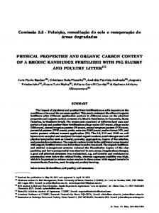
position as the discovery image and were aligned using a simple linear transformation. Assuming the astrometric distortion pattern does not change, the use of the discovery image as part of the parallax solution allows a much shorter dedicated observational campaign to obtain a precise parallax. For CFBDS 0059, SDSS 0207, ULAS 0948 and ULAS 2239 this was not possible because the target was very close to a chip edge in the first UKIDSS image. The WFCAM astrometric distortion is significant, so moving the reference frame on the focal plane results in poorer astrometric transformations (i.e. larger residuals in the solutions) and so in this situation those frames that are significantly offset are given lower weight. Initially all observations were made with the same total exposure time of 400 seconds. For this exposure, in the case of the anonymous stars in the field of ULAS 0034, the centroiding precision is a constant 20mas until around J=18.4 and deteriorates quickly to 60mas at J=19.2 (Figure 2 in SJL10). To ensure that centroiding precision is optimal even in poor observing conditions we have increased the exposure times to 710s for the faint targets (ULAS 0034, 0948, 1150, 1315, 2239 and CFBDS 0059). The precision of the final solutions for the faint targets reflects the poor quality of some of the earlier 400 second observations. In figure 1 we plot the solution of ULAS 0901 (top panel) and 1315 (bottom panel) which are objects of similar distances and observational history but with magnitudes of 17.90 and 18.86 respectively, e.g. straddling the precision borderline, to show high and low quality solutions.

3. Results The astrometric parameters derived for the 11 targets are in Table 2. For each one we report: target name, position (J2000), number of reference stars, number of observations used, absolute parallax, proper motion components, tangential velocity, the time span covered by the observations and the relative-to-absolute parallax correction applied.The proper motion of the targets have all been brought to an absolute system using the galaxies in the field. The relative errors for most of the targets are less than 10%. Observations are continuing and we hope to be able to reduce them to 5% by the end of the campaign. Significant exceptions are ULAS 1150, 1315 and 2239 which are also amongst the faintest objects under study, hence degraded the most by the borderline signal-to-noise in the early observations. In addition, parallax observations of ULAS 2239 were shifted from the discovery image position lowering the weight of the first point. In Table 3 we compare the astrometric distances obtained here with the estimated ones given in the discovery paper of each object. The estimations were made with different techniques and the reader is referred to the discovery papers (see footnote to Table 1) for further details. The discovery distance range is usually much larger than our measured one and is overestimated for the late-Ts. This comparison underlines the need for measured parallaxes that are model independent.

4. Model Fitting In Figs. 2 and 3 we present four color - absolute magnitude diagrams for a sample of L and T dwarfs with M J > 12 and MK > 12 respectively. The 11 targets are plotted as filled circles. Parallaxes and magnitudes of the other objects are from two on-line archives: 1) The L/T dwarf archive maintained by S. K. Leggett

Fig. 1. Observations for the targets ULAS 0901 (top panel) and 1315 (bottom panel). The highest point is the discovery image. The observational history and distance of these two targets are similar but they differ by a magnitude in apparent brightness. The solution shows the effect of low signal-to-noise observations in the beginning of the parallax sequence.

(http://staff.gemini.edu/∼sleggett/2010 phot tab.txt, hereafter Leggett archive): This archive contains a compendium of 225 objects with MKO YJHKL’M’ magnitudes and IRAC [3.55], [4.49], [5.73] and [7.87] magnitudes. Where used these objects are plotted as filled squares. 2) The M/L/T dwarf archive (www.dwarfarchives.org, hereafter Dwarf archive): This is an on line compendium of all published L/T dwarfs and selected M dwarfs. As of 10/01/2010 there were 752 L & T dwarfs, reporting JHK magnitudes, parallaxes and proper motions. Where used these objects are plotted as filled triangles. To make Figs. 2 and 3 clearer we omitted the error bars on the literature objects. An indication of the typical uncertainty on these points is given by the black cross above the legend.

F. Marocco et al.: Properties of 11 T dwarfs

3

Table 1. Infrared magnitudes and spectral types of the 11 targets. Full Name ULAS J003402.77-005206.7 CFBDS J005910.90-011401.3 SDSS J020742.48+000056.2 ULAS J082707.67-020408.2 ULAS J090116.23-030635.0 ULAS J094806.06+064805.0 ULAS J101821.78+072547.1 ULAS J115038.79+094942.8 ULAS J131508.42+082627.4 ULAS J133553.45+113005.2 ULAS J223955.76+003252.6

zAB 22.11 ± 0.05 21.93 ± 0.05 20.11 ± 0.60 ... ... ... ... 22.44 ± 0.10 22.82 ± 0.10 22.04 ± 0.10 ...

Y 18.90 ± 0.10 18.82 ± 0.02 17.94 ± 0.03 18.29 ± 0.05 18.82 ± 0.05 20.03 ± 0.14 18.90 ± 0.08 19.92 ± 0.08 20.00 ± 0.08 18.81 ± 0.04 19.94 ± 0.17

J 18.15 ± 0.03 18.06 ± 0.03 16.75 ± 0.01 17.19 ± 0.02 17.90 ± 0.04 18.85 ± 0.07 17.71 ± 0.04 18.68 ± 0.04 18.86 ± 0.04 17.90 ± 0.01 18.85 ± 0.05

H 18.49 ± 0.04 18.27 ± 0.05 16.79 ± 0.04 17.44 ± 0.05 18.46 ± 0.13 19.46 ± 0.22 17.87 ± 0.07 19.23 ± 0.06 19.50 ± 0.10 18.25 ± 0.01 19.10 ± 0.10

K 18.48 ± 0.05 18.63 ± 0.05 16.71 ± 0.05 17.52 ± 0.11 > 18.21 > 18.62 18.12 ± 0.17 19.06 ± 0.05 19.60 ± 0.12 18.28 ± 0.03 18.88 ± 0.06

Sp. Type T9 T9 T4.5 T5.5 T7.5 T7 T5 T6.5p T7.5 T9 T5.5

Refs (D,P,T) 1,1,6 2,2,6 3,(4,7),8 4,4,4 4,4,4 4,4,4 4,4,4 5,5,5 5,5,5 6,6,6 4,4,4

YJHK are in the MKO Vega photometric system, while z is in AB system. The uncertainty in the spectral type is ±0.5. References (D = Discovery, P = Photometry, T = Spectral Type): 1- Warren et al. (2007) 2- Delorme et al. (2008) 3- Geballe et al. (2002) 4Lodieu et al. (2007) 5- Pinfield et al. (2008) 6- Burningham et al. (2008) 7- Knapp et al. (2004) 8- Burgasser et al. (2006)

Table 2. Parallaxes and proper motions of the 11 targets. Target ULAS 0034 CFBDS 0059 SDSS 0207 ULAS 0827 ULAS 0901 ULAS 0948 ULAS 1018 ULAS 1150 ULAS 1315 ULAS 1335 ULAS 2239

α (h:m:s) 0:34:02.7 0:59:10.9 2:07:42.9 8:27:07.6 9:01:16.2 9:48:06.1 10:18:21.7 11:50:38.7 13:15:08.4 13:35:53.4 22:39:55.7

δ (d:m:s) - 0:52:07.8 - 1:14:01.4 + 0:00:56.0 - 2:04:08.4 - 3:06:35.4 + 6:48:04.5 + 7:25:46.8 + 9:49:42.8 + 8:26:27.0 +11:30:05.1 + 0:32:52.7

N*, obs 135, 17 70, 13 47, 17 418, 17 241, 19 152, 15 198, 14 105, 10 213, 11 196, 8 120, 15

πabs ± σπ (mas) 78.0 ± 3.6 108.2 ± 5.0 29.3 ± 4.0 26.0 ± 3.1 62.6 ± 2.6 27.2 ± 4.2 25.0 ± 2.0 16.8 ± 7.5 42.8 ± 7.7 96.7 ± 3.2 10.4 ± 5.2

µabs α ± σµ α (mas/y) -18.5 ± 3.2 878.8 ± 8.4 158.8 ± 3.0 26.8 ± 2.7 -38.6 ± 2.3 199.4 ± 7.0 -183.7 ± 2.6 -107.6 ± 17.1 -60.2 ± 8.3 -196.9 ± 4.9 125.3 ± 5.4

µabs δ ± σµ δ (mas/y) -363.3 ± 3.6 50.5 ± 4.8 -14.3 ± 3.9 -108.9 ± 2.3 -261.2 ± 2.8 -273.9 ± 6.2 -15.1 ± 3.1 -31.9 ± 4.5 -95.8 ± 10.0 -201.0 ± 6.3 -108.4 ± 5.2

Vtan (km/s) 21.7 ± 1.0 38.6 ± 1.8 25.8 ± 3.6 20.5 ± 2.5 20.0 ± 0.8 59.1 ± 9.3 34.9 ± 2.8 31.7 ± 14.9 12.5 ± 2.5 13.8 ± 0.5 75.7 ± 37.8

Time span (years) 3.81 2.69 3.70 3.94 3.90 1.58 2.00 2.91 3.07 2.18 2.95

COR (mas) 1.24 1.19 1.37 0.87 1.00 0.98 1.04 1.09 0.95 0.95 0.96

In the fourth column we report the number of reference stars (N*) and the number of observations (obs). In the ninth column we report the time span covered by the observations and in the last one the relative-to-absolute parallax correction (COR).

Table 3. The 1-sigma distance range obtained here compared to those estimated in the discovery papers. Name ULAS 0034 CFBDS 0059 ULAS 0827 ULAS 0901 ULAS 0948 ULAS 1018 ULAS 1150 ULAS 1315 ULAS 1335 ULAS 2239

Astrometric distance (pc) 12.2-13.4 8.8-9.6 33.8-43.0 15.3-16.7 31.1-42.5 36.8-43.2 32.9-86.1 19.2-27.6 10.0-10.6 48.0-144.2

Discovery distance (pc) 14-24 8-18 24-39 21-33 38-60 33-52 42-60 34-48 8-12 52-83

Discovery reference 1 2 3 3 3 3 4 4 5 3

References: 1- Warren et al. (2007) 2- Delorme et al. (2008) 3Lodieu et al. (2007) 4- Pinfield et al. (2008) 5- Burningham et al. (2008)

All magnitudes are in the MKO system and preferentially taken from the Leggett archive as they are measured directly in that system. The majority of the infrared magnitudes in the Dwarf archive are in the 2MASS system and when needed we use the relations in Stephens & Leggett (2004) to convert to the MKO system. Colored lines in Figs. 2 and 3 are the model predictions by Burrows et al. (2006, hereafter BSH06) and Allard et al.

(2003, 2007, 2009, hereafter BTSettl09). BSH06 tracks covers the temperature range 700-2000 K, with log[g]=4.5,5.0,5.5 and [Fe/H]=-0.5,0,+0.5. BTSettl09 covers the range 500-780 K, with log[g]=4.5,5.0,5.25 and [Fe/H]=-0.2,0,+0.2. For a given metallicity (indicated in the plots by a given color) log[g] increases from left to right in J-H, while it increases from right to left in J-K. Model colors and magnitudes were obtained by convolving the theoretical spectra with the UKIDSS filter profiles (Hewett et al. 2006) to calculate fluxes. We interpolate the model spectra with a spline to have the same binning as the filter profiles, apply the selected profile, and integrate to obtain the total flux. The integrated fluxes were then converted into an absolute magnitude using as a zero point a Vega spectrum treated the same way. The absolute magnitudes plotted in Figs. 2 and 3 require from the models the flux at 10 pc. The BSH06 models supply the flux at the surface of the object and at 10 pc, the latter calculated assuming the radius-log(g)-Te f f relation from Burrows et al. (1997). The BTSettl09 models provide only the flux at the surface of the object, to find the flux at 10pc we assume the radii from Baraffe et al. (2003) corresponding to the model log(g) and effective temperature. In Figs. 2 and 3 we note that the BTSettl09 tracks for high and low metallicity are swapped in the different color spaces. In J-H space tracks for high metallicity are bluer than the low metallicity ones, while in J-K they are redder. This follows the trend suggested by BSH06 tracks for higher temperature, and

4

F. Marocco et al.: Properties of 11 T dwarfs

can be seen also in the models of Saumon & Marley (2008). Due to this swap, the predictions for the T9 dwarfs are incompatible in the two color spaces, i.e. they predict high gravity - low metallicity in J-H and low gravity - high metallicity in J-K. Moreover, the T9s are redder than predicted by the theoretical models, especially in J-K. This failure may be due to an incorrect prediction of the flux emitted in the H and K-band resulting from known opacity deficiencies in modeling the collision-induced absorption of H2 and the wing of the K I doublet resonance, and the lack of an appropriate list of absorption lines of CH4 and NH3 at such low temperatures (Leggett et al. 2010). The predictions for earlier objects are consistent in the two color spaces, but in Fig. 2 they tend to slightly underestimate the magnitudes of the T6.5-T7s. Further discussion on the models predictions and individual objects is in Section 6. In Fig. 4 we present three absolute magnitude - IR spectral type diagrams. The IR spectral type classification follows the scheme described in Geballe et al. (2002) for L dwarfs and the scheme described in Burgasser et al. (2006) for T dwarfs. The over plotted curves are polynomial fits derived in Liu et al. (2006), with the dotted line representing the polynomial obtained excluding from the fit all the known and possible binaries, while the dashed line is the one obtained excluding only the known binaries. Possible binaries were selected by Liu et al. based on their relatively high Te f f compared to objects of similar spectral type in the Golimowski et al. (2004) measurements. One of the possible binaries indicated by Liu et al. (SDSS J10210304) was confirmed as a binary by Burgasser et al. (2006), so now is plotted as a known binary. Following the convention used before, filled circles are the 11 targets and squares are objects from the Leggett archive, while blue objects are known binaries and green objects are possible binaries. The trend for T8.5 and T9 is an extrapolation of the Liu et al polynomial, since their sample consisted of objects between L0 and T8. The 11 targets indicate a steeper trend in the sequence beyond T8 than the extrapolation of the Liu et al. polynomial. In Fig. 4 the red lines are our 4-th order polynomials fit to the data including the new objects presented here, but excluding the 14 objects without magnitude naturally in the MKO system. This choice was made as the Stephens & Leggett (2004) transformations from the 2MASS to the MKO system were derived using hotter objects and employing them may introduce systematic errors in the resulting fit of the cooler objects. In Table 4 we list the coefficients and errors of the fit. The difference between the two fits with and without possible binaries is reduced compared to Liu et al., probably because of the smaller statistical weight of the possible binaries in this study (5 over a total sample of 61 objects) with respect to Liu et al. (6 over 43). As the sample of late T dwarfs is still small, identification of possible binaries in this region may be incomplete. We also tested polynomials from 3rd to 10th order but after 4th order there was no significant improvement in the sigma of the fit.

5. Luminosity and Effective Temperature. Next we calculate an effective temperature range for our targets. To do this we used the classical Stefan-Boltzmann law: Lbol = 4πσR2 T e4f f

(1)

hence to calculate the temperature we need to know the radius and the bolometric luminosity of each object. To determine a radius, we consider the models of Baraffe et al. (2003) we see that the radius of T dwarfs decreases

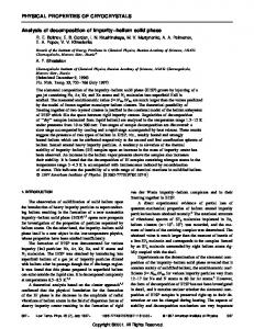
rapidly when the object is very young but after 0.5 Gyr it is very constant. Therefore if we can constrain the age of our objects we can use these models to constrain the radius. In Fig. 5 we report the galactic velocity components (U,V,W) of the 11 targets. The components were calculated from the proper motions in Table 2 assuming a radial velocity range of +80/-80 km/s. Given this large range in Vrad , the uncertainty in the proper motion becomes negligible, so we ignore it in this calculation. The overplotted box is the locus of very young objects (age < 0.1 Gyr, Zuckerman & Song 2004) while the ellipsoid is the locus of young disk objects (age < 0.5 Gyr, Eggen 1969). Even given this very conservative range in possible radial velocities no objects fall in the boxed area or in the ellipsoid area in all three components. We therefore conclude that all objects are older than 0.5 Gyr. For the 0.5-10 Gyr models from Baraffe et al. (2003) we find the radius has a range of 1.2 - 0.8 R Jup (in a temperature range of 500 - 2000 K). This is also consistent with the radii predicted by Burrows et al. (1997) models for objects of the same age and temperature. To calculate the bolometric flux (and hence the luminosity) we combined the available measured spectrum of each object (Burningham et al. 2008; Leggett et al. 2009) flux calibrated using UKIDSS YJHK photometry, with the model spectra. For ULAS 0034 and 1335 we have the spectrum in the near- and mid-infrared (hereafter MIR) region, while for the other objects we only have the NIR portion. To find the bolometric flux we use model spectra to estimate the flux where we do not have observations: at short wavelengths (λ < 1.0 µm), and, for ULAS 0034 and 1335, in the region between the near- and mid-infrared spectrum (2.4 µm < λ < 7.5 µm) or, for the other targets, in the entire portion from 2.4 µm to 15 µm. The flux emitted beyond 15 µm was estimated assuming a Rayleigh-Jeans tail. The models used are the already mentioned BTSettl09 and the non-equilibrium models by Hubeny & Burrows (2007), covering the temperature range from 700 to 1900 K, for log[g]=4.5,5.0 and 5.5, assuming values of Kzz =102 ,104 and 106 cm2 s−1 (eddy diffusion coefficient), for different speed of the CO/CH4 reaction (for further details see Hubeny & Burrows 2007; Saumon et al. 2006 and reference therein). For each object we took the models in a wide range of temperature (±200 K around the temperature predicted by the temperature-type relation given by Stephens et al. 20091 ), gravity (log[g] from 4.5 to 5.5) and metallicity ([Fe/H] from -0.2 to +0.2) and we scaled them using the available magnitudes (listed in Tables 1 and 5). For each model we took the average scaling factor obtained and we compared it with the range given by the known distance and the radius range adopted (i.e. the square of 0.8 R Jup /distance ± 3σ - the square of 1.2 R Jup /distance ± 3σ). We discarded the models whose average scaling factor was out of this pseudo-3σ range. We joined each one of the remaining spectra with the measured one and we calculate the resulting bolometric flux, the luminosity and hence the temperature range (corresponding to the radius range). Then we compared the temperature obtained with the one associated with the model employed. We discarded those models whose temperature differed by more than 100 K from the temperature range obtained. Finally we assumed the mean flux given by the remaining models as our final estimation and hence we calculate the luminosity and the temperature range. The uncertainty in the flux is given by the spread in values plus a 3% uncertainty in the magnitudes used to calibrate the 1 Except for the T9s, since we don’t have theoretical spectra for temperatures lower than 500 K.

F. Marocco et al.: Properties of 11 T dwarfs

5

Fig. 2. Color-magnitude diagrams for a sample of L and T dwarfs. The colored lines are theoretical tracks from BSH06 and BTSettl09, for different gravities and metallicities. For each metallicity, the gravity increases from left to right, assuming the values 4.5,5.0,5.5 for BSH06 tracks and 4.5,5.0,5.25 for BTSettl09. The 11 targets presented here are plotted as filled circles with their associated error bars, the Dwarf archive objects are plotted as triangles and the Leggett archive objects as squares. All magnitudes in the MKO system. The cross above the legend indicates the typical uncertainty on the literature objects. observed spectra and to scale the model ones. The uncertainty in the luminosity and the temperature is the result of the standard propagation of the errors on the flux and the distance, ignoring the uncertainty in the radius, given the wide range adopted.

The results are shown in Table 6. In the first column we indicate the target short name, in the second one its spectral type, in the third the temperature estimated using the temperaturespectral type relation given by Stephens et al. (2009), in the fourth the range of models employed, in the fifth the range of

6

F. Marocco et al.: Properties of 11 T dwarfs

Fig. 3. Same as Fig. 2 but with the color J-K instead of J-H. For each metallicity, the gravity increases from right to left, assuming the values 4.5,5.0,5.5 for BSH06 tracks and 4.5,5.0,5.25 for BTSettl09. models kept after the first step (so after comparing the scaling factors), in the sixth the range of models kept after the second step (so after comparing the temperatures), in the seventh our assumed bolometric flux, in the eighth the associated luminosity and in the last the temperature range obtained. We note that the use of MIR magnitudes and spectra increases our ability to constrain the object temperature. For ULAS 0034 and 1335 the bolometric flux is well constrained

and the width of the temperature range obtained (150-200 K) is mainly due to the radius. Using the NIR spectrum and photometry only, the uncertainty on the flux increases and the temperature range obtained doubles.

To have an idea of the eventual systematics, we also tested the technique described in Cushing et al. (2008), e.g. to fit the

F. Marocco et al.: Properties of 11 T dwarfs

7

Fig. 4. J, H and K-band absolute magnitude as a function of IR spectral type. Labeled objects are those with new parallaxes presented here. Blue squared points are known to be unresolved binaries, while green squared points are possible unresolved binaries. The over plotted lines are polynomial fit by Liu et al. (2006) based on data tabulated by Knapp et al. (2004). The dotted line was obtained excluding all the known and possible binaries, the dashed one excluding only the known binaries. The red lines are our new polynomial fits.

8

F. Marocco et al.: Properties of 11 T dwarfs

Table 4. Coefficients of the polynomial fit. Magnitude

a0

MJ MH MK

11.140 ± 0.052 10.486 ± 0.051 10.180 ± 0.056

MJ MH MK

10.957 ± 0.053 10.292 ± 0.052 10.005 ± 0.056

a1 a2 a3 Excluding known and possible binaries 0.556 ± 0.032 3.74 ± 0.62 ×10−2 -9.49 ± 0.45 ×10−3 0.590 ± 0.031 -3.80 ± 0.61 ×10−3 -4.35 ± 0.44 ×10−3 0.375 ± 0.035 2.31 ± 0.67 ×10−2 -5.03 ± 0.49 ×10−3 Excluding known binaries 0.736 ± 0.032 -5.53 ± 0.61 ×10−3 -6.31 ± 0.44 ×10−3 0.778 ± 0.031 -4.77 ± 0.60 ×10−2 -1.13 ± 0.43 ×10−3 0.548 ± 0.034 -1.84 ± 0.64 ×10−2 -1.93 ± 0.46 ×10−3

a4 3.69 ± 0.11 ×10−4 2.15 ± 0.11 ×10−4 2.11 ± 0.12 ×10−4 2.96 ± 0.11 ×10−4 1.41 ± 0.10 ×10−4 1.38 ± 0.11 ×10−4

P The fits are defined as in Liu et al. (2006): MXX = 4i=0 ai × (SpT)i where XX indicates J, H or K-band magnitude and the spectral types are defined following the convention SpT=1 for L1, SpT=9 for L9, SpT=10 for T0 etc. The fit is valid for spectral types from L0 to T9. Infrared spectral types are used for both L and T dwarfs.

Table 6. Fluxes, luminosities and temperatures of the sample obtained scaling the model spectra using the measured magnitudes, e.g. the first method discussed in Section 5. object ULAS 0034 CFBDS 0059 SDSS 0207 ULAS 0827 ULAS 0901 ULAS 0948 ULAS 1018 ULAS 1150 ULAS 1315 ULAS 1335 ULAS 2239

Sp. Type T9 T9 T4.5 T5.5 T7.5 T7 T5 T6.5p T7.5 T9 T5.5

est. Te f f (K) 500 500 1130 1070 830 910 1100 980 830 500 1070

models used (K) 500:700 500:700 900:1400 900:1300 600:1000 700:1100 900:1300 800:1200 600:1000 500:700 900:1300

1st step (K) 540:700 500:620 1000:1400 1000:1300 600:700 700:800 900:1100 800:1200 600:740 540:660 900:1300

2nd step (K) 540:660 500:620 1100:1200 1000:1100 600:700 700:800 900:1000 900:1000 600:660 540:660 1100:1200

Table 5. IRAC magnitudes of ULAS 0034, SDSS 0207 and ULAS 1335 (Warren et al. 2007; Patten et al. 2006; Burningham et al. 2008) used to scale the model spectra. 3.55 µm 4.49 µm 5.73 µm 7.87 µm

ULAS 0034 16.28 ± 0.49 14.49 ± 0.43 14.82 ± 0.44 13.91 ± 0.42

SDSS 0207 15.59 ± 0.06 14.98 ± 0.05 14.67 ± 0.20 14.17 ± 0.19

ULAS 1335 15.96 ± 0.48 13.91 ± 0.42 14.34 ± 0.43 13.37 ± 0.41

object spectrum using the model spectra. The best fit spectrum was selected as the one that minimize: ! n X fi − Ck Fk,i 2 (2) Gk = wi σi i=1 where n is the number of data pixels, fi is the measured flux in the i-th spectral interval, Ck is the scaling factor (R/d)2 , Fk,i is the k-th model flux and σi is the error in the measured spectrum. The weight associated to each bin (wi ) is the extension of the bin itself (∆λ) as suggested by Cushing et al. The scaling factor can be provided by the fit, however, since we know the distance to the dwarf we consider fixed values of Ck , assuming again the radius range previously indicated. We selected the best fit models for the two extreme configurations, i.e. 0.5 Gyr-1.2 R Jup and 10 Gyr-0.8 R Jup . Since we don’t have an associated noise spectrum for ULAS 0827, 0948, 1018, 1150, 1315 and CFBDS 0059 we minimize:   n X  fi − Ck Fk,i 2 Gk = wi  (3)  p fi i=1

Fbol (erg s−1 cm−2 ) 2.34±0.05×10−13 2.85±0.48×10−13 4.98±0.26×10−13 2.87±0.09×10−13 1.88±0.15×10−14 6.52±0.44×10−14 1.80±0.43×10−13 6.76±0.40×10−14 7.47±0.72×10−14 3.42±0.09×10−13 6.00±0.09×10−14

L/L⊙ 1.13±0.06×10−6 7.20±1.25×10−7 1.72±0.25×10−5 1.21±0.15×10−5 1.42±0.13×10−6 2.61±0.44×10−6 8.54±0.70×10−6 7.12±3.22×10−6 1.21±0.25×10−6 1.09±0.06×10−6 1.65±0.82×10−5

Te f f range (σ) (K) 535 - 660 (35) 480 - 590 (55) 1060 - 1300 (110) 970 - 1190 (95) 570 - 700 (50) 660 - 810 (80) 890 - 1090 (75) 850 - 1040 (160) 545 - 670 (70) 530 - 650 (35) 1050 - 1280 (200)

The uncertainty in the extremes takes into account half of the models grid spacing based on fitting (for further details see Cushing et al.), plus an additional percentage on the flux due to the incomplete spectral coverage. This percentage was estimated comparing the measured IRAC magnitudes of ULAS 0034 and 1335 with the model’s predicted ones. The differences between measured and model magnitudes gives an average uncertainty of ∼70% on the calculated flux between 2.5 and 7.5 µm. For ULAS 0034 and 1335 in this interval there is ∼40% of the total emergent flux, so we obtain a relative error σF,rel =.7×.4=.28. This implies an additional uncertainty of ∼7% on the temperature. For the other 9 objects, the uncertainty in the temperature was estimated extending the relative sigma calculated for ULAS 0034 and 1335 to the uncovered part of the flux (∼60%, that results in an uncertainty σF,rel =.7×.6=.42). The choice of the weight function is arbitrary. Different choices can lead to different results, as seen by Cushing et al. (2008) and Stephens et al. (2009). Given this, we prefer the results obtained with the first method described. The values obtained with this spectral technique are summarized in Table 7. They are largely consistent with the ones obtained scaling the model spectra. We also performed a completely model independent flux calculation for ULAS 0034 and 1335, that have a completely measured spectral energy distribution. We determined the bolometric flux emitted integrating the measured spectrum between 1 and 2.5 µm, then adding the flux emitted between 2.5 and 7.5 µm calculated using the IRAC magnitudes (assuming a constant flux distribution over the passband2), finally we integrated the mea2 Any error that this assumption may introduce would be negligible, since the IRAC passbands are tight.

F. Marocco et al.: Properties of 11 T dwarfs

9

Table 7. Temperatures obtained fitting the observed spectrum, e.g. the second method discussed in Section 5. Name

Sp. Type

ULAS 0034 CFBDS 0059 SDSS 0207 ULAS 0827 ULAS 0901 ULAS 0948 ULAS 1018 ULAS 1150 ULAS 1315 ULAS 1335 ULAS 2239

T9 T9 T4.5 T5.5 T7.5 T7 T5 T6.5p T7.5 T9 T5.5

Te f f range (σ) (K) 500 - 580 (40) 500 - 540 (60) 1000 - 1200 (120) 1100 - 1200 (130) 620 - 720 (75) 700 - 800 (90) 900 - 1100 (120) 800 - 1000 (110) 540 - 620 (65) 500 - 600 (40) 1100 - 1300 (135)

Fig. 6. Temperature ranges plotted as a function of the spectral type. Uncertainties in each extreme point of the range are in Table 6. The uncertainty in spectral type is half subtype. The over plotted dotted line is the effective temperature-infrared type relation derived by Stephens et al. (2009). sured 7.5 - 15 µm spectrum. The flux emitted beyond 15 µm was estimated assuming a Rayleigh-Jeans tail. The results obtained for ULAS 0034 and 1335 with this approach are consistent with the one obtained with the other techniques described within the uncertainty quoted in Table 6.

6. Discussion

Fig. 5. The galactic velocity components U, V and W obtained from the proper motions in Table 2 assuming a Vrad range of +80/-80 km/s. The triangle indicates the +80 km/s extreme, the diamond indicates the -80 km/s extreme. The overplotted black box is the locus of young stars (Zuckerman & Song 2004, age< 0.1 Gyr), the ellipsoid is the locus of young disk stars (Eggen 1969, age< 0.5 Gyr).

In Fig. 6 we present a Te f f -spectral type diagram of the 11 Tdwarfs of the sample, for each of which we plot the temperature range displayed in Table 6. When needed, objects have been offset by ±0.1 in spectral type, to avoid overlaps. Over plotted for comparison we have the effective temperature - infrared type relation derived by Stephens et al. (2009). All the ranges are consistent with the relation except for ULAS 0948, 0901 and 1315, that are cooler than predicted. We now discuss individual objects with temperature values or indications of peculiarity in the literature. 6.1. ULAS 0034

There are several estimations of the temperature of this object. In the discovery paper, Warren et al. (2007) estimate a conservative range of 600 ≤ Te f f ≤ 700 K using the measured NIR

10

F. Marocco et al.: Properties of 11 T dwarfs

spectrum and the near- and mid-infrared photometry with a grid of solar-abundance BTSettl model, calibrated using the parameters of 2MASS0415, and a linear fit of Te f f vs. H-[4.5] color for hotter stars; Delorme et al. (2008) using the NIR spectrum and the same grid described in Warren et al. (2007) determine Te f f ≈ 670 K; in Leggett et al. (2009) the published range is 550 ≤ Te f f ≤ 600, obtained fitting the measured NIR and MIR spectrum with model spectra by Saumon & Marley (2008); finally, in SJL10 using the parallax reported in this paper and the model fitting in Leggett et al. (2009), using a model radius of 0.11 R⊙ (as implied by the spectral fits constraints on gravity), derive a bolometric luminosity of L/L⊙ =1.10±0.01×10−6, consistent with the temperature range 550-600 K. In this work, using NIR and MIR spectrum, the MKO NIR photometry and the IRAC MIR photometry, we find a luminosity of L/L⊙ =1.13±0.06×10−6, consistent with the value obtained by Leggett et al. (2009). The difference between the temperature range derived here and by Leggett et al. is due to the different technique used: the Leggett et al. spectral fitting result is similar to that derived spectrally here, given in Table 7. 6.2. CFBDS 0059

In the discovery paper (Delorme et al. 2008) of this object they estimate Te f f ∼620 K comparing the spectral indices with a solar metallicity grid of BTSettl model spectra. In Leggett et al. (2009) the technique adopted is the same described in Sec. 6.1, and the range obtained is 550