Parallel Algorithm for On-Line Ranking in Trees

Parallel Algorithm for On-Line Ranking in Trees Chia-wei Lee and Justie Su-tzu Juan Department of Computer Science and Information Engineering National Chi Nan University, Puli, Nantou 545, Taiwan, R.O.C. {s2321513, jsjuan}@ncnu.edu.tw Abstract A node k-ranking of a graph G = (V, E) is a proper node coloring C: V  {1, 2, …, k} such that any x-y path in G with C(x) = C(y) contains an internal node z with C(z) C(x). In the on-line version of this problem, the nodes v1, v2, …, vn are coming one by one in an arbitrary order; and only the edges of the induced subgraph G[{v1, v2, …, vi}] are known when the color of vi has to be chosen. This paper gives an on-line ranking algorithm for general trees in parallel with O(nlog2n) time using O(n3/log2n) processors on CREW PRAM model, and the cost is O(n4).

1

Introduction

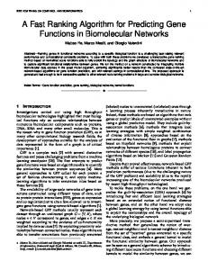
In this paper we discuss node ranking of graphs. The investigation of node ranking problem, also called ordered coloring problem [10], has important in computing Cholesky factorizations of matrices in parallel (see [2], [5], [14]), scheduling problem of assembly steps in manufacturing systems (see [7], [8], [18]), and finding the minimum-height elimination tree of a graph (see [4], [18]). Yet other applications lie in the field of VLSI-layout (see [12], [17]). Now we define the node ranking problem theoretically. Let G = (V, E) be a simple graph with node set V and edge set E. A node k-ranking (or ranking for short) of G is a proper node coloring C: V  {1, …, k} such that every path in G with end nodes x and y of the same color C(x) = C(y) contains a node z with greater color C(z)  C(x). The ranking number r(G) is the smallest integer k for which there exists a node k-ranking of G. A node k-ranking C of G is called optimal if max{C(x)|x V(G)} = r(G). Figure 1 shows an example — a node 4-ranking of a tree.

4

v2

1 v1 3 v3

2 v6

1

v4

4

v7

5

v5

1

v8

1

Figure 2: An example for on-line version In the off-line version of node ranking problem, Katchalski, McCuaig, and Seager [10] showed that r(Pn) =  log2n+ 1, for n 1, where Pn is a path with n nodes. And Bruoth and Horň á k [3] proved r(Cn) =  log2(n –1)+ 2, for n [3, ], where Cn is a cycle with n nodes. Iyer, Ratliff, and Vijayan [6] showed that the ranking number of trees has a good upper bound log3/2(n), and they also gave an node log3/2(n)-ranking with time complexity in O(nlogn) for trees, where n is the number of nodes.

1

2 1

The graph G is called on-line k-rankable if there is an algorithm that generates a k-ranking of G for every possible input sequence of the nodes of G. That means nodes of a graph G are coming in an arbitrary order. The nodes of the graph G are colored one by one in such a way that only a local information concerning edges between already present nodes is known in the moment when a color for a node is to be chosen. The assigned color cannot be changed later. The on-line ranking number r*(G) is the smallest positive integer k such that G is on-line k-rankable. The situation for on-line ranking is different to the off-line version, since some input sequences require more colors than off-line version. Figure 2 shows an example for on-line version with more colors than off-line version when we use Greedy (First-fit) algorithm. Actually, Bruoth and Horň á k showed that r*(P5) = 4 > 3 = r(P5) in [3].

1 3

2 1

Figure 1: A node 4-ranking of a tree.

Theorem 1.1 [6]: Let T be a tree with n nodes. Then r(T)  log3/2(n).

Schäffer improved their work on [16], obtained a linear time algorithm for finding a node log3/2(n)-ranking of a tree. Except paths, cycles, and trees, Yu discussed this problem for cographs in 1994 [20]. Wang and Yu discussed this problem for interval graphs in 1996 [19]. Liang, Dhall and Lakshmivarahan discussed this problem in parallel [15]. They proposed a fast parallel algorithm for finding approximate optimal node ranking of trees using O(logn) steps with n2 processors on CREW PRAM and an efficient parallel algorithm using O(log2n) steps with n processors on EREW PRAM model. And in [13], Liu and Yu presented a parallel algorithm which needs O(logn) time and n/logn processors on the EREW PRAM model for this problem on cographs. In the on-line version, there are few results until now. In [3], Bruoth and Horň á k gave the bounds for r*(Pn) and r*(Cn). Theorem 1.2 [3]: 1. For any n  [1, ],  log2n+ 1 r*(Pn)  2 log2n+ 1. 2. For any n [3, ],  log2(n –1)+ 2 r*(Cn) 2 log2n+ 1. In [11], Lee and Juan gave an on-line ranking algorithm for trees. In this paper, we will focus on on-line version in parallel. That is, we will give an on-line ranking algorithm for trees in parallel. This paper is organized as follows: In Section 2, we recall the algorithm for on-line ranking of trees which established in [11]. In Section 3, we give the parallel algorithm for on-line ranking of trees and show the correctness of the algorithm. In Section 4, we analyze this parallel algorithm. Finally, we summarize the results and give some future works in Section 5.

2

Sequential algorithm for trees

In [11], Lee and Juan gave following sequential algorithm A for on-line ranking for trees. We used the idea of Greedy algorithm to develop algorithm A. For each new node was added, we need to choose a suitable color to rank this new node. We used an array for each node help us to record which color cannot be chose to rank its neighbors. After we rank a new node, some color may not be a suitable color for next new node any more. That is, we need to modify these arrays after we rank each new node. We used DFS (Depth-First-Search) technique to modify these arrays.

In algorithm A, an array color_array[vi][j] is used to record a new neighbor of vi can be colored with color j or not, 1 for yes, 0 for not. When each new node was added, Procedure Rank will choose a best suitable color for each new in-coming node and it will call the other two Procedures. The Procedure Color_Array is used to create color array for the new node. The Procedure Modify_Color_Array is used to modify the color array of the old nodes to keep the correctness of color array. Algorithm A [11] {Input: an integer n = the number of nodes of tree T; Output: assignment C of the colors to the nodes}. Begin (1) for k = 1 to n do (1.1) Read new node vk and the neighbors of vk in T[{v1, v2, …, vk–1}] = T*, say u1, u2, …, um; (1.2) for i = 1 to n do color_array[vk][i] = 1; (1.3) Rank(vk); End; //End of Algorithm A Procedure Rank(vk) Begin (1) if m = 0 then (1.1) C(vk) = 1; (1.2) color_array[vk][1] = 0; (2) else (2.1) for j = 1 to n do combine[j] = 1im color_array[ui][j]; (2.2) find the smallest color in which combine[color] = m, and for each i > color, combine[i] m –1; (2.3) C(vk) = color; (2.4) Color_Array(vk, color); (2.5) for i = color to n do if color_array[vk][i] = 0 then Modify_Color_Array(vk, i); End; //End of Procedure Rank Procedure Color_Array(vk, color) Begin (1) for i = 1 to color –1 do color_array[vk][i] = 1; (2) color_array[vk][color] = 0; (3) for i = color + 1 to n do (3.1) if the combine[i] = m then color_array[vk][i] = 1; (3.2) else color_array[vk][i] = 0; End; //End of Procedure Color_Array Procedure Modify_Color_Array(v, i) Begin (1) for any node u adjacent to v do

(1.1) if color(u) i then (1.1.1) color_array[u][i] = 0; (1.1.2) Modify_Color_Array(u, i); End; //End of Procedure Modify_Color_Array From [11], we knew the time complexity of Algorithm A is O(n3). Theorem 2.1 [11]: The output function C of algorithm A is an on-line node ranking of the input tree T.

3

Parallel algorithm for trees

The algorithm B described below will be showed to be an on-line ranking for trees in parallel. This algorithm is designed base on algorithm A. In this parallel algorithm, we consider running in CREW PRAM model. We use five new arrays in this algorithm: mark[i], modify[vk][i], ancestor[vi][vj], n_ancestor[vi], and ANC[vi][j]. The array mark[i] is used to help us when we want to choose a suitable color to color a new node. The modify[vk][i] is used to record color_array[vk][i] is need to be renew or not when a new node be colored, 1 for yes, 0 for not. The ancestor[vi][vj] is recorded whether node vj is an ancestor of node vi or not, 1 for yes, 0 for not. The n_ancestor[vi] is used for record the number of ancestors of node vi. And the ANC[vi][j] saved the sum of modify[vm][j], where vm is an ancestor of vi for color j. Besides, we also use some well known parallel techniques, like Prefix Computation and Interval Broadcasting. The input of Prefix Computation is an array of n element x1, x2, …, xn, and the output is the prefix sum si, for 1 i n. It can be done in O(logn) using O(n/logn) processors. The input of Interval Broadcasting is an array X of n elements. Certain positions of X are referred to as leaders which hold a datum. The positions of the leaders are entirely arbitrary. It is required to copy the datum in each leader into all positions of the array following the leader, up to, but not including, the next leader (if it exists). The Interval Broadcasting can be performed in O(logn) using O(n/logn) processors. We also use Euler tour technique and its application in Procedure Ancestor. This procedure is used to find ancestors for each node in tree. It is help us to modify color_array. After running this procedure when given a tree T* rooted at vk, we have a k k matrix which records whether vi is an ancestor of vj. We use ancestor[vi][vj] to represent whether vi is an ancestor of vj, 1 for yes, 0 for not.

Given the preorder of the tree and the descendants of node vj, the question whether vi is an ancestor of vj can be answered in constant time using one processor. Since we use the results of Euler tour to perform the preorder of the tree T*, the parents of every node, and the descendants of every node in O(logn), O(1), O(1) with using O(n) processors. And to find the Euler tour can be done in O(1) using O(n) processors. Hence, the Procedure Ancestor can be done in O(logn) using O(n/logn) processors. All of these parallel techniques can be found in [1] or [9]. In the step (2.2) of Procedure Rank in algorithm A, we want to find the suitable color. And it needs O(n) time in sequential method. But in parallel method, we use some parallel techniques help us to choose the suitable color. And the time complexity for this procedure will be reduced to O(logn). The next important procedure, Procedure Modify_Color_Array, will be transform to parallel form in similar way. It needs O(n2) time in sequential method. Because the DFS method is the bottleneck of this procedure, we modify this procedure according to its information of ancestors for each node. Then, the time complexity for this procedure will be reduced to O(log2n). Algorithm B /* Parallel Algorithm for on-Line Ranking of Tree */ {Input: an integer n = the number of nodes of tree T; Output: assignment C of the colors to the nodes}. Begin (1) for k = 1 to n do (1.1) Read new node vk and the neighbors of vk in T[{v1, v2, …, vk–1}] = T*, say u1, u2, …, um; (1.2) for i = 1 to n pardo color_array[vk][i] = 1; (1.3) Rank(vk); End; //End of Algorithm B Procedure Rank(vk) Begin (1) if m = 0 then (1.1) C(vk) = 1; (1.2) color_array[vk][1] = 0; (2) else (2.1) for j = 1 to n pardo Apply Prefix Computation to compute combine[j] = 1im color_array[ui][j]; /* choose a suitable color */ (2.2) for j = 1 to n pardo (2.2.1) if combine[j] < m –1 then mark[j] = 0; (2.2.2) else mark[j] = –1;

(2.3) Apply Interval Broadcasting on mark array for mark[j] = 0; (2.4) for j = 1 to n pardo (2.4.1) if combine[j] = m –1 then (2.4.1.1) mark[j] = 0; (2.4.2) if combine[j] = m and mark[j] = –1 then (2.4.2.1) mark[j] = 1; (2.5) Apply Prefix Computation on mark array; (2.6) for j = 1 to n pardo (2.6.1) if mark[j] = 0 then mark[j] = 1; (2.6.2) else mark[j] = 0; (2.7) Apply Prefix Computation on mark array; (2.8) color = mark[n] + 1; //Find the suitable color (2.9) C(vk) = color; (2.10) Color_Array(vk, color); (2.11) Modify_Color_Array(vk, color); End; //End of Procedure Rank Procedure Color_Array(vk, color) Begin (1) for i = 1 to n pardo (1.1) if i < color then color_array[vk][i] = 1; (1.2) if i = color then color_array[vk][i] = 0; (1.3) if i > color then (1.3.1) if the combine[i] = m then color_array[vk][i] = 1; (1.3.2) else color_array[vk][i] = 0; End; //End of Procedure Color_Array Procedure Modify_Color_Array(vk, color) Begin (1) for i = color to n pardo (1.1) if color_array[vk][i] = 0 then modify[vk][i] = 1; (1.2) for j = 1 to k –1 pardo (1.2.1) if C(vj) < i then modify[vj][i] = modify[vk][i] (1.2.2) else modify[vj][i] = 0; (2) Ancestor(T*, vk); /* Find the ancestors for all nodes in which T* */ (3) for i = 1 to k pardo Apply Prefix Computation to get n_ancestor[vi] = 1kn ancestor[vk][vi]; (4) for i = 1 to k pardo for p = 0 to logn –1 pardo for j = p (n/logn) + 1 to (p + 1)  n/logn pardo (4.1) Apply Prefix Computation to get ANC[vi][j] = 1mk modify[vm][j] where ancestor[vm][vi] = 1; (4.2) if ANC[vi][j]  n_ancestor[vi] then modify[vi][j] = 0; (4.3) if modify[vi][j] = 1 then

color_array[vi][j] = 0; End; //End of Procedure Modify_Color_Array Lemma 3.1: Steps (2.2) to (2.8) which lie in Procedure Rank of Algorithm B are equivalent to step (2.2) which lie in Procedure Rank of Algorithm A. Proof. The step (2.2) which lie in Procedure Rank of Algorithm A is to find the smallest color in which combine[color] = m, and for each i > color, combine[i] m –1. In Procedure Rank of Algorithm B, the step (2.2) is used for avoid to choose a color k suck that combine[k] < m –1. The step (2.3) which apply Interval Broadcasting will let the array mark array to be mark[1] = mark[2] = … = mark[a] = 0, and mark[a + 1] = mark[a + 2] + … + mark[n] = –1 for some 1 a n. That means, for all k a, combine[k] m –1. The step (2.4) is ensured to algorithm must choose the color which combine[color] = m. Then, we apply prefix computation in step (2.5), and we can know if mark[j] = 0, then color j cannot be used certainly. In step (2.6), we exchange 1 and 0 in the values of mark array for succeeding computation. It will help us to compute how many colors cannot be used. In step (2.7), we apply prefix computation again. After this step, we can obtain how many colors cannot be used for rank vk. Finally, in step (2.8), we choose the smallest colorable color to rank vk. Then, we can obtain that the steps (2.2) to (2.8) which lie in Procedure Rank of Algorithm B are equivalent to step (2.2) which lie in Procedure Rank of Algorithm A.  Lemma 3.2: Procedure Modify_Color_Array of Algorithm B is equivalent to Procedure Modify_Color_Array of Algorithm A. Proof. The Procedure Modify_Color_Array of Algorithm A is used to modify color_array of the old nodes to keep the correctness. We used DFS (Depth-First-Search) technique in this procedure. When we begin to modify color_array for old nodes, if we find a node vi with C(vi) > C(vk), then we will continue to modify color_arrays for the children of vi no more. That is, if a node vj has an ancestor with greater color, then color_array of node vj need not to modify. In Procedure Modify_Color_Array of Algorithm B, the step (1) is used to initial the modify array. In step (2), we use Euler tour

technique and its applications to find which nodes are the ancestors for all the nodes in the tree. After this step, we have a k k matrix ancestor[vi][vj], which is recorded whether vi is an ancestor of vj. Then in step (3), we apply prefix computation to compute how many ancestors are there for all nodes in tree T* rooted by vk. In step (4.1), for any 1 j n, we apply Prefix Computation to combine modify[vm][j] for any ancestor vm of vi. And we save this results in ANC[vi][j]. The step (4.2) is used to check each node has any ancestor with greater color than j or not. If there exist one ancestor of vi with greater color than j, then we set its modify array to be 0. Thus, if there are no ancestor of node vi with greater color than vi, then the number of the ancestor vm of vi with modify[vm][j] = 1, we set this number to be ANC[vi][j] is equal to the number of the ancestors of vi. So if ANC[vi][j] is less than the number of the ancestors of vi, then we need not to modify the color_array[vi][j] anymore. Finally, for any old node vi of T* which can not have any new neighbor with color j due to the adding of vk, the value of modify[vi][j] will be 1. Hence, in step (4.3), we set color_array[vi][j] = 0 for this kind node vi and color j. Then, we have already modified the color array of the old nodes to keep the correctness of color array.  Theorem 3.3: Algorithm B is equivalent to Algorithm A. Proof. By Lemma 3.1, we know the steps (2.2) to (2.8) will find the suitable color for new node vk, which is equivalent to the step (2.2) which lies in Procedure Rank of Algorithm A. By Lemma 3.2, we have the Procedures Modify_Color_Array in Algorithms A and B are equivalent. Besides, the other steps of these two algorithms are clearly to see that they are equivalent. Then, we obtain that the Algorithm B is equivalent to Algorithm A.  By Theorem 3.3, we know Algorithm A and B are equivalent. That is, each step in algorithm A can be performed in algorithm B by one or more steps. Hence, we have the following theorem. Theorem 3.4: The output function C of algorithm B is an on-line node ranking of the input tree T.

4

Analysis of Algorithm B

In Procedure Modify_Color_Array, processors may read from the same memory location for

modify[vm][j] at the same time and exclusive write in step (4.1). And it is easy to see that the other steps of Algorithm B are exclusive read and exclusive write. Thus, our parallel algorithm is running in CREW PRAM model. In [1] or [9], we know the time complexity of Prefix Computation and Interval Broadcasting both are O(logk) with using O(k/logk) processors, where k is the size of input array. Then, the time complexity of Algorithm B is evaluated as follows. To combine the m color_array which the m nodes adjacent to vk is O(logm) using O(nm/logm) processors. To find the smallest color from color_array of vk and give a color for vk can be done in O(logn) using O(n) processors. The Procedure Color_Array can be performed in O(1) time using O(n) processors. And we need O(logk) time to find ancestors for each node using O(k2/logk) processors in Procedure Ancestor. Note that the step (4.1) in Procedure Modify_Color_Array will take O(logk logn) time and using O(k (n/logn) (k/logk)) processors. Thus, to performed the Procedure Modify_Color_Array need O(logk logn) time using O((k2 n)/(logk logn)) processors. The time complexity of Algorithm B is simply the sum of the Procedures Color_Array and Modify_Color_Array over all n nodes in the tree. Thus, the time complexity of the algorithm B is 1kn {O(logm) + O(logn) + O(1) + O(logklogn)} = O(nlog2n). And the number of processors that we need is max1kn max{O(nm/logm), O(n), O(n), O(k2/logk), O(k2n/logklogn)} = O(n3/log2n). Then, this parallel algorithm can be performed in O(nlog2n) time using n3/log2n processors. Thus, the cost of this parallel algorithm is O(nlog2n) O(n3/log2n) = O(n4).

5

Concluding remarks

In this paper, we considered the problem of assigning ranks to each node of a tree in the on-line version with parallel algorithm. The ranks satisfy the constraint that the path between any two nodes with the same color passes through at least one node with greater color. We provide an parallel algorithm to find an on-line node ranking number for trees with using O(nlog2n) time and O(n3/log2n) processors on CREW PRAM model. The step (4) in Procedure Modify_Color_Array was a bottleneck for this parallel algorithm. Since the cost of sequential algorithm posted in [11] is O(n3), but the cost of the parallel algorithm here is

O(n4). We believe that the time complexity and the number of processors can be reduced. We will try to solve the bottleneck to reduce its cost. Today, there are many algorithms on several special graph classes in off-line version, but it is almost without any results on these graph classes in on-line version. We will continue our study in design on-line ranking algorithms for special graph classes, like cographs, interval graphs, etc., in both sequential and parallel algorithms. And try to discuss the bounds of the values r*(T) as another future work.

References [1] S.G. Akl, “ Parallel Computation: Models and Methods,”Prentice Hall, 1997 [2] H.L. Bodlaender, J.R. Gilbert, H. Hafsteninsson, and T. Kloks, “ Approximating treewidth, pathwidth and minimum elimination tree height,”Proceedings of the 17th International Workshop on Graph-Theoretic Concepts in Computer Science WG’ 91, Springer-Verlag, Lecture Notes in Computer Science 570, Berlin, pp.1-12, 1992. [3] E. Bruoth and M. Horň á k, “ On-line ranking number for cycles and paths,”Discussiones Mathematicae, Graph Theory 19, pp. 175-197, 1999. [4] J.S. Deogun, T. Kloks, D. Kratsch, and H. Muller, “ Onv e r t e xranking for permutation a n dot h e rg r a ph s , ”Proceedings of the 11th Annual Symposium on Theoretical Aspects of Computer Science, P. Enjalbert, E.W. Mayr, K.W. Wagner, Lecture Notes in Computer Science 775, Springer-Verlag, Berlin, pp. 747-758, 1994. [5] I.S. Duff and J . K.Re i d,“ Th emu l t i f r on t a l solution of indefinite sparse symmetric linear e qu a t i on s , ” ACM Transactions on Mathematical Software 9, pp. 302-325, 1983. [6] A.V. Iyer, H.D. Ratliff and G. Vijayan, “ Optimal node ranking of trees,”Information Processing Letters 28, pp. 225-229, 1988. [7] A.V. Iyer, H.D. Ratliff, and G. Vijayan, “ Pa r a l l e la s s e mbl y ofmodul a rproducts-an a n a l y s i s , ”Technical Report 88-06, Georgia Institute of Technology, Atlanta, GA, 1988. [8] A.V. Iyer, H.D. Ratliff, and G.Vi j a y a n ,“ On edge ranking problems oft r e e sa n dg r a ph s , ” Discrete Applied Mathematics 30, pp. 43-52, 1991.

[9] J. JáJá, “ An Introduction to Parallel Algorithms,”Addison-Wesley, Reading, MA, 1992. [10] M. Katchalski, W. McCuaig, and S. Seager, “ Or de r e dc ol or i n g s , ”Discrete Mathematics 142, pp. 141-154, 1995. [11] Chia-wei Lee and Justie Su-tzu Juan, “ On-Line Ranking Algorithm for Trees,” Proceeding of the International Conference on Foundations of Computer Science, Monte Carlo Resort, Las Vegas, Nevada, USA, June 27-30, 2005, accepted. [12] C. E.Le i s e r s on ,“ Ar e ae f f i c i e n tg r a phl a y ou t s f orVLSI , ”Proceedings of the 21st Annual IEEE Symposium on Foundations of Computer Science, pp. 270-281, 1980. [13] C. M. Liu and M. S. Yu, 1998, “ An Optimal Parallel Algorithm for Node Ranking of Cographs,” Discrete Applied Mathematics, Vol. 87, 1998,pp.187-201. [14] J . W. H.Li u ,“ Th er ol eofe l i mi n a t i ont r e e si n s pa r s ef a c t or i z a t i on , ”SIAM Journal of Matrix Analysis and Applications 11, pp. 134-172, 1990. [15] Y. Liang, S.K. Dhall and S. Lakshmivarahan, “ Parallel Algorithm for Ranking of Trees,” Proceedings of the Second IEEE Symposium on Parallel and Distributed Processing, pp. 26-31, 1990. [16] A.A. Schäffer, ” Optimal node ranking of trees in linear time,” Information Processing Letters 33, pp. 91-96, 1989. [17] A. Sen, H. Deng, and S. Guha, “ Onag r a ph partition problem with application to VLSI layout.”Information Processing Letters 43, pp. 87-94, 1992. [18] P. de la Torre, R. Greenlaw, and A.A. Sc h ä f f e r ,“ Opt i ma le dg eranking of trees in pol y n omi a lt i me , ” Proceedings of the 4th Annual ACM-SIAM Symposium on Discrete Algorithms, Austin, Texas, pp. 138-144, 1993. [19] C. W. Wang, and M. S. Yu, “ An Algorithm for the Optimal Ranking Problem on Interval Graphs,” Proceedings Joint Conference of International Computer Symposium, International Conference on Algorithms, pp.51-58, 1996. [20] M. S. Yu, “ Optimal Node Ranking of Cographs,” Proceedings of International Computer Symposium, Taiwan, pp. 1-6, 1994.