[8] G. Amaratunga, âWatching the nanotube,â IEEE Spectrum, pp. .... [36] K. Roy and S. Prasad, Low-Power CMOS VLSI Circuit Design, John Wiley & Sons Inc, ...
International Journal of Computer Science & Information Technology (IJCSIT) Vol 8, No 3, June 2016
PARALLEL BIJECTIVE PROCESSING OF REGULAR NANO SYSTOLIC GRIDS VIA CARBON FIELD EMISSION CONTROLLED – SWITCHING A.N. Al-Rabadia,*, M.S. Mousab, R.F. Al-Rabadic, S. Alnawasrehb, B. Altrabshehd, and M.A. Madanatb (a) Electrical Engineering Department, Philadelphia University, Jordan & Computer Engineering Department, The University of Jordan, Amman – Jordan (b) Department of Physics, Mu'tah University, Al-Karak – Jordan (c) German Association for International Cooperation (GIZ) (d) Electrical Engineering Department, Philadelphia University, Jordan
ABSTRACT New implementations for parallel processing applications using reversible systolic networks and the corresponding nano and field-emission controlled-switching components is introduced. The extensions of implementations to many-valued field-emission systolic networks using the introduced reversible systolic architectures are also presented. The developed implementations are performed in the reversible domain to perform the required parallel computing. The introduced systolic systems utilize recent findings in field emission and nano applications to implement the function of the basic reversible systolic network using nano controlled-switching. This includes many-valued systolic computing via carbon nanotubes and carbon field-emission techniques. The presented realization of reversible circuits can be important for several reasons including the reduction of power consumption, which is an important specification for the system design in several future and emerging technologies, and also achieving high performance realizations. The introduced implementations for non-classical systolic computation are new and interesting for the design within modern technologies that require optimal design specifications of high speed, minimum power and minimum size, which includes applications in adiabatic low-power signal processing.
KEYWORDS Carbon Nanotubes and Nanotips, Controlled Switching, Field Emission, Reversibility, Systolic Grids.
1. INTRODUCTION In current and emerging future design techniques, reversible computing will have wider utilization in synthesizing modern computer circuits and systems [1, 20, 34, 36]. This is due to the fact that reversible logic leads to the design of computer systems that consume much less power and occupy much less space [1, 3, 9, 20, 29, 32, 34], where it was shown that if all physical subcircuits were designed to be reversible then the whole system composed of inter-connecting these reversible sub-systems will minimize its operational need for power consumption [29]. For this * Corresponding Author. This research was performed during sabbatical leave in 2015 – 2016 granted from The University of Jordan and spent at Philadelphia University.
DOI:10.5121/ijcsit.2016.8307
77
International Journal of Computer Science & Information Technology (IJCSIT) Vol 8, No 3, June 2016
purpose, various important technologies have been investigated to implement reversibility such as adiabatic CMOS circuits [36], optical computing [4] and quantum computation circuits and systems [1, 2, 4, 15, 20, 32-34]. Simple and regular interconnections lead to high densities and cheap realizations, and higher density implies both lower overhead and higher performance for the utilized components [1, 27, 28], where it has been shown that multi-processing plus multi-dimensional pipelining at each phase of a pipeline can lead to a better computing performance [27, 28]. Systolic systems provide parallel computation and inexpensive computing power, and provide a model of computation which captures the important features of parallelism, interconnection sub-systems and pipelining, which has been utilized in wide range of implementations [2, 27, 28, 38], and provide a good model of computation for investigating concurrent algorithms for VLSI circuits and systems. Parallel systolic VLSI processing takes into account issues of control, inter-processor communications, and I/O processing and interfacing. In systolic systems, multi-dimensional pipelining overlaps I/O with computing to ensure high throughput with no extra needed control logic, where communication paths inherently require more energy and space than processing elements (PEs) and communication between processors is achieved through fixed data paths that have simple and regular geometries. It has been shown that data flow patterns in systolic architectures are fundamental in matrix computations [27, 28]. Examples of this include two-way flow on linearly connected networks which is common to both the solution of linear triangular systems and matrix-vector multiplication, and three-way flow on hexagonally mesh-connected networks which is common to both LU-decomposition and matrix multiplication. Nanotechnology is an important modern scientific field that utilizes analysis and synthesis techniques from several overlapping science and engineering sectors such as from physics, chemistry, electronics and biology. Nanowires, nanoparticles, Carbon nanotubes (CNTs) and Carbon nanofibers are just few examples of such important and widely-used nano systems [4, 5, 8, 11, 14, 16-19, 23, 26, 30, 37, 39]. The CNT is an important emerging technology within nanotechnology that has wide range of applications in several various fields in technology and science, where recent examples include TVs based on CNT field-emission that are of much higher resolution than the available best plasma-based TVs, thinner and consume much less power, and CNT-based nanocircuits such as CNT-based Field Effect Transistors (FETs) that are much faster than the available silicon-based FETs and possess high potential for less power consumption. Recently, carbon nanotubes have attracted much attention not only for their unique morphologies and relatively small dimensions, but also for their potential applications in several current and emerging technologies [8, 16-18]. CNT is made from graphite that is shaped in three forms within nano dimensions: (1) Carbon nanoball (or buckyball) with the shape of a soccer ball, (2) Carbon nanotube that is shaped as multi-wall CNT (MWCNT) and single-wall CNT (SWCNT), and (3) Carbon nanocoil. Field electron emission is defined as electron emission under the influence of the applied electric field from the surface of a cathode which is highly dependent upon the emitting material work function [10, 21, 23, 25]. In this article, the utilization of Carbon field emission – based devices that realize a basic building block in modern synthesis known as the controlled switch [31, 36] is introduced, and the use of the presented Carbon field emission-based devices in many-valued computations is also shown for the widely-utilized case of ternary Galois logic. In this new realization, the applied Carbon field emission is obtained using carbon-based nanotubes [5, 16-19] and carbon-based fiber nano-apex tips [6]. This article introduces reversible parallel processing via field emission-based systolic systems. Figure 1 illustrates the corresponding layout of the introduced system design method. 78
International Journal of Computer Science & Information Technology (IJCSIT) Vol 8, No 3, June 2016 System Systolic Implementations Carbon Field-Emission Circuits Carbon Field-Emission Devices Carbon-Based Field Emission Technology Field-Emission Physics Galois Field Algebra Figure 1. The introduced and utilized system implementation hierarchy.
The remainder of this article is organized as follows: Basic background on fundamentals of reversible computing, systolic arrays and carbon-based nanotubes and nanotips are presented in Section 2. The utilization of the Carbon field emission – based devices in controlled switching and their application in parity-preserving circuits is introduced in Section 3. The extension of the utilization of Carbon field emission – based controlled switching to the important case of manyvalued computations is introduced in Section 4. The implementation of controlled switching that use Carbon field emission – based devices within reversible systolic architectures is introduced in Section 5. Conclusions and future work are presented in Section 6.
2. BASIC BACKGROUND This Section presents basic fundamentals and important background material in the fields of reversible processing, parallel systolic computing and Carbon-based nanotubes and nanotips. This will be utilized in Section 5 for the reversible parallel processing within systolic arrays using controlled-switching via field emission – based nano multiplexing devices.
2.1. Reversible Computing An (N, N) reversible system has the same number of inputs N and outputs N and is a one-to-one mapping between vector of inputs and vector of outputs, thus the vector of input states is uniquely reconstructed from the vector of output states [1, 3, 9, 20, 29, 32, 34]. Thus, an (N, N) reversible map is a bijective function which is both injective (“one-to-one”) and surjective (“onto”). In reversible computing, "garbage" outputs and inputs are auxiliary outputs and inputs that are required only for the objective of reversibility. Figure 2 shows important reversible gates that are utilized in the synthesis of reversible circuits and systems. c a
a b
c
a
a b
b
c
d
{a, c = a ⊕ b}
0
f0
fr0
1
f1
fr1
0 1
{a, b, d = c ⊕ a ⋅ b}
{fr0, fr1, c} c
(a)
(b)
(c)
Figure 2. Important binary reversible primitives: (a) (2, 2) Feynman, (b) (3, 3) Toffoli, and (c) (3, 3) Fredkin.
Because Galois field (GF) possesses attractive characteristics for several implementations such as in communications, VLSI, testing and signal processing [1, 34], the performed developments will be done utilizing the corresponding GF algebraic systems. The addition and multiplication tables of radix two GF(2) and radix three GF(3) of Galois fields are defined as shown in Figures 3(a) and 3(b), respectively. 79
International Journal of Computer Science & Information Technology (IJCSIT) Vol 8, No 3, June 2016 + 0 1
0 0 1
1 1 0
∗ 0 1
0 0 0
1 0 1
+ 0 1 2
0 0 1 2
1 1 2 0
2 2 0 1
0 0 0 0
∗ 0 1 2
(a)
1 0 1 2
2 0 2 1
(b)
Figure 3. Galois field addition and multiplication tables: (a) radix two and (b) radix three. We define the single-variable function of 1-Reduced Post Literal (1-RPL) [1] as: 1, x = i . i x= 0, x ≠ i
(1)
For instance, {0x, 1x, 2x} are the zero, first and second polarities of the 1-Reduced Post Literal, respectively. Also, let us define the ternary shifts of variable x as {x, x', x"} to be the zero, first and second shifts, respectively, i.e., x = x + 0, x’ = x +1 and x” = x + 2, where x ∈ {0, 1, 2}. The ternary Shannon expansion over GF(3) for a ternary single-variable function is produced as:
f = 0x f0 + 1x f1 + 2x f2, (2) where f0 is the cofactor of f with respect to the variable x of value 0, f1 is the cofactor of f with respect to the variable x of value 1, and f2 is the cofactor of f with respect to the variable x of value 2. It was presented [1] that the 1-Reduced Post Literals defined in Equation (1) are related in terms of powers to the shifts of variables as follows: 0 x = 2(x)2 + 1, (3) 0 x = 2(x')2 + 2(x'), (4) 0 x = 2(x")2 + x", (5) 1 x = 2(x)2 + 2(x), (6) 1 x = 2(x')2 + x', (7) 1 x = 2(x")2 + 1, (8) 2 x = 2(x)2 + x, (9) 2 x = 2(x')2 + 1, (10) 2 x = 2(x")2 + 2(x"). (11)
After the substitution of Equations (3) - (11) in Equation (2), and after the minimization of the terms according to the axioms of the Galois field, one obtains the following Equations: f = 1⋅ f0 + x ⋅ (2f1+f2) + 2(x)2(f0+f1+f2), (12) 2 f = 1⋅ f2 + x' ⋅ (2f0+f1) + 2(x') (f0+f1+f2), (13) f = 1⋅ f1 + x" ⋅ (2f2+f0) + 2(x")2(f0+f1+f2). (14) Ternary fundamental single-variable Shannon and Davio expansions are presented in Equations (2) and (12) - (14), respectively. These equations can be also rewritten in matrix-based forms as: f = [ 0x 1x
2
x] 1 0 0 0 1 0 0 0 1
1 0 0 0 2 1 2 2 2
f = [1 x x2]
f f f
f f f
0 1 0 1 0 2 2 2 2
f = [1 x” (x”)2]
f f f
(15)
1 2
0
,
(16)
,
(17)
.
(18)
1 2
0 0 1 f f = [1 x’ (x’) ] 2 1 0 f 2 2 2 f 2
,
0
0
1 2
0 1 2
The extension for two or more variables of the many-valued Shannon and Davio decompositions is achieved utilizing the corresponding Kronecker product of the transform matrix and Kronecker 80
International Journal of Computer Science & Information Technology (IJCSIT) Vol 8, No 3, June 2016
product of the vector of basis functions. To introduce the method for creating reversible manyvalued Shannon and Davio decompositions [1], Definitions (1) – (2) are presented. Definition 1. The matrix that is obtained from the permutations of many basis functions of the same type of the corresponding spectral transform is called Generalized Basis Functions Matrix (GBFM). Definition 2. From all possible GBFM, the matrices that produce reversible decompositions are called Reversible Generalized Basis Functions Matrices (RGBFM). Example 1. For the following ternary Shannon transform over GF(3), the following is one possible GBFM
0c 0 c 2c
1 2 1
c c c
c . c 0 c 2
1
f =
[c 0
1
c
2
c
]
1 0 0 f 0 0 1 0 f 1 0 0 1 f 2
,
Yet, as will be shown, this GBFM is not
reversible since it does not generate a reversible expansion. One possible Reversible Shannon GBFM (RSGBFM) that leads to a reversible expansion is 10 c 21c 02 c . As can be observed here, a c 2c
c
0
c
1
c c
necessary constraint to generate the reversible many-valued Shannon decomposition [1] is that the elements in any row or column of the utilized RSGBFM are orthogonally permuted compared to the other elements in the corresponding positions of the other rows or columns. This reversibility condition can be explained by means of tables as follows: since the Shannon matrix is orthogonal, then the following (3, 3) ternary Shannon expansion in Equation (19a): 2c r r f = [ RSGBFM ] f in = 1 c 0c
c c 2 c
0
1
2
0
c c 1 c
1 0 0 f 0 fr 0 0 1 0 f 1 = fr 1 , 0 0 1 f 2 fr 2
(19a)
is reversible subjected to input c is produced in the output, for which an altered form of Equation (19a) is: 2c r 1c f = 0 c 0
0 2 1
c c
c 0
c 0 1 c 0 0 2 c 0 0 0 1 0 1 0
f 0 f r0 . f f 1 = r1 f 2 f r2 c c
0 0 0 1 0 0 0 1 0 0 0 1
(19b)
As an example, we are using in this case Shannon set of basis functions {0c, 1c, 2c} that appear in the third row, but Shannon set of basis functions {0c, 1c, 2c} can appear in any of the rows of the corresponding RGBFM. The ternary Shannon expansion in Equation (19) is reversible as shown in Table 1 using the permutation of cofactors. Table 1. Permutation of cofactors as reversibility proof of the ternary Shannon expansion in Equation (19). RPL Function Equation (19): f = Equation (19): f = Equation (19): f =
0
c f1 f2 f0
1
c f2 f0 f1
2
c f0 f1 f2
Thus, one may note that due to the uniqueness in the 1-RPL selection, the resulting function values (i.e., cofactors f0, f1 and f2) are always distinct for different 1-RPL values. The same method can be performed for any configuration that applies RSGBFM for any radix. Example 2. The following are all possible permutations of the RGBFM for the Shannon matrix 1 0 0 to produce the corresponding reversible GF(3) Shannon expansions [1] given that input c is 0 1 0 0 0 1
produced in the output. 81
International Journal of Computer Science & Information Technology (IJCSIT) Vol 8, No 3, June 2016 0c r f = 1c 2c
0
c c 1 c
1
c
2
2
c
0
0
c
c c 0 c
1
c r f = 2c 1c
2
c c 2 c
0
2
2c r f = 0c 1c 1c r f = 2c 0c 2c r f = 1c 0c
0
c
1
c
2
c
c c
0
c
2
c
0
c
1
c
0 2 1
c c c
c c 1 c
0
2
c c 0 c 0 c 1 c 2 c 1 c 0 c 2 c 1
2
f 0 fr 0 , f 1 = fr1 f 2 fr 2
(20)
1 0 0 f 0 fr 0 , 0 1 0 f 1 = fr1 0 0 1 f 2 fr 2
1
1c r f = 0c 2c
1
1 0 0 0 1 0 0 0 1
1 0 0 0 1 0 0 0 1 1 0 0 0 1 0 0 0 1 1 0 0 0 1 0 0 0 1
(21)
f 0 fr 0 , f 1 = fr 1 f 2 fr 2
(22)
f 0 fr 0 , f 1 = fr 1 f 2 fr 2
(23)
f 0 fr 0 , f 1 = fr1 f 2 fr 2
(24)
1 0 0 f 0 fr 0 . 0 1 0 f 1 = f r1 0 0 1 f 2 fr 2
(25)
For the case of GF(2) two-valued XOR logic, there are two reversible Shannon primitives as follows: r c c f = c c r c c f = c c
1 0 f 0 fr 0 = 0 1 f 1 fr1 1 0 f 0 fr 0 . = 0 1 f 1 fr1
(26)
,
(27)
Reversible many-valued Davio expansions have been also created [1]. For example, for the following reversible ternary Shannon expansion: 0c r f = 1c 2c
1
c c
2 0
c
c c 1 c 2
1 0 0 f 0 , 0 1 0 f 1 0 0 1 f 2
0
(28)
there exist three Davio types for each row of the RSGBFM. Utilizing the derivation of the ternary Davio expansion (as in Equations (12) – (14)), the following are the D0-type expansions for the first – third rows of the above RSGBFM
0c 1 c 2c
1
c
2
c
0
c
c , c 1 c 2
0
respectively: 1 0 0 f 0 , 2 1 f 1 2 2 2 f 2
fD0,row0 =
[1 c c2] 0
fD0,row1 =
[1 c c2] 0
fD0,row2 =
0 1 2 1 0 2 2 2
[1 c c2] 0
1 0 1 0 2 2 2 2
f f f
f f f
0
(29)
,
(30)
.
(31)
1 2
0
1 2
Equation (32) shows the ternary reversible Davio0 decomposition for the corresponding transform matrix 02 01 10 in Equation (30). Note that we have two other choices of 1 0 0 and 10 01 02 2 2 2
0 2 1 2 2 2
2 2 2
transform matrices in Equations (29) and (31). 82
International Journal of Computer Science & Information Technology (IJCSIT) Vol 8, No 3, June 2016 1 1 + c 1 + 2c + c 2 0 0 1 f 0 1 1 + c 1 + 2c + c 2 f2 r fD 0 = 1 c c2 c c2 2 f 0 + f1 2 1 0 f 1 = 1 1 2 + c 1 + c + c 2 2 2 2 f 2 1 2 + c 1 + c + c 2 2 f + 2 f + 2 f 1 2 0 f 2 + (1 + c)(2 f 0 + f 1 ) + (1 + 2c + c 2 )(2 f 0 + 2 f 1 + 2 f 2 ) = f 2 + c (2 f 0 + f 1 ) + c 2 ( 2 f 0 + 2 f 1 + 2 f 2 ) f + ( 2 + c)(2 f + f ) + (1 + c + c 2 )(2 f + 2 f + 2 f ) 0 1 0 1 2 2 f 0 + c ( 2 f 1 + f 2 ) + c 2 ( 2 f 0 + 2 f 1 + 2 f 2 ) f r 0, D 0 = f 2 + c(2 f 0 + f 1 ) + c 2 ( 2 f 0 + 2 f 1 + 2 f 2 ) = f r1, D 0 f + c( 2 f + f ) + c 2 ( 2 f + 2 f + 2 f ) f 1 2 0 0 1 2 r 2 , D 0
(32a)
(32b)
(32c)
In general, there are many reversible gates that are used in the reversible synthesis of logic circuits and systems, where Figure 4 shows important ternary GF-based reversible gates.
c
fr0 0 1 2
f0
fr1
fr2
0 1 2
c
0 1 2
f1
f2
a
a
b
c
a
a
b
b d
c (a)
(b)
(c)
Figure 4. Ternary GF(3) reversible primitives: (a) (4, 4) Shannon (also known as Fredkin) primitive for Equation (21), (b) (2, 2) Feynman primitive, and (c) (3, 3) Toffoli primitive.
For example, Table 2 shows the corresponding reversibility proof for the Toffoli primitive shown in Figure 4(c). Completely reversible digital circuits and systems will significantly minimize power consumption by implementing three constraints: (a) logical reversibility where the vector of input states can always be uniquely reconstructed from the vector of output states, (b) physical reversibility where the physical switch operates bidirectionally (backwards as well as forwards), and (c) ideal-like switches that have no parasitic resistances. Table 2. Reversibility of GF(3) (3, 3) Toffoli gate where inputs are in order {a, b, c} and outputs are in order {a, b, d = c +3 a ∗3 b}. 000
000
100
100
200
200
001
001
101
101
201
201
002
002
102
102
202
202
010
010
110
111
210
212
011
011
111
112
211
210
012
012
112
110
212
211
020
020
120
122
220
221
021
021
121
120
221
222
022
022
122
121
222
220
2.2. Parallel Processing Systolic Arrays Systolic arrays are special-purpose, cost-effective and high-performance systems that have wide range of applications in scientific computing. Systolic arrays are single-instruction multiple-data (SIMD) machines in which each processing element (PE) is only capable of performing a simple 83
International Journal of Computer Science & Information Technology (IJCSIT) Vol 8, No 3, June 2016
single operation [2, 27, 28]. In systolic computing, computations are synchronized by a global clock signal, and data flows in a rhythmic fashion from the host through the array where data items are pumped out from a memory. In systolic arrays, regular data flow is kept up in the network where every PE regularly pumps data each time performing a short computation. A systolic system consists of a set of interconnected cells, each capable of performing some simple operation. Properly designed parallel structures communicate only with their nearest neighbors since valuable time is usually lost when communicating between modules that are far apart. Because regular, simple control and communication structures have substantial advantages in implementations, cells in a systolic system are typically interconnected to form a systolic tree or a systolic array. In systolic systems, communication with the outside world occurs only at the “boundary” cells and information flows between cells in a pipelined fashion. The basic operation of a systolic array is achieved by replacing a single PE with an array of PEs. The gain in processing speed (millions of operations/second) is achieved as the number of pipeline stages has been increased n-times which is equal to n-PEs. Other several advantages of systolic arrays include regular and simple flows of data and control, repetitive use of simple and uniform processing cells, and the important characteristic of expansionability. Orthogonally connected, linearly connected and hexagonally connected PEs are different forms of mesh-connected systolic arrays. For example, one-dimensional linear arrays are suitable for FIR filter, discrete Fourier transform and convolution; two-dimensional square arrays are suitable for graph algorithms and dynamic programming; two-dimensional hexagonal arrays are suitable for DFT and matrix arithmetic; trees are suitable for searching algorithms; and triangular arrays are suitable for formal language recognition and the inversion of triangular matrix. The globally structured systolic array can speed-up computations only if the I/O bandwidth is high, where I/O is still the bottleneck in modern systolic systems. The following sub-sections present important examples of parallel processing using various systolic architectures that highly accelerate intensive arithmetic – based computations which are common in scientific computations. 2.2.1. Hexagonal (band matrix – band matrix multiplication) Kung systolic array Since several scientific and engineering computations involve band matrices, band matrices find important and wide implementations in several fields of scientific computing. This is also important because a dense matrix can be viewed as a band matrix that have the maximum bandwidth. Each pulsation in a systolic array consists of the following operations: (1) shift, (2) multiply, and (3) add. Basic processing cells that are used in the construction of systolic arithmetic arrays are the add-multiply cells. This kind of cells has three inputs {a, b, c} and three outputs {a = a, b = b, d = c + a ∗ b}. One may view the processing cell boundaries as having six interface registers that are attached at I/O ports. All of these registers are clocked for synchronous data transfer between adjacent cells. The add-multiply operation is required to perform the inner product within matrixmatrix multiplication, matrix inversion, and dense matrix LU decomposition. It has been shown that hexagonally-connected processing elements can maximize the performance of the corresponding matrix multiplication, where pipelined three data streams flow through the utilized array. Figure 5 shows the multiplication of two band matrices [A] and [B] using two-dimensional hexagonal systolic array. 84
International Journal of Computer Science & Information Technology (IJCSIT) Vol 8, No 3, June 2016
Utilizing Figure 5, one can understand the operation of the two-dimensional hexagonal systolic array by following the corresponding data flow via moving transparencies of the band matrices over the entire network. d = c + a⋅b a
b
PE
b a33 a42
a32 a31
b21 a11
a21
b33
b32
a12
a22
b43
(a)
C
a23
a
c
a34
b12
b11
b23
b22
b24
b13
c11
c21 c31 c41
c13 c23
c32 c42
c52
c12 c22
c33
c24 c34
c43
c14
c25
(b)
Figure 5. Two-dimensional hexagonal systolic array: (a) Kung cell and (b) Kung systolic array.
Utilizing Figure 5, the multiplication of band matrices [A]⋅[B] = [C], and the associated definition of bandwidths, are given as:
where w1 = 3 + 2 - 1 = 4, w2 = 2 + 3 – 1 = 4, and w3 = w1 + w2 – 1 = 4 + 4 – 1 = 7. Each front data level in the three data flow streams in Figure 5 is called a wave front. From the lower side of Figure 5, the initial values of the elements of input [C] array are all zeros, and the resulting values of the elements of output [C] array at the upper side are obtained as follows: c11 = a11b11 + a12b21, c21 = a21b11 + a22b21, c31 = a31b11 + a32b21, c41 = a42b21, c51 = 0, c12 = a11b12 + a12b22 , c22 = a21b12 + a22b22 + a23b32 , c32 = a31b12 + a32b22 + a33b32 , c42 = a42b22 + a43b32 , c52 = a53b32 , c13 = a11b13 + a12b23 , c23 = a21b13 + a22b23 + a23b33 , c33 = a31b13 + a32b23 + a33b33 + a34b43 , c43 = a42b23 + a43b33 + a44b43 , c53 = a53b33 + a54b43 , c14 = a12b24 , c24 = a22b24 + a23b34 , c34 = a32b24 + a33b34 + a34b44 , c44 = a42b24 + a43b34 + a44b44 + a45b54 , c54 = a53b34 + a54b44 + a55b54 , c15 = 0, c25 = a23b35 , c35 = a33b35 + a34b45 , c45 = a43b35 + a44b45 + a45b55 , c55 = a53b35 + a54b45 + a55b55 .
The distribution of PEs in the shown hexagonal systolic array is obtained as: # PEs in top-left = w1 = 4, # PEs in top-right = w2 = 4, # PEs in bottom = w3 = 7. The total # PEs = 4 ⋅ 4 = 16. 2.2.2. Band matrix - vector multiplication systolic array Since a dense matrix can be viewed as a band matrix that have the maximum bandwidth, transforming vectors using band matrices are important in several implementations. This type of multiplication is illustrated as follows: 85
International Journal of Computer Science & Information Technology (IJCSIT) Vol 8, No 3, June 2016
a11 a 21 a 31 0 0
a12
0
0
a 22
a 23
0
a 32
a 33
a 34
a 42
a 43
a 44
0
a 53
...
0 x1 y1 0 x 2 y 2 , 0 x3 = y 3 a 45 x 4 y 4 ... x 5 y 5
where the bandwidth w is computed as w = 3 + 2 - 1 = 4. Figure 6 illustrates the band matrixvector multiplication using one-dimensional systolic array, where the following operations occur: y1 = a11 x1 + a12 x 2 , y 2 = a 21 x1 + a 22 x 2 + a 23 x 3 , y 3 = a 31 x1 + a 32 x 2 + a 33 x 3 + a 34 x 4 , y 4 = a 42 x 2 + a 43 x 3 + a 44 x 4 + a 45 x 5 .
Using this type of arrays, it has been shown that the computation of n components of y are performed in (2⋅n + w) time units as compared to O(n⋅w) which is needed on a uni-processor. a43
a34 a33 a23 a12
a42 a32
a22 a11
a31
a21 yi
xi
yi(k+1) = yi(k) + aik⋅xki
(a)
(b)
Figure 6. Band matrix – vector multiplication systolic array: (a) cell and (b) systolic architecture.
2.3. Carbon Nanotubes and Nanotips This sub-section presents important background on Carbon-based nanotubes and nanotips and their corresponding characteristics. The presented Carbon-based nanotubes and nanotips will be utilized in building controlled-switching that will be later used for constructing the corresponding reversible nano systolic networks in Section 5. 2.3.1. Carbon nanotubes characteristics Carbon nanotube, which is a cylindrical graphite sheet, is geometrically formed in two distinct shapes that affect CNT characteristics: (a) straight CNT and (b) twisted CNT. Figure 7 shows different forms of CNTs and an important application in electronic devices using CNT as a channel in FET transistors.
(a)
(b)
(c)
(d)
Figure 7. Various formations and shapes of CNTs: (a) Carbon nanoball which has the shape of a soccer ball, (b) single-wall CNT (SWCNT), (c) multi-wall CNT (MWCNT) array image using Scanning Electron Microscopy (SEM) where these MWCNTs have been grown utilizing Chemical Vapor Deposition (CVD), and (d) the implementation of CNT as a channel in FET transistors.
The emerging CNT technology has been applied in several new implementations [4, 5, 8, 11, 14, 16-19, 23, 26, 30, 37]. This includes TVs that are based on the field emission of CNTs, CNTbased FETs that are faster and consume less power than the available silicon FETs, Carbon 86
International Journal of Computer Science & Information Technology (IJCSIT) Vol 8, No 3, June 2016
nanocoils that are used as nanosprings in nano dynamic systems and as inductors in nanofilters, CNT-based rings, new composite materials, CNT probes, drug delivery systems, CNT data storage devices capable of storing 1015 bytes/cm2, nano lithography, and CNT gears. Table 3 illustrates several of the important CNT characteristics. For example, CNTs are very good field emitters and facilitate the miniaturization of electronic devices. The dynamic and static characterizations of field emitters consisting of a single CNT - both multi-walled and singlewalled - were illustrated [24] and the comparison to a field emitter consisting of an etched single tungsten crystal was also investigated. Table 3. Carbon nanotube characteristics. Characteristic
Single-Walled CNT diameter of 0.6 - 1.8 nm
Size Density
1.33 – 1.40 g/cm3
Strength
≈ 45·109 Pascals Can be bent at large angles and restraightened without damage
Resilience Current Capacity Field Emission Heat Transmission
≈ 1·109 A/cm2 Can activate phosphors at 1 – 3 V if electrodes are spaced 1 micron apart ≈ 6,000 W/m·K at room temperature
Cost
Stable up to 2,800 C in vacuum and 750 C in air ≈ 1,500 $/g
Quantum Electron Spin
Preservation is very high
Thermal Stability
Power Consumption Performance (Speed) Resistance (Electron Scattering) Energy Band Gaps
Comparing Examples Electron-based beam lithography can generate lines 50 nm wide and few nm thick Aluminum: 2.7 g/cm3 High-strength steel alloys break at ≈ 2·109 Pascals Metals and carbon fibers fracture at grain boundaries Copper: ≈ 1·106 A/cm2 Molybdenum tips need ≈ 50 – 100 V/micrometer with very short lifetimes Almost pure diamond transmits ≈ 3,320 W/m·K Metal wires in microchips melt at ≈ 600 – 1,000 C Gold: ≈ 40 $/g
≥ 1·10 Hz nanoswitch
Preservation is low in regular conductors Higher in metal wires ≥ 1,000 times as fast as µP
Almost none
Comparatively high
Easily tunable: almost zero like a metal, as high as a Silicon, and almost anywhere in between
No other recognized material can be adjusted so simply
Very low 12
2.3.2. Carbon nanotube - based multiplexing devices Figure 8 shows the design of a logic inverter. This device functions in the same way as a regular CMOS-based inverter, where it uses two nanotube-based FETs [18]. In Figure 8, silicon is used as back-gate in the device, silicon dioxide is used as an insulator, gold is used as conductors (electrodes), and PMMA is utilized as a cover that protects anything beneath it from being exposed to oxygen since oxygen is used to obtain p-CNTFET from the corresponding n-CNTFET.
87
International Journal of Computer Science & Information Technology (IJCSIT) Vol 8, No 3, June 2016
Figure 8. Inverter gate using two nanotube-based FETs.
Figure 9 illustrates solid-state CNT-based multiplexer [5]. In Figure 9, CNT is used as a channel in the corresponding FET transistor. Variable C is control input, selected inputs are A and B, and F is the output. The device operates as a controlled-switch by switching between inputs A and B depending on the specified value of control C [5].
Figure 9. The device structure of solid-state inter-molecular CNT multiplexer.
2.3.3. Carbon nanotubes - based field emitters Field electron emission is the electron emission under the influence of the applied electric field (3 x 10⁹ V/m) from a cathode surface which is highly dependent upon the material work function. The general form of Fowler-Nordheim-type formulae [22] can be obtained as follows [21]: J = λLaφ-1F2EXP[ -VF b φ3/2 / F ]
(33)
Equation (33) is used in all cases of field emission processes, where J is the local emission current density, a and b are the first and the second Fowler – Nordheim constants, νF is the barrier form correction factor where it accounts for the particular shape of the potential barrier model, and λL is the local pre-exponential correction factor where it takes into account all of the other factors that influence the emission. Factors νF and λL depend on the implemented field F. To achieve the static modeling of CNT field emitters, field emission CNTs shown in Figures 10(b)-10(c) [24] were manufactured by Xintek, Inc. The copper anode is at the right and the CNT emitter is mounted on a tungsten wire which is attached to the copper cylinder at the left as shown in Figure 10(a). Carbon nanotube M-4 has a single MWCNT as the emitter, and carbon nanotube C-3 has a single SWCNT as the emitter. The utilized CNTs were shaped in bundles of 10-30 nm diameters, but in each carbon nanotube the field emission is performed from the single CNT at the end of the bundle where the most intense electric field exists. 88
International Journal of Computer Science & Information Technology (IJCSIT) Vol 8, No 3, June 2016
(a)
(b)
(c)
Figure 10. Field emission from CNT: (a) field emission CNTs made by Xintek, Inc. and (b) - (c) Scanning Electron Microscopy (SEM) images of CNT emitters using JEOL Ltd. model JEM 6300.
The I-V DC characteristics were measured for these CNTs, as well as a field emitter tube from Leybold Didactic GmbH, which has an etched tungsten single crystal as the emitter. The data from the DC measurements were reduced by the Fowler-Nordheim analysis which is based on the following simplified form of the Fowler-Nordheim equation: J = A E2 e (-B/E),
(34)
where J and E are the magnitudes of the current density and the electric field intensity, A = 1.541 x 10⁻⁶/Φ, and B = 6.831 x 10⁹ Φ3/2. The work function values are Φ = 4.5 eV for tungsten and was set to Φ = 4.9 eV for graphene. In order to apply the Fowler-Nordheim equation to the I-V DC data, the following equation was also utilized which is correct for provided CNT: I = CV2 e (-D/V).
(35)
To get the equations for parameters S and R, which are utilized to characterize the used field emitters, Equations (34) and (35) can be combined to obtain: S = CD2/AB2, R ≡ V/E = D/B,
(36) (37)
where parameter S refers to the effective emitting area which would be the physical area of the emitter if the current density were uniform over a fixed area and zero elsewhere, and parameter R refers to the effective radius of curvature of the emitter but also includes the effects of local intensification of the electric field caused by elongation of the emitter or the reduction of the field which may be caused by shielding due to adjacent structures. The Fowler-Nordheim plots of the I-V DC data were performed as shown in Figure 11. -2 7
-2 8
2
ln(I/V )
-2 9
-3 0
-3 1
-3 2 0 .0 0 0 9 5
0 .0 0 1 0 0
0 .0 0 1 0 5
0 .0 0 1 1 0
0 .0 0 1 1 5
0 .0 0 1 2 0
1 /V
Figure 11. The Fowler-Nordheim plot for experimented CNT that have a single SWCNT as emitter.
The values of parameter R, which is the effective radius of emitter curvature, were found to vary within 77-110 nm for the utilized carbon nanotubes with CNT emitters. This suggests that values of the local electric field at the emitting sites were as high as 14 V/nm in some of these measurements. Others studying the field emission from various CNTs have provided approximate values for the electric field by dividing the applied voltage by the distance between the anode and 89
International Journal of Computer Science & Information Technology (IJCSIT) Vol 8, No 3, June 2016
the emitting tip, noting that this field would be intensified by the shape of the CNT, but not estimating the local electric field at the emitting sites [35]. The Fowler-Nordheim analysis gave a value of 91 nm for the effective radius of emitter curvature in the Leybold tube, suggesting that the local electric field was as high as 5 V/nm in some of the performed measurements [24]. Current densities as high as 109 and 1012 A/m2 may be drawn from a tungsten emitter in steadystate and pulsed operation, respectively, and the corresponding values of the applied static field are 4.7 and 8.6 V/nm which may be considered as limiting field strengths for tungsten under these applied conditions. The Fowler-Nordheim analysis also showed that the parameter S, which is the effective emitting area, varied within 81-230 nm2 for the carbon nanotubes with CNT emitters. If the current density was uniform, this would correspond to circular emitting spots having radii of approximately 5-9 nm. Others have used Lorenz microscopy to observe the emitting sites for MWCNT field emission. It has been found that one or more sites having radii of several nm, and the corresponding data was in good agreement with other conducted experiments. The FowlerNordheim analysis also showed that the effective emitting area for the tungsten tip in the Leybold tube would correspond to a hemisphere with a radius of 290 nm. This result, and the value of 91 nm for the effective radius of emitter curvature in the Leybold tube, were in good agreement with the radius of 100-200 nm which was indicated by Leybold. Conducted experiments and simulations had shown that optical heterodyning (i.e., photomixing) in laser-assisted field emission could be utilized as a new multi-octave bandwidth terahertz or microwave source [7, 12, 13, 25]. 2.3.4. Carbon fiber nanotips - based field emitters Because of the technological significance of carbon fibers, there has been a rising interest with regards to investigating the mechanism of field electron emission from these fibers under the effect of an implemented electric field. Several advantages are obtained by using carbon fibers as cathodes such as high current stability, long emitter durability, simplicity of emitter manufacturing, and offering the ability to work in a relatively high pressure environment (10-6 mbar). These utilized cathodes are made either from carbon fibers or from other carbon-based materials. Carbon fiber emitters can be achieved by electrolytic etching technique, where a 0.1 Molarit of sodium hydroxide solution (250 ml of distal water with 2g of NaOH) is used [6]. This etching process could be controlled by choosing a suitable etching current. The etching process is started after dipping the tip in the solution by about 2 mm and using a power supply to increase the voltage until a certain initial current of about 30 µA is reached. The chosen etching current produces sharp tips at the liquid surface which are afterwards being ultrasonically cleaned using an ultrasonic cleaning device and mounted in a standard FEM microscope with a tip screen distance of 10 mm. The anode is formed as phosphored screen to allow recording of the emission images. The FEM was evacuated to ultra high vacuum (UHV) conditions using rotary pump that produce pressures of about 10 -3 mbar and a diffusion pump system in addition to a liquid nitrogen (LN2) trap that lead to finally reaching a base pressure of about 10-9 mbar. Then, the tips received sample conditioning which consists of an initial baking of the system for 12 hours at 170 °C, a follow up baking of the system for 12 hours, thermal relaxation for 12 hours at 170 °C, and finally cooling the sample by liquid nitrogen while studying emission behavior [6]. This allowed the recording of the effects of these conditioning processes on carbon fiber tips. 90
International Journal of Computer Science & Information Technology (IJCSIT) Vol 8, No 3, June 2016
To record the emission behavior, the applied voltage from extra high tension (EHT) to the tip was slowly increased until the emission current increased to about one microampere, and then the voltage was slowly reduced until the emission current disappeared. Within this range, a linear Fowler-Nordheim plot is expected. Figure 12 presents the scanning electron micrograph of a produced very sharp carbon fiber tip at about 10,000 x magnification.
Figure 12. Scanning electron micrograph of a very sharp carbon fiber tip at 10,000 × magnification.
The apex radii of carbon fiber tips have been measured as the average of the graphically bestfitting circles. The latter ones are utilized to interpret the experimental data and extract relevant information such as the apex radii. During the experiments, electronic emission images have been recorded by a standard digital camera to study the stability of the emission current and spatial distribution. For practical applications, stability as well as brightness are important factors for judging the quality of the used electron source. During the sample conditioning treatment, it was found that there were statistical variations in the electronic emission of the various tip microemitters under the corresponding UHV conditions. One of the very sharp carbon fiber tips has been tested during sample conditioning treatment [6] where the apex radius of this tip was around 57 nm. Figures 13-16 show the emission characteristics that are derived as the I-V characteristics and the corresponding Fowler-Nordheim plots.
Figure 13. The I-V characteristics (left) and FN plot (right) of very sharp tip after initial baking for 12 hours at 170°C.
Figure 14. The I-V characteristics (left) and FN plot (right) of very sharp tip after follow-up baking for 12 hours at 170°C.
Figure 15. The I-V characteristics (left) and FN plot (right) of very sharp tip after thermal relaxation process for 12 hours.
91
International Journal of Computer Science & Information Technology (IJCSIT) Vol 8, No 3, June 2016
Figure 16. The I-V characteristics (left) and FN plot (right) of very sharp tip during cooling process.
After initial baking, as was shown in Figure 13, the FN plot shows that emission current was unstable and a non-linear behavior. The follow up baking, as shown in Figure 14, shows a disconnected plot because the voltage drops from 66 V to 5.5 V where this drop is due to hysterical current. As shown in Figures 15 and 16, the emission current stability becomes much higher after the sample conditioning.
3. CARBON FIELD EMISSION – BASED CONTROLLED SWITCHING This Section introduces the Carbon field emission – based controlled switches and their extension to the case of many-valued Galois logic.
3.1. Two-to-One Controlled Switching Utilizing the previously experimented and observed characterizations and operations of Carbon field emission that were presented in sub-section 2.3, Figure 17 introduces the Carbon field emission – based primitive that realizes the 2-to-1 controlled switch. The applied electric field intensity (E), or equivalently the voltage (V) or work function (Φ), are utilized to implement the input control signal that is used to control the electric function of the device. The description of the operation of the Carbon field emission – based device shown in Figure 17(b) is as follows: by the implementation of the high voltage control signal (HV), the voltage difference between the facing anode and Carbon cathodes is altered. This change will cause the Carbon cathode with (HV) control signal to be field emitting while Carbon cathode with complementary ( HV ) control signal to be without field emission. When the voltage difference is reversed, Carbon cathode with complementary ( HV ) control signal will be field emitting while Carbon cathode with (HV) control signal will be without field emission. Therefore, the device in Figure 17(b) realizes the function of 2-to-1 controlled switching G = ac + bc'. Control: c Input1: a Input2: b
. .
c G
R2
(a)
a
R1
(b)
HV HV
-
b
2-1 CS
G
(c)
Figure 17. The implementation of the operation of 2-to-1 controlled switching using Carbon field emission: (a) 2-to-1 multiplexing, (b) controlled switching via CNT field emission, and (c) 2-to-1 multiplexer block diagram, where HV is the source with high-voltage and HV is the opposite (i.e., complementary) source.
The distance d needed between the facing anode and cathodes – as shown in the experimental results - must be around 10 mm. If this distance is not applied, beam distortion will exist that will affect the collected current at the facing anode screen. 92
International Journal of Computer Science & Information Technology (IJCSIT) Vol 8, No 3, June 2016
Since the equations that relate the electric field intensity (E), voltage (V), distance (d), current density (J), and work (energy) function (Φ), are as follows: Φ = e⋅V, V = E⋅d, d = V / E, J = I / (a/Ω) = I ⋅ (Ω/a),
(38) (39) (40) (41)
where e is the electron charge ≅ 1.602 ⋅ 10-19 C, a is the tip area and Ω is the emission angle, then the following represents the equation that models current value on the anode screen: Bd aA − I= e V V 2 Ωd 2
(42)
Observing Equation (42), one can note the proportionality relation between the current value (I) and both of the voltage difference (V) and tip area (a), and the inverse relation with the emission angle (Ω), where A = 1.541 x 10⁻⁶/Φ and B = 6.831 x 10⁹ Φ3/2. For instance, the values of the work function are Φ = 4.5 eV for tungsten and Φ = 4.9 eV for CNT, where the usual value used for electric field intensity E is ≥ 3⋅109 V/m, the distance d between the anode screen and CNT cathode is ≅ 10 mm, and V ≅ 3⋅107 V.
3.2. Generalization to Many-to-One Controlled Switching The synthesis of many-to-one (m-to-1) controlled switching via Carbon field emission can be performed utilizing the basic two-to-one controlled switching from Figure 17(b). For instance, for the case of three-valued logic, two devices from Figure 17(b) are required to implement the function of 3-to-1 controlled switching as shown in Figure 18. Control Signal #2: Condition #1 ≡ “0” Condition #2 ≡ “1”
Control Signal #1: Condition #1 ≡ “0” Condition #2 ≡ “1”
D1 D2 Figure 18. The three-to-one controlled switching utilizing Carbon field emission, where devices {D1, D2} can be implemented using the switching device from Figure 17(b).
For the more general case of m-valued logic, and to realize the function of an m-to-1 controlled switching, one requires (m-1) of 2-to-1 controlled switches as shown in Figure 19. Control Signal #1: Condition #1 ≡ “0” Condition #2 ≡ “1”
Control Signal #(m-1): Condition #1 ≡ “0” Condition #2 ≡ “1”
…
D1 D2
.
D3 .
. .
. .
. .
D(m-1)
.
Figure 19. The realization of (m-to-1) controlled switching, where devices {D1,..., D(m-1)} can be the Carbon field emission – based controlled switching from Figure 17(b).
Example 3. Using carbon field emission – based controlled switching, this example shows the implementation of the important parity-preserving reversible controlled-swap gate. For error 93
International Journal of Computer Science & Information Technology (IJCSIT) Vol 8, No 3, June 2016
correction purpose, parity checking is one of the most widely used and oldest techniques that are utilized for error detection within digital circuits and systems. It can be shown that reversible logic gates having an equal number of inputs and outputs are sufficient for the parity preservation if a reversible circuit at each gate is parity-preserving, where parity-preserving reversible gates refer to reversible gates for which the parity of the output matches that of the input. The selection from such gates depends on the specifications for the required circuit design process. Fredkin gate [1, 20, 34] is a basic building block in reversible computing, where several realizations were performed to implement Fredkin gate such as in optical, electrical and nano mechanical technologies. As previously stated, parity-preserving reversible gates can be utilized for the detection of existing faults. Given the fact that reversible gates have the same number of input and output vectors, a sufficient requirement for parity preservation - in the course of reversible computation with such gates - is that each gate must be parity-preserving, i.e., have the same parity for the input and output vector. For the binary Galois radix, let I = (a; b; c) and O = (P; Q; R) be the input and output vectors of a (3, 3) reversible gate, respectively. We call a reversible gate to be a Parity-Preserving Reversible Logic Gate (PPRLG) if the gate satisfies the parity-based equation: a ⊕ b ⊕ c = P ⊕ Q ⊕ R, where ⊕ is the Boolean XOR, i.e., GF(2) addition. Figure 20 shows two widely used PPRLGs which are based on the fundamental Fredkin primitive (also known as the two-valued reversible Shannon primitive). In Figure 20, both of the reversible gates are parity-preserving because they satisfy the parity equation a ⊕ b ⊕ c = P ⊕ Q ⊕ R. g1r0 c
0
1
0
g0 0 1 2 3 4 5 6 7
g0 0 0 0 0 1 1 1 1
g1 0 0 1 1 0 0 1 1
c 0 1 0 1 0 1 0 1
g2r0
g1r1 c
1
0
g1 g1r0 0 0 0 1 1 0 1 1
(a)
g2r1
1
0
g0 g1r1 0 0 1 0 0 1 1 1
c 0 1 0 1 0 1 0 1
0 1 2 5 4 3 6 7
0 1 2 3 4 5 6 7
g0 0 0 0 0 1 1 1 1
1
c
g1 g1 0 0 1 1 0 0 1 1
c 0 1 0 1 0 1 0 1
g2r0 0 0 1 0 0 1 1 1
g2r1 0 0 0 1 1 0 1 1
c 0 1 0 1 0 1 0 1
0 1 4 3 2 5 6 7
(b)
Figure 20. Representations for important reversible primitives: (a) reversible GF(2) Shannon1 (i.e., Fredkin1) and (b) reversible GF(2) Shannon2 (i.e., Fredkin2). Carbon field emission - based realization shown in Figure 17(b) is used to realize both of the 2-to1 controlled switches.
For the general case of m-valued logic, an m-valued Galois PPRLG satisfies the equation a +m b +m … +m c = P +m Q +m … +m R, where m = pk, p is a prime number, k is a natural number of value k ≥ 1, and {a, b, …, c} and {P, Q, …, R} are the corresponding input and output vectors of an m-valued (m + 1, m + 1) reversible gate, respectively. As an example, for the important specific case of the third radix Galois field, let I = (a; b; c; d) and O = (P; Q; R; L) be the input and output vectors of a ternary (4, 4) reversible gate, respectively. A ternary PPRLG is a gate that satisfies the parity-based GF3 equation of a +3 b +3 c +3 d = P +3 Q +3 R +3 L. For instance, 94
International Journal of Computer Science & Information Technology (IJCSIT) Vol 8, No 3, June 2016
Equation (43) characterizes the operation of the 3-valued Fredkin gate (also known as 3-valued reversible Shannon): 2c r 1 g= c 0c
0
c c 2 c
c
1
c 1 c
0
2
1 0 0 g0 g r 0 0 1 0 g1 = g r1 0 0 1 g 2 g r 2
(43)
where ic is 1-RPL and c ∈ {0, 1, 2}. An alternative form of Equation (43) is given in Equation (44) for which it is explicitly shown that input c is produced in the output. 2c r 1c g= 0 c 0
0 2 1
0 c 0 2 c 0 0 1
c
1
c
0
c 0
c
1 0 0 0
0 0 0 1 0 0 0 1 0 0 0 1
g0 gr 0 g1 = g r1 g2 g r 2 c c
(44)
The reversible Shannon expansion in Equation (44) is represented using the 3-to-1 controlled switching as illustrated in Figure 21, where Table 4 illustrates the corresponding reversibility proof. gr0
c
0
1
gr1 2
0
g0
gr2 1
2
0
g1
1
2
c
g2
Figure 21. Realization of the reversible expansion in Equation (44) using three multiplexing devices. Carbon field emission - based realization shown in Figure 18 is used to realize this 3-to-1 controlled switch. Table 4. Reversibility proof of the (4, 4) primitive from Figure 21 and Equation (44). g0 g0 g0 g0
Inputs (I) g1 g2 g1 g2 g1 g2 g1 g2
c 0 1 2
gr0 g1 g2 g0
Outputs (O) gr1 gr2 g2 g0 g0 g1 g1 g2
c 0 1 2
4. MANY-VALUED COMPUTING USING CARBON FIELD EMISSION-BASED DEVICES The previously developed GF(3) Carbon field emission–based device will be used in this section for implementing many-valued computing. This section demonstrates the utilization of Carbonbased controlled switching for the ternary case, but implementations for higher Galois radices follow the same illustrated method.
95
International Journal of Computer Science & Information Technology (IJCSIT) Vol 8, No 3, June 2016 C0 C A B
0 1
G
A a a
B b b
C 0 1
A B 0 1 2
G a b
0 1
C1
C2
0 1
(a)
0 1
C3
0 1
K
(b)
Figure 22. The Carbon - based implementation of Galois arithmetic operations: (a) controlled switch that can be implemented using the device from Figure 17(b), and (b) circuit that uses controlled-switching to implement GF(3) addition and multiplication tables.
Figure 22 shows a controlled switch-based circuit that implements GF(3) addition and multiplication tables, where Figure 22(a) can be implemented using the 2-to-1 Carbon field emission – based device from Figure 17(b). For the internal nano interconnects in Figure 22(b), they can be implemented – as one alternative – using CNTs as shown in Figure 23, where the symbol = means a metallic CNT that is used as a nanowire. In Figure 22(b), variables {A, B} ∈ {0, 1, 2} and inputs Ck (k = 0, 1, 2, 3) are 2-valued control variables ∈ {0, 1}. Note that Figure 22(b) implements GF(3) addition and multiplication operations by using the appropriate values of Ck that select variable inputs {A, B} and constant inputs {0, 1, 2}. Table 5 illustrates an example for implementing the corresponding GF(3) addition and multiplication tables using Figure 22(b).
(a)
(b)
Figure 23. The realization of nano interconnects using CNT: (a) image from TEM of a bundle of SWCNTs catalyzed by Ni/Y mixture, and (b) developing CNT wires on catalysts, where CNT meshes are illustrated on which the metal catalyst is covered.
The circuit in Figure 22(b) can be used in the system design where GF(3) addition and multiplication operations are applied. A simple example is presented as follows. Table 5. An example for the implementation of GF(3) addition and multiplication tables using Figure 22(b), where + means GF(3) addition, * means GF(3) multiplication, Ck (+) means that control variable Ck implements the ternary addition operation, and Ck (*) means that control variable Ck implements the ternary multiplication operation. A 0 0 0 1 1 1 2 2 2
B 0 1 2 0 1 2 0 1 2
C0 (+) 0 1 1 0 0 0 0 0 0
C1 (+) 0 0 0 0 0 1 0 1 0
C2 (+) 0 0 0 0 0 0 0 0 1
C3 (+) 0 0 0 0 1 0 0 0 0
C0 (*) 0 0 0 1 0 1 1 0 0
C1 (*) 0 0 0 0 0 0 0 0 0
C2 (*) 0 0 0 0 0 0 0 0 1
C3 (*) 0 0 0 0 0 0 0 0 0
+ 0 1 2 1 2 0 2 0 1
* 0 0 0 0 1 2 0 2 1
96
International Journal of Computer Science & Information Technology (IJCSIT) Vol 8, No 3, June 2016
Example 4. Three-valued function K = I4I1 +3 I2I3I1 +3 I2I3 can be implemented as follows using the addition and multiplication operations that are realized using Figure 22(b) and Table 5. * *
+
*
K
+
* Figure 24. A GF(3) circuit to implement the three-valued function K = I4I1 +3 I2I3I1 +3 I2I3, where Table 5 shows the implementation of GF(3) addition and multiplication tables using Figure 22(b), and the symbol = means a metallic CNT that is used as a nanowire.
Example 5 shows the system-level design of an Arithmetic and Logic Unit (ALU) circuit by illustrating the implementation of a 2-digit multiplier using the introduced Carbon field emission - based devices. Example 5. For a 2-digit m-valued multiplication performed using mod-multiplication, Figure 25 shows maps for the ternary multiplication and carry out functions, and Figure 26 shows the corresponding 3-valued circuit realization. x
y 0 1 2
0 0 0 0
1 0 1 2
2 0 2 1
x
y 0 1 2
(a)
0 0 0 0
1 0 0 0
2 0 0 1
(b)
Figure 25. Ternary multiplication for ternary 2-digit multiplier: (a) multiply and (b) carry out. B1
A1
*
B0
A1
B1 A0
*
*
B0
A0
*
0
0 +
+
+
+
0
0 +
Cout
+
+
+
0
S3 S2 S1 S0 Figure 26. Logic circuit of a ternary 2-digit multiplier.
The corresponding GF(3) addition and multiplication operations in Figure 26 could be implemented using Table 5 that specifies input values to Figure 22(b). Further implementation of the general m-valued N-bit full ALU, which is the main functional unit in the microprocessor data path, that includes the realization of all arithmetic sub-units (addition, subtraction, multiplication, division) and all logic sub-units (NOT, AND, OR, XOR), can be performed from the utilization of the Carbon-based controlled switch device previously introduced by using the same method which was used in the realization of the 2-digit multiplier shown in Figure 26.
97
International Journal of Computer Science & Information Technology (IJCSIT) Vol 8, No 3, June 2016
5. REVERSIBLE SYSTOLIC ARRAYS MULTIPLEXING
VIA
CARBON FIELD - EMISSION
This section introduces the synthesis of m-valued Galois functions using Carbon field emission – based reversible nano systolic arrays utilizing any of two methods: (1) reusing the classical addmultiply PE cells by showing their m-valued Galois logic reversibility and thereafter reusing the whole systolic structure since the connection of reversible PEs will produce by necessity a reversible systolic circuit (cf. Figure 28), and (2) direct mapping of classical irreversible systolic circuits into reversible systolic circuits by interconnecting the reversible counterpart of the irreversible PEs. Moreover, the implementation of the m-valued logic functions using the reversible systolic arrays is performed through two methods as shown in Figure 27. Galois m-valued Function m-valued Reversible Systolic Arrays
m-valued Reversible Decompositions
Figure 27. Two methods to realize reversibly m-valued Galois logic by using reversible function decompositions and reversible systolic arrays.
a
a
d = c +2 a ∗ 2 b
a
b b
b
a
b
c (a)
b43
c
d = c +2 a ∗2 b
a34 a33
PE
(b)
C
b33
b32
a23
b24 a42
a22
a32 a31
a12 a21
b22
b21 a11
b12
b11
b23
b13
c11
c21 c31 c41
c22 c32
c42 c52
c12 c13 c23 c33
c24 c34
c43
c14
c25
(c)
Figure 28. Reversible GF(2) Kung systolic array: (a) reversible (3, 3) Toffoli gate, (b) reversible (3, 3) Kung cell, and (c) reversible Kung systolic.
98
International Journal of Computer Science & Information Technology (IJCSIT) Vol 8, No 3, June 2016
Add-multiply cells are basic PEs used in the construction of arithmetic systolic arrays. Figure 28(a) introduces the binary (two-valued) (3, 3) reversible Toffoli gate that implements reversibly - in the second radix Galois logic - the classical Kung add-multiply cell shown in Figure 28(b). Since the interconnection of reversible PEs will produce by necessity a reversible systolic circuit, Figure 28(c) implements the two-dimensional reversible Kung systolic array over GF(2) by interconnecting the corresponding GF(2) (3, 3) reversible Toffoli gates. The systolic implementation using GF(2) matrix-based elements, that can be obtained through the corresponding GF(2) reversible Shannon function decomposition, is obtained as follows: 0 0 0 0 e 0 1e 0 0 0 0
0 e 0 e 0 0
0 0 0 0 0
1
0 0 0 0 0 ⋅ 0 0 0 0 0
0 f0 f1 0 0
0 0 0 0 0
0 0 0 0 0 0 0 0ef0 +1ef1 0 0 0 = 0 1ef0 + 0ef1 0 0 0 0 0 0 0 0 0 0 0 0
0 0 0 0 0
0 0 0 0 0
(45)
where a 22 = 0 e, a 23 =1e, a 32 =1e, a33 = 0 e, b22 = f 0 , b32 = f1 , c 22 = 0 ef 0 + 1ef1 , c 32 =1ef 0 + 0 ef1 .
For the systolic implementation of m-valued functions, and as an example, the needed matrixbased elements for the GF(3) reversible Shannon and Davio decompositions are, respectively: 0 0 e 1e 0 0
0
0
0
1
2
0 0 2 e 0
e 2 e 0 e 0
e 0 e 1 e 0
0 0 0 0 0 ⋅ 0 0 0 0 0
0
f0
0 0 0 0
f1 f2 f0 0
0 0 0 0 0 0 0 0 = 0 0 0 0 0 0 0
0 0
0
0 ef 0 +1ef1 + 2ef 2
0 1ef 0 + 2ef1 + 0ef 2 0 0
0
ef1 +1ef 2 + 2ef 0 0
0 0 0 0 0 0 0 0 0 0
(46)
Where: a21= 0e, a22 =1e, a23 = 2e, a31 =1e, a32 = 2e, a33 = 0e, a42 = 0e, a43 =1e, a44 = 2e, b13 = f 0 , b23 = f1, b33 = f 2 , b43 = f 0 , c23 = 0ef0 +1ef1 + 2ef 2 , c33 =1ef 0 + 2ef1 + 0ef 2 , c43 = 2ef0 + 0ef1 +1ef 2 . 0 1 1 0 0 0 0 0 0 0
0 0 0 0 0 0 = 0 0 0 0 0 0 0 0 0 0 0 0 0 f 2 + (1 + e)(2 f 0 + f1 ) + (1 + 2e + e 2 )(2 f 0 + 2 f1 + 2 f 2 ) 0 0 2 0 0 0 f 2 + e(2 f 0 + f1 ) + e (2 f 0 + 2 f1 + 2 f 2 ) 0 f 2 + (2 + e)(2 f 0 + f1 ) + (1 + e + e 2 )(2 f 0 + 2 f1 + 2 f 2 ) 0 0 0 0 0 0 0
0
1 + e 1 + 2e + e 2 e e2 2 + e 1 + e + e2
0 0 0 0 0 0 0 0 ⋅ 0 1 0 0 0 0 0
0
f2
0 2 f 0 + f1 0 2 f 0 + 2 f1 + 2 f 2 0 f2
(47)
Where: a21 = 1, a22 = 1 + e, a23 = 1 + e + e2 , a31 = 1, a32 = e, a33 = e2 , a42 = 2 + e, a43 = 1 + e + e 2 , a44 = 1, b13 = f 2 , b23 = 2 f 0 + f1, b33 = ( 2 f 0 + 2 f1 + 2 f 2 ), b43 = f 2 , c23 = f 2 + (1 + e)( 2 f 0 + f1 ) + (1 + 2e + e2 )( 2 f 0 + 2 f1 + 2 f 2 ), c33 = f 2 + e( 2 f 0 + f1 ) + e2 (2 f 0 + 2 f1 + 2 f 2 ), c43 = f 2 + ( 2 + e)( 2 f 0 + f1 ) + (1 + e + e 2 )( 2 f 0 + 2 f1 + 2 f 2 ).
The realization of a many-variable function using the methods shown in Equations (45) – (47) follow the matrix-based expansion using the Kronecker (tensor) product and GF(3) Toffoli PE. The temporal complexity of the array in Figure 28 is T = 3n + min(w1, w2) and spatial complexity for the count of auxiliary (garbage) outputs is 2 w1 ⋅ w2 . The generalized case of m-valued logic is performed similarly to Figure 28 except that the arithmetic operations will be done within the general case of m-valued Galois field and the controlled-switching implementation will utilize the corresponding multiplexing architecture. For example, the implementation of the fundamental cell in Figure 28(b) for the case of GF(3) is performed by the utilization of Table 5 for the implementation of the Galois arithmetic GF(3) addition and multiplication operations using Figure 22(b) that utilizes the serial interconnects of several 2-to-1 basic controlled-switching elements, where each of these 2-to-1 controlled switching elements can be directly implemented using the technique shown previously in Figure 17 utilizing Carbon field emission–based devices. 99
International Journal of Computer Science & Information Technology (IJCSIT) Vol 8, No 3, June 2016
6. CONCLUSIONS AND FUTURE WORK In this article, the synthesis and operation of reversible nano systolic architectures for the implementation of general m-valued Galois functions using Carbon field emission – based nano devices are introduced. The implemented systolic architectures utilize nano controlled-switching realizations to implement in the reversible space the corresponding nano reversible systolic systems using switch logic for which logic circuits are implemented as combination of switches rather than a combination of the more costly logic gates as in gate logic. Also, since controlled switching is of fundamental importance in modern logic design, the presented design methods can have a wide spectrum of implementations in a large variety of nano-based arithmetic-intensive modern applications. Future work will include items such as the fabrication and test of the new Carbon field emission– based controlled switching devices and their corresponding integrated application in full systemlevel nano reversible systolic architectures for real-time arithmetic-intensive implementations. Also, future work will include the investigation of implementing m-valued logic functions in three-dimensional Carbon field-emission nano systolic architectures.
REFERENCES [1] [2]
[3]
[4] [5] [6]
[7]
[8] [9] [10]
[11] [12]
A.N. Al-Rabadi, Reversible Logic Synthesis: From Fundamentals to Quantum Computing, SpringerVerlag, 2004. A.N. Al-Rabadi, “Reversible systolic arrays: m-ary bijective single-instruction multiple-data (simd) architectures and their quantum circuits,” Journal of Circuits, Systems, and Computers, Vol. 17, No. 4, pp. 729-771, 2008. A.N. Al-Rabadi, “New dimensions in non-classical neural computing, Part I: three-dimensionality, invertibility, and reversibility,” Int. J. Intelligent Computing and Cybernetics, Emerald, Vol. 2, No. 2, pp. 348-385, 2009. A.N. Al-Rabadi, “New dimensions in non-classical neural computing, Part II: quantum, nano, and optical,” Int. J. Intelligent Computing and Cybernetics, Emerald, Vol. 2, No. 3, pp. 513-573, 2009. A.N. Al-Rabadi, Carbon NanoTube (CNT) Multiplexers, Circuits, and Actuators, Patent US 7,508,039 B2, 2009. S. Alnawasreh, M.S. Mousa and A.N. Al-Rabadi, "Investigating the effects of sample conditioning on nano-apex carbon fiber tips for efficient field electron emission," Jordan J. Physics, Vol. 8, No. 1, pp. 51-57, 2015. K. Alonso and M.J. Hagmann, “Comparison of three different methods for coupling of microwave and terahertz signals generated by resonant laser-assisted field emission,” J. Vacuum Science & Technology B: Microelectronics and Nanometer Structures, Vol. 19, No. 1, pp. 68-71, 2001. G. Amaratunga, “Watching the nanotube,” IEEE Spectrum, pp. 28-32, 2003. C. Bennett, “Logical reversibility of computation,” IBM Journal of Research and Development, 17, pp. 525-532, 1973. J.M. Bonard, J.P. Salvetat, T. Stöckli, L. Forro, and A. Chatelain, “Field emission from carbon nanotubes: perspectives for applications and clues to the emission mechanism,” Applied Physics A: Materials Science & Processing, Vol. 69, No. 3, pp. 245-254, 1999. J.M. Bonard, K.A. Dean, B.F. Coll, and C. Klinke, “Field emission of individual carbon nanotubes in the scanning electron microscope,” Physical Review Letters, 89(19):197602-1:4, 2002. M. Brugat, M.S. Mousa, E.P. Sheshin, and M.J. Hagmann, “Measurement of field emission current variations caused by an amplitude modulated laser,” Materials Science and Engineering A, 327(1):715, 2002. 100
International Journal of Computer Science & Information Technology (IJCSIT) Vol 8, No 3, June 2016 [13] [14] [15] [16] [17] [18] [19] [20] [21] [22] [23]
[24] [25] [26]
[27] [28] [29] [30] [31] [32] [33] [34] [35]
[36] [37] [38] [39]
P.J. Burke, “Luttinger liquid theory as a model of the gigahertz electrical properties of carbon nanotubes,”IEEE Transactions on Nanotechnology, 1(3):129-144, 2002. H.F. Cheng, Y.S. Hsieh, Y.C. Chen, and I.N. Lin, “Laser irradiation effect on electron field emission properties of carbon nanotubes,” Diamond and Related Materials, 13(4-8):1004-1007, 2004. J. Cirac and P. Zoller, “Quantum computations with cold trapped ions,” Phys. Rev. Let., 74, No. 20, pp. 4091–4094, 1995. P.G. Collins and P. Avouris, “Nanotubes for electronics,” Scientific American, pp. 62-69, 2000. P.G. Collins, M.S. Arnold, and P. Avouris, “Engineering carbon nanotubes and nanotube circuits using electrical breakdown,” Science, Vol. 292, 2001. V. Derycke, R. Martel, J. Appenzeller, and P. Avouris, “Carbon nanotube inter- and intramolecular logic gates,” Nano Letters, Vol. 0, No. 0, A – D, 2001. E. Drexler, Engines of Creation: the Coming Era of Nanotechnology, Anchor Books, 1986. R. Feynman, Feynman Lectures on Computation, Addison Wesley, 1996. R.G. Forbes, "Extraction of emission parameters for large-area field emitters, using a technically complete Fowler–Nordheim-type equation," Nanotechnology, IOP Publishing, 23(9), 2012. R.H. Fowler and L.W. Nordheim, “Electron emission in intense electric fields,” Proceedings of the Royal Society A: Mathematical, Physical and Engineering Sciences, 119(781):137-181, 1928. T. Fujieda, K. Hidaka, M. Hayashibara, T. Kamino, Y. Ose, H. Abe, T. Shimizu, and H. Tokumoto, “Direct observation of field emission sites in a single multiwalled carbon nanotube by Lorenz microscopy,” Jap. J. App. Phy., 44(4A): 1661 - 1664, 2005. M.J. Hagmann and M.S. Mousa, "Time-dependent response of field emission by single carbon nanotubes," Jordan Journal of Physics, 1(1): 1-7, 2008. P. Hommelhoff, Y. Sortais, A. Aghajani-Talesh, and M.A. Kasevich, “Field emission tip as a nanometersource of free electron femtosecond pulses,” Phy. Rev. Letters, 96(7):077401-1:4, 2006. J. Jiao, E. Einarsson, D.W. Tuggle, L. Love, J. Prado, and G.M. Coia, “High-yield synthesis of carbon coils on tungsten substrates and their behavior in the presence of an electric field,” J. Materials Res., Vol. 18, No. 11, pp. 2580-2587, 2003. H.T. Kung, “Why systolic architectures?,” Computer, Vol. 15, No.1, pp. 37 – 46, 1982. S.Y. Kung, VLSI Array Processors, Prentice-Hall, 1988. R. Landauer, “Irreversibility and heat generation in the computational process,” IBM J. Research and Development, 5, pp. 183-191, 1961. K. Likharev, “Electronics below 10 nm,” in: Nano and Giga Challenges in Microelectronics, pp. 2768, 2003. M.M. Mano and C.R. Kime, Logic and Computer Design Fundamentals, 4th ed., Prentice-Hall, 2008. N. Margolus, “Physics-like models of computation,” Physica, 10D, pp. 81 – 95, 1984. A. Muthukrishnan and C.R. Stroud, “Multivalued logic gates for quantum computation,” Phy. Rev. A, V. 62, 2000. M.A. Nielsen and I.L. Chuang, Quantum Computation and Quantum Information, CUP, 2000. A.N. Obraztsov, I. Pavlovsky, A.P. Volkov, E.D. Obraztsova, A.L. Chuvilin, and V.L. Kuznetsov, "Aligned carbon nanotube films for cold cathode applications," J. Vacuum Science & Technology B, 18(2): 1059-1063, 2000. K. Roy and S. Prasad, Low-Power CMOS VLSI Circuit Design, John Wiley & Sons Inc, 2000. D. Tomanek, R. Enbody, K. Young-Kyun, and M.W. Brehob, “Nanocapsules containing charged particles, their uses and methods of forming the same,” U.S. Patent US 2002/0027819 A1, 2002. Z. Yan and D.V. Sarwate, “New systolic architectures for inversion and division in GF(2m),”IEEE Trans. Comp., Vol. 52, No. 11, pp. 1514 – 1519, 2003. T.J. Webster, M.C. Waid, J.L. McKenzie, R.L. Price, and J.U. Ejiofor, “Nano-biotechnology: carbon nanofibres as improved neural and orthopaedic implants,” Nanotechnology, 15, pp. 48-54, 2004.
101