Parallel Combinatorial Optimization with Decision Diagrams David Bergman1 , Andre A. Cire2 , Ashish Sabharwal3, Horst Samulowitz3 , Vijay Saraswat3, and Willem-Jan van Hoeve2 1
2
School of Business, University of Connecticut, Stamford, CT 06901
[email protected] Tepper School of Business, Carnegie Mellon University, Pittsburgh, PA 15213 {acire,vanhoeve}@andrew.cmu.edu 3 IBM Watson Research Center, Yorktown Heights, NY 10598 {samulowitz,ashish.sabharwal,vsaraswa}@us.ibm.com
Abstract. We propose a new approach for parallelizing search for combinatorial optimization that is based on a recursive application of approximate Decision Diagrams. This generic scheme can, in principle, be applied to any combinatorial optimization problem for which a decision diagram representation is available. We consider the maximum independent set problem as a specific case study, and show how a recently proposed sequential branch-and-bound scheme based on approximate decision diagrams can be parallelized efficiently using the X10 parallel programming and execution framework. Experimental results using our parallel solver, DDX10, running on up to 256 compute cores spread across a cluster of machines indicate that parallel decision diagrams scale effectively and consistently. Moreover, on graphs of relatively high density, parallel decision diagrams often outperform state-of-the-art parallel integer programming when both use a single 32-core machine.
1
Introduction
In recent years, hardware design has increasingly focused on multi-core systems and parallelized computing. In order to take advantage of these systems, it is crucial that solution methods for combinatorial optimization be effectively parallelized and built to run not only on one machine but also on a large cluster. Different combinatorial search methods have been developed for specific problem classes, including mixed integer programming (MIP), Boolean satisfiability (SAT), and constraint programming (CP). These methods represent (implicitly or explicitly) a complete enumeration of the solution space, usually in the form of a branching tree where the branches out of each node reflect variable assignments. The recursive nature of branching trees suggests that combinatorial search methods are amenable to efficient parallelization, since we may distribute sub-trees to different compute cores spread across multiple machines of a compute cluster. Yet, in practice this task has proved to be very challenging. For example, Gurobi, one of the leading commercial MIP solvers, achieves
an average speedup factor of 1.7 on 5 machines (and only 1.8 on 25 machines) when compared to using only 1 machine [18]. Furthermore, during the 2011 SAT Competition, the best parallel SAT solvers obtained a average speedup factor of about 3 on 32 cores, which was achieved by employing an algorithm portfolio rather than a parallelized search [20]. In our experimentation, the winner of the parallel category of the 2013 SAT Competition also achieved a speedup of only about 3 on 32 cores. Constraint programming search appears to be more suitable for parallelization than search for MIP or SAT: different strategies, including a recursive application of search goals [24], work stealing [14], problem decomposition [25], and a dedicated parallel scheme based on limited discrepancy search [23] all exhibit good speedups (sometimes near-linear) of the CP search in certain settings, especially those involving infeasible instances or scenarios where evaluating search tree leaves is costlier than evaluating internal nodes. Yet, recent developments in CP have moved towards more constraint learning during search, for which efficient parallelization becomes increasingly more difficult. In general, search schemes relying heavily on learning during search (such as learning new bounds, activities for search heuristics, cuts for MIP, nogoods for CP, and clauses for SAT) tend to be more difficult to efficiently parallelize. It remains a challenge to design a robust parallelization scheme for solving combinatorial optimization problems which must necessarily deal with bounds. Recently, a branch-and-bound scheme based on approximate decision diagrams was introduced as a promising alternative to conventional methods (such as integer programming) for solving combinatorial optimization problems [5, 7]. In this paper, our goal is to study how this branch-and-bound search scheme can be effectively parallelized. The key observation is that relaxed decision diagrams can be used to partition the search space, since for a given layer in the diagram each path from the root to the terminal passes through a node in that layer. We can therefore branch on nodes in the decision diagram instead of branching on variable-value pairs, as is done in conventional search methods. Each of the subproblems induced by a node in the diagram is processed recursively, and the process continues until all nodes have been solved by an exact decision diagram or pruned due to reasoning based on bounds on the objective function. When designing parallel algorithms geared towards dozens or perhaps hundreds of workers operating in parallel, the two major challenges are i) balancing the workload across the workers, and ii) limiting the communication cost between workers. In the context of combinatorial search and optimization, most of the current methods are based on either parallelizing the traditional tree search or using portfolio techniques that make each worker operate on the entire problem. The former approach makes load balancing difficult as the computational cost of solving similarly sized subproblems can be orders of magnitude different. The latter approach typically relies on extensive communication in order to avoid duplication of effort across workers. In contrast, using decision diagrams as a starting point for parallelization offers several notable advantages. For instance, the associated branch-and-bound method applies relaxed and restricted diagrams that are obtained by limiting the
size of the diagrams to a certain maximum value. The size can be controlled, for example, simply by limiting the maximum width of the diagrams. As the computation time for a (sub)problem is roughly proportional to the size of the diagram, by controlling the size we are able to control the computation time. In combination with the recursive nature of the framework, this makes it easier to obtain a balanced workload. Further, the communication between workers can be limited in a natural way by using both global and local pools of currently open subproblems and employing pruning based on shared bounds. Upon processing a subproblem, each worker generates several new ones. Instead of communicating all of these back to the global pool, the worker keeps several of them to itself and continues to process them. In addition, whenever a worker finds a new feasible solution, the corresponding bound is communicated immediately to the global pool as well as to other workers, enabling them to prune subproblems that cannot provide a better solution. This helps avoid unnecessary computational effort, especially in the presence of local pools. Our scheme is implemented in X10 [13, 26, 28], which is a modern programming language designed specifically for building applications for multi-core and clustered systems. For example, Bloom et al. [11] recently introduced SatX10 as an efficient and generic framework for parallel SAT solving using X10. We refer to our proposed framework for parallel decision diagrams as DDX10. The use of X10 allows us to program parallelization and communication constructs using a high-level, type checked language, leaving the details of an efficient backend implementation for a variety of systems and communication hardware to the language compiler and run-time. Furthermore, X10 also provides a convenient parallel execution framework, allowing a single compiled executable to run as easily on one core as on a cluster of networked machines. Our main contributions are as follows. First, we describe, at a conceptual level, a scheme for parallelization of a sequential branch-and-bound search based on approximate decision diagrams and discuss how this can be efficiently implemented in the X10 framework. Second, we provide an empirical evaluation on the maximum independent set problem, showing the potential of the proposed method. Third, we compare the performance of DDX10 with a state-of-the-art parallel MIP solver, IBM ILOG CPLEX 12.5.1 . Experimental results indicate that DDX10 can obtain much better speedups than parallel MIP, especially when more workers are available. The results also demonstrate that the parallelization scheme provides near-linear speedups up to 256 cores, even in a distributed setting where the cores are split across multiple machines. The remainder of the paper is structured as follows. In Section 2 we provide a brief overview of the sequential branch-and-bound algorithm based on approximate binary decision diagrams, specifically in the context of the maximum independent set problem. We then, in Section 3, describe how the algorithm is well-suited for parallelization, and describe our framework. We report on experimental results in Section 4 and conclude in Section 5.
2
Review: Branch-and-Bound with Decision Diagrams
Binary decision diagrams (BDDs) were originally introduced to represent Boolean functions in the context of circuit design and formal verification [1, 12, 22]. More recently, BDDs, and more generally multi-valued decision diagrams (MDDs), have been successfully applied to represent the solution set to arbitrary discrete optimization problems, with applications in constraint programming [2, 6, 19], disjunctive scheduling [15], and general discrete optimization [4, 5, 7–10]. In this section, we briefly summarize the branch-and-bound search scheme based on decision diagrams proposed by Bergman [5] which was further extended by Bergman, Cire, van Hoeve, and Hooker [7]. It can be applied to any combinatorial optimization (and more generally discrete optimization) problem for which a decision diagram representation is available. For clarity, we discuss the application to the maximum independent set problem, although the presented techniques are generally applicable. (Bergman et al. [7] report results for the maximum independent set, maximum 2-SAT, and maximum cut problems.) 2.1
Maximum Independent Set Problem and BDDs
Given a graph G = (V, E), V = {1, . . . , n}, an independent set I is a subset I ⊆ V for which no two vertices in I are connected by an edge in E. Given a nonnegative weight wj for each vertex j ∈ V , the maximum independent set problem (MISP) asks for an independent set of G with maximum total weight. The MISP is equivalent to the maximum clique problem (in the complement graph) and finds application in areas ranging from data mining [17] to bioinformatics [16] and social network analysis [3]. We next describe how we can represent all independent sets of G using a binary decision diagram. To this end, we let I(G) be the family of independent sets in G, and v ∗ (G) the value of a maximum independent set in G. Let the neighborhood of j ∈ V be N (j) = {j ′ : (j, j ′ ) ∈ E}. In addition, for any subset V ′ ⊆ V, let G[V ′ ] be the graph induced by V ′ . For our purposes, a binary decision diagram (BDD) B = (U, ℓ, A, d) for a graph G = (V, E) is a directed graph with nodes U and arcs A. The mapping ℓ : U → {1, . . . , n + 1} associates a layer with each node in U and the mapping d : A → {0, 1} associates an arc-domain with each arc in A. For an arc a = (u, u′ ) in A with ℓ(u) = j, we define its weight w(a) as wj if d(a) = 1 and 0 otherwise. We impose conditions that ∀a = (u, u′ ) ∈ A, ℓ(u) < ℓ(u′ ) and that there exist two special nodes r, t (the root and terminal, respectively) which are the unique nodes with ℓ(r) = 1, ℓ(t) = n + 1. With these conditions, B is acyclic, and all maximal paths connect r to t. Let B|u,u′ be the subgraph of B induced by the nodes that belong on some u, u′ path in B. Paths in B correspond to subsets of V as follows. Let p = (a1 , . . . , ak ) be any path in B with ai = (ui , u′i ) for i = 1, . . . , k. Denote by V (p) the subset of vertices of V that are associated with the domains of the arcs in p, i.e. V (p) = {j : d(ai ) = 1, ℓ(ui ) = j} ⊆ V . In this way, if P(B) is the set of all r − t paths
3
4
2
2
4
3
5
2
7
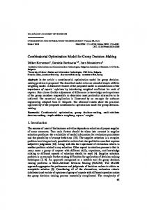
1
Fig. 1. Graph with vertex weights for the MISP. r 0
x1 x2
4
0
x3
0
2
x4 x5
0
r 3 0 0
2
0 7 0 t
(a)
0
0
r 3
0 4 0
2
0
0
0
0
0
2
2
0
0 0
0
0
7 0
3
0
2
7
0 t
(b)
0
0 t
0
(c)
Fig. 2. Representing/approximating independent sets of the graph in Figure 1 with an exact BDD (a), relaxed BDD (b), and restricted BDD (c). Each layer in a BDD corresponds to binary decision xi , where a dashed arc represents excluding vertex i, and a solid arc represents including vertex i.
in B, then the family of subsets of V represented by B is given by Sol(B) = ∪p∈P(B) V (p). B is exact for G if Sol(B) = I(G) and is relaxed (resp. restricted ) if Sol(B) ⊇ I(G)(resp.Sol(B) ⊆ I(G)). The weight w(p) of a pathPp ∈ P(B) corresponds to the weight of the subset represented by p: w(p) = a∈p w(a). We therefore have that the maximum path weight in B, z ∗ (B), equals the size of the maximum weight set in Sol(B). When B is exact, z ∗ (B) = v ∗ (G), and when B is relaxed, resp. restricted, z ∗ (B) ≥ v ∗ (G), resp.z ∗ (B) ≤ v ∗ (G). ˜ ˜ To each r − u path p we associate a path-state E(p) ⊆ V . E(p) represents the set of vertices of V which correspond to the layers below node u that are not ˜ adjacent to any vertex in V (p); i.e., E(p) := {i ≥ ℓ(u) | ∀ j ∈ V (p) : (j, i) ∈ / E}. Path-states induce a state for each node u defined by the union of all path˜ states ending at u: i.e., E(u) := ∪p∈P(B|r,u ) E(p). Note that in an exact BDD, ˜ ˜ E(p1 ) = E(p2 ) for p1 , p2 ∈ P(B|r,u ). An example of an exact, relaxed, and restricted BDD for the graph in Figure 1 is given in Figure 2. The longest path length in the exact BDD (left-most diagram) is 11 and corresponds to vertex set {2, 5}. The longest path in the relaxed BDD (middle diagram) is 13, an upper bound on the optimal value, while the longest path value in the restricted BDD (right diagram) is 9, a lower bound on the objective value, and corresponds to vertex set {3, 5}.
2.2
BDD Construction
One technique for building BDDs is by top-down construction, which starts at the root node r, assigns the root state E(r) = V , and then creates the BDD layer-by-layer. Having constructed all nodes with ℓ(u) ≤ j, the algorithm builds layer j + 1 by examining the nodes with ℓ(u) = j. If j ∈ / E(u), ℓ(u) is increased by 1, pushing it to the next layer j + 1. Otherwise, two nodes u0 , u1 with ℓ(u0 ) = ℓ(u1 ) = j + 1 are created along with arcs ak = (u, uk ), d(ak ) = k for k = 0, 1. E(u0 ) = E(u)\{j} and E(u1 ) = E(u)\ ({j} ∪ N (j)). If two nodes w1 , w2 are created for which E(w1 ) = E(w2 ), they are merged by creating node w and redirected all arcs with tail w1 or w2 to w, deleting w1 and w2 . It has been shown [8] that the algorithm described above generates an exact BDD for the MISP, and that the states established by running the algorithm are equivalent to the definition of the state in the previous subsection. If an exact BDD can be constructed, it will exactly represent the family of independent sets, and therefore allow us to find the optimal value for the MISP by a single longest-path calculation. However, for most practically-sized problems, the BDD will grow exponentially large, requiring a modification of the algorithm that will create a relaxed/restricted BDD, from which we can extract upper/lower bounds, respectively, as described in the previous subsection. To create a relaxed BDD, we forcibly merge nodes after each layer j is created if the number of nodes with ℓ(u) = j + 1 exceeds a pre-set maximum allotted width W . We reassign the state of the node as the union of the states of the nodes that are merged, and continue the construction algorithm as before, merging nodes whenever the width exceeds W . This process creates a relaxed BDD [10]. To create a restricted BDD, if the number of nodes with ℓ(u) = j + 1 exceeds W , we choose some nodes and delete them until the number of nodes in the layer equals W ; see Bergman et al. [9]. This will ensure that a restricted BDD is created since we are never modifying any states – simply deleting nodes, and hence paths. 2.3
The Branch-and-Bound Algorithm
The branch-and-bound algorithm proceeds by branching on nodes in relaxed BDDs. Before describing the algorithm, we first define, recursively, exact versus relaxed nodes in relaxed BDDs. The root r is exact, and any other node u in a relaxed BDD B is exact if all nodes u′ with arcs (u′ , u) directed to u are exact, ˜ and E(p) = E(u), for all p ∈ P(B|r,u ). A node is relaxed otherwise. An exact cut C is a set of exact nodes whose removal disconnects r and t. The following theorem by Bergman [5] provides the basis for the algorithm: Theorem 1 ([5]). Let B be a relaxed BDD for a graph G and let C be an exact cut of B. Then, v ∗ (G) = max {z ∗ (B|r,u ) + v ∗ (G[E(u)])} . u∈C
Theorem 1 thereby establishes that, having constructed a relaxed BDD for G, we can branch on any exact cut C, and solve the problem defined by the graphs G[E(u)] for every u ∈ C, adding the longest path to the nodes u to find the optimal value. Note that each node in the exact cut can therefore be processed individually by recording only the state of the node and the longest-path value up to that node in the relaxed BDD that created the node. In general there are many choices for an exact cut to branch on. One possible cut is any layer prior to the first forced node merger during the top-down construction. Let ℓ˜ be the first layer where we forcibly merged nodes together ˜ each node must be exact, and during the relaxation construction. For any j < ℓ, any such layer (which contains all nodes with ℓ(u) = j) will be an exact cut and can be used to create subproblems. Another possible cut is the frontier cut [5]. The algorithm branches on a set of partial solutions, as opposed to individual assignments of values to the problem variables, as is typically seen in algorithms designed to solve discrete optimization problems. This removes symmetry, and also allows the subproblems to be solved recursively, and individually. In principle, each node defines a subproblem which can be solved by any technique, but for the purpose of this paper, we will build restricted BDDs for primal heuristics, and relaxed BDDs for relaxation bounds, recursively defining subproblems.
3
Parallelizing BDD-Based Branch-and-Bound
The limited amount of information required for each BDD node makes the branch-and-bound algorithm naturally suitable for parallel processing. Once an exact cut C is computed for a relaxed BDD, the nodes u ∈ C are independent and can be each processed in parallel. The information required to process a node u ∈ C is its corresponding state, which is bounded by the number of vertices of G, |V |. After processing a node u, only the lower bound v ∗ (G[E(u)]) is needed to compute the optimal value, as shown in Theorem 1. 3.1
A Centralized Parallelization Scheme
There are many possible parallel strategies that can exploit this natural characteristic of the branch-and-bound algorithm for approximate decision diagrams. We propose here a centralized strategy defined as follows. A master process keeps a pool of BDD nodes to be processed, first initialized with a single node associated with the root state V . The master distributes the BDD nodes to a set of workers. Each worker receives a number of nodes, processes them by creating the corresponding relaxed and restricted BDDs, and either sends back to the master new nodes to explore (from an exact cut of their relaxed BDD) or sends to the master as well as all workers an improved lower bound from a restricted BDD. The workers also send the upper bound obtained from the relaxed BDD from which the nodes were extracted, which is then used by the master for potentially pruning the nodes according to the current best lower bound at the time these nodes are brought out from the global pool to be processed.
Even though conceptually simple, our centralized parallelization strategy involves communication between all workers and many choices that have a significant impact on performance. After discussing the challenge of effective parallelization, we explore some of these choices in the rest of this section. 3.2
The Challenge of Effective Parallelization
Clearly, a BDD constructed in parallel as described above can be very different in structure and overall size from a BDD constructed sequentially for the same problem instance. As a simple example, consider two nodes u1 and u2 in the exact cut C. By processing u1 first, one could potentially improve the lower bound so much that u2 can be pruned right away in the sequential case. In the parallel setting, however, while worker 1 processes u1 , worker 2 will be already wasting search effort on u2 , not knowing that u2 could simply be pruned if it waited for worker 1 to finish processing u1 . In general, the order in which nodes are processed in the approximate BDD matters — information passed on by nodes processed earlier can substantially alter the direction of search later. This is very clear in the context of combinatorial search for SAT, where dynamic variable activities and clauses learned from conflicts dramatically alter the behavior of subsequent search. Similarly, bounds in MIP and impacts in CP influence subsequent search. Issues of this nature pose a challenge to effective parallelization of anything but brute force combinatorial search oblivious to the order in which the search space is explored. Such a search is, of course, trivial to parallelize. For most search methods of interest, however, a parallelization strategy that delicately balances independence of workers with timely sharing of information is often the key to success. As our experiments will demonstrate, our implementation, DDX10, achieves this balance to a large extent on both random and structured instances of the independent set problem. In particular, the overall size of parallel BDDs is not much larger than that of the corresponding sequential BDDs. In the remainder of this section, we discuss the various aspects of DDX10 that contribute to this desirable behavior. 3.3
Global and Local Pools
We refer to the pool of nodes kept by the master as the global pool. Each node in the global pool has two pieces of information: a state, which is necessary to build the relaxed and restricted BDDs, and the longest path value in the relaxed BDD that created that node, from the root to the node. All nodes sent to the master are first stored in the global pool and are then redistributed to the workers. Nodes with an upper bound that is no more than the best found lower bound at the time are pruned from the pool, as these can never provide a solution better than one already found. In order to select which nodes to send to workers first, the global pool is implemented here using a data structure that mixes a priority queue and a stack. Initially, the global pool gives priority to nodes that have a larger upper
bound, which intuitively are nodes with higher potential to yield better solutions. However, this search strategy simulates a best-first search and may result in an exponential number of nodes in the global queue that still need to be explored. To remedy this, the global pool switches to a last-in, first-out node selection strategy when its size reaches a particular value (denoted maxPQueueLength), adjusted according to the available memory on the machine where the master runs. This strategy resembles a stack-based depth-first search and limits the total amount of memory necessary to perform search. Besides the global pool, workers also keep a local pool of nodes. The subproblems represented by the nodes are usually small, making it advantageous for workers to keep their own pool so as to reduce the overall communication to the master. The local pool is represented by a priority queue, selecting nodes with a larger upper bound first. After a relaxed BDD is created, a certain fraction of the nodes (with preference to those with a larger upper bound) in the exact cut is sent to the master, while the remaining fraction (denoted fracToKeep) of nodes are added to the local pool. The local pool size is also limited; when the pool reaches this maximum size (denoted maxLocalPoolSize), we stop adding more nodes to the local queue and start sending any newly created nodes directly to the master. When a worker’s local pool becomes empty, it notifies the master that it is ready to receive new nodes. 3.4
Load Balancing
The global queue starts off with a single node corresponding to the root state V , which is assigned to an arbitrary worker which then applies a cut to produce more states and sends a fraction of them, as discussed above, back to the global queue. The size of the global pool thus starts to grow rapidly and one must choose how many nodes to send subsequently to other workers. Sending one node (the one with the highest priority) to a worker at a time would mimic the sequential case most closely. However, it would also result in the most number of communications between the master and the workers, which often results in a prohibitively large system overhead. On the other hand, sending too many nodes at once to a single worker runs the risk of starvation, i.e., the global queue becoming empty and other workers sitting idle waiting to receive new work. Based on experimentation with representative instances, we propose the following parameterized scheme to dynamically decide how many nodes the master should send to a worker at any time. Here, we use the notation [x]uℓ as a shorthand for min{u, max{ℓ, x}}, that is, x capped to lie in the interval [ℓ, u]. h n q oi∞ (1) nNodesToSend c,¯c,c∗ (s, q, w) = min c¯s, c∗ w c where s is a decaying running average of the number of nodes added to the global pool by workers after processing a node,4 q is the current size of the global pool, w is the number of workers, and c, c¯, and c∗ are parametrization constants. 4
When a cut C is applied upon processing a node, the value of s is updated as snew = rsold + (1 − r)|C|, with r = 0.5 in the current implementation.
The intuition behind this choice is as follows. c is a flat lower limit (a relatively small number) on how many nodes are sent at a time irrespective of other factors. The inner minimum expression upper bounds the number of nodes to send to be no more than both (a constant times) the number of nodes the worker is in turn expected to return to the global queue upon processing each node and (a constant times) an even division of all current nodes in the queue into the number of workers. The first influences how fast the global queue grows while the second relates to fairness among workers and the possibility of starvation. Larger values of c, c¯, and c∗ reduce the number of times communication occurs between the master and workers, at the expense of moving further away from mimicking the sequential case. Load balancing also involves appropriately setting the fracToKeep value discussed earlier. We use the following scheme, parameterized by d and d∗ : 1
fracToKeep d,d∗ (t) = [t/d∗ ]d
(2)
where t is the number of states received by the worker. In other words, the fraction of nodes to keep for the local queue is 1/d∗ times the number of states received by the worker, capped to lie in the range [d, 1]. 3.5
DDX10: Implementing Parallelization Using X10
As mentioned earlier, X10 is a high-level parallel programming and execution framework. It supports parallelism natively and applications built with it can be compiled to run on various operating systems and communication hardware. Similar to SatX10 [11], we capitalize on the fact that X10 can incorporate existing libraries written in C++ or Java. We start off with the sequential version of the BDD code base for MISP [7] and integrate it in X10, using the C++ backend. The integration involves adding hooks to the BDD class so that (a) the master can communicate a set of starting nodes to build approximate BDDs for, (b) each worker can communicate nodes (and corresponding upper bounds) of an exact cut back to the master, and (c) each worker can send updated lower bounds immediately to all other workers and the master so as to enable pruning. The global pool for the master is implemented natively in X10 using a simple combination of a priority queue and a stack. The DDX10 framework itself (consisting mainly of the main DDSolver class in DDX10.x10 and the pool in StatePool.x10) is generic and not tied to MISP in any way. It can, in principle, work with any maximization or minimization problem for which states for a BDD (or even an MDD) can be appropriately defined.
4
Experimental Results
The MISP problem can be formulated and solved using several existing general purpose discrete optimization techniques. A MIP formulation is considered to be very effective and has been used previously to evaluate the sequential BDD
approach [7]. Given the availability of parallel MIP solvers as a comparison point, we present two sets of experiments on the MISP problem: (1) we compare DDX10 with a MIP formulation solved using IBM ILOG CPLEX 12.5.1 on up to 32 cores, and (2) we show how DDX10 scales when going beyond 32 cores and employing up to 256 cores distributed across a cluster. We borrow the MIP encoding from Bergman et al. [7] and employ the built-in parallel branchand-bound MIP search mechanism of CPLEX. The comparison with CPLEX is limited to 32 cores because this is the largest number of cores we have available on a single machine (note that CPLEX 12.5.1 does not support distributed execution). Since the current version of DDX10 is not deterministic, we run CPLEX also in its non-deterministic (‘opportunistic’) mode. DDX10 is implemented using X10 2.3.1 [28] and compiled using the C++ backend with g++ 4.4.5.5 For all experiments with DDX10, we used the following values of the parameters of the parallelization scheme as discussed in Section 3: maxPQueueLength = 5.5 × 10⁹ (determined based on the available memory on the machine storing the global queue), maxLocalPoolSize = 1000, c = 10, c¯ = 1.0, c∗ = 2.0, d = 0.1 and d∗ = 100. The maximum width W for the BDD generated at each subproblem was set to be the number of free variables (i.e., the number of active vertices) in the state of the BDD node that generated the subproblem. The type of exact cut used in the branch-and-bound algorithm for the experiments was the frontier cut [5]. These values and parameters were chosen based on experimentation on our cluster with a few representative instances, keeping in mind their overall impact on load balancing and pruning as discussed earlier. 4.1
DDX10 versus Parallel MIP
The comparison between DDX10 and IBM ILOG CPLEX 12.5.1 was conducted on 2.3 GHz AMD Opteron 6134 machines with 32 cores, 64 GB RAM, 512 KB L2 cache, and 12 MB L3 cache. To draw meaningful conclusions about the scaling behavior of CPLEX vs. DDX10 as the number w of workers is increased, we start by selecting problem instances where both approaches exhibit comparable performance in the sequential setting. To this end, we generated random MISP instances as also used previously by Bergman et al. [7]. We report comparison on instances with 170 vertices and six graph densities ρ = 0.19, 0.21, 0.23, 0.25, 0.27, and 0.29. For each ρ, we generated five random graphs, obtaining a total of 30 problem instances. For each pair (ρ, w) with w being the number of workers, we aggregate the runtime over the five random graphs using the geometric mean. Figure 3 summarizes the result of this comparison for w = 1, 2, 4, 16, and 32. As we see, CPLEX and DDX10 display comparable performance for w = 1 (the left-most data points). While the performance of CPLEX varies relatively little as a function of the graph density ρ, that of DDX10 varies more widely. 5
The current version of DDX10 may be downloaded from http://www.andrew.cmu. edu/user/vanhoeve/mdd
D19 D21 D23 D25 D27 D29
100
D19 D21 D23 D25 D27 D29
1000
Time (seconds)
Time (seconds)
1000
10
100
10
1
1 1
10
1
Number of Cores
10 Number of Cores
Fig. 3. Performance of CPLEX (left) and DDX10 (right), with one curve for each graph density ρ shown in the legend as a percentage. Both runtime (y-axis) and number of cores (x-axis) are in log-scale. D19 D21 D23 D25 D27 D29
100
10
D19 D21 D23 D25 D27 D29
1000
Time (seconds)
Time (seconds)
1000
100
10
1
1 1
10 Number of Cores
100
1
10 Number of Cores
100
Fig. 4. Scaling behavior of DDX10 on MISP instances with 170 (left) and 190 (right) vertices, with one curve for each graph density ρ shown in the legend as a percentage. Both runtime (y-axis) and number of cores (x-axis) are in log-scale.
As observed earlier by Bergman et al. [7] for the sequential case, BDD-based branch-and-bound performs better on higher density graphs than sparse graphs. Nevertheless, the performance of the two approaches when w = 1 is in a comparable range for the observation we want to make, which is the following: DDX10 scales more consistently than CPLEX when invoked in parallel and also retains its advantage on higher density graphs. For ρ > 0.23, DDX10 is clearly exploiting parallelism better than CPLEX. For example, for ρ = 0.29 and w = 1, DDX10 takes about 80 seconds to solve the instances while CPLEX needs about 100 seconds—a modest performance ratio of 1.25. This same performance ratio increases to 5.5 when both methods use w = 32 workers. 4.2
Parallel versus Sequential Decision Diagrams
The two experiments reported in this section were conducted on a larger cluster, with 13 of 3.8 GHz Power7 machines (CHRP IBM 9125-F2C) with 32 cores (4way SMT for 128 hardware threads) and 128 GB of RAM. The machines are
Table 1. Runtime (seconds) of DDX10 on DIMACS instances. Timeout = 1800. instance hamming8-4.clq brock200 4.clq san400 0.7 1.clq p hat300-2.clq san1000.clq p hat1000-1.clq sanr400 0.5.clq san200 0.9 2.clq sanr200 0.7.clq san400 0.7 2.clq p hat1500-1.clq brock200 1.clq hamming8-2.clq gen200 p0.9 55.clq C125.9.clq san400 0.7 3.clq p hat500-2.clq p hat300-3.clq san400 0.9 1.clq san200 0.9 3.clq gen200 p0.9 44.clq sanr400 0.7.clq p hat700-2.clq
n density 256 200 400 300 1000 1000 400 200 200 400 1500 200 256 200 125 400 500 300 400 200 200 400 700
1 core 4 cores 16 cores 64 cores 256 cores
0.36 25.24 0.34 33.43 0.30 33.96 0.51 34.36 0.50 40.02 0.76 43.35 0.50 77.30 0.10 93.40 0.30 117.66 0.30 234.54 0.75 379.63 0.25 586.26 0.03 663.88 0.10 717.64 0.10 1100.91 0.30 – 0.50 – 0.26 – 0.10 – 0.10 – 0.10 – 0.30 – 0.50 –
7.08 9.04 9.43 9.17 12.06 12.10 18.10 23.72 30.21 59.34 100.3 150.3 166.49 143.90 277.07 709.03 736.39 – – – – – –
2.33 2.84 4.63 2.74 7.15 4.47 5.61 7.68 8.26 16.03 29.09 39.95 41.80 43.83 70.74 184.84 193.55 1158.18 1386.42 – – – –
1.32 1.45 1.77 1.69 2.15 2.84 2.18 3.64 2.52 6.05 10.62 12.74 23.18 12.30 19.53 54.62 62.06 349.75 345.66 487.11 1713.76 – –
0.68 1.03 0.80 0.79 9.09 1.66 2.16 1.65 2.08 4.28 25.18 6.55 14.38 6.13 8.07 136.47 23.81 172.34 125.27 170.08 682.28 1366.98 1405.46
connected via a network that supports the PAMI message passing interface [21], although DDX10 can also be easily compiled to run using the usual network communication with TCP sockets. We used 24 workers on each machine, using as many machines as necessary to operate w workers in parallel.
Random Instances. The first experiment reuses the random MISP instances introduced in the previous section, with the addition of similar but harder instances on graphs with 190 vertices, resulting in 60 instances in total. As Figure 4 shows, DDX10 scales near-linearly up to 64 cores and still very well up to 256 cores. The slight degradation in performance when going to 256 cores is more apparent for the higher density instances (lower curves in the plots), which do not have much room left for linear speedups as they need only a couple of seconds to be solved with 64 cores. For the harder instances (upper curves), the scaling is still satisfactory even if not linear. As noted earlier, coming anywhere close to near-linear speedups for complex combinatorial search and optimization methods has been remarkably hard for SAT and MIP. These results show that parallelization of BDD based branch-and-bound can be much more effective.
Table 2. Number of nodes in multiples of 1, 000 processed (#No) and pruned (#Pr) by DDX10 as a function of the number of cores. Same setup as in Table 1.
instance
1 core 4 cores #No #Pr #No #Pr
hamming8-4.clq 43 110 brock200 4.clq san400 0.7 1.clq 7 p hat300-2.clq 80 san1000.clq 29 p hat1000-1.clq 225 451 sanr400 0.5.clq san200 0.9 2.clq 22 sanr200 0.7.clq 260 98 san400 0.7 2.clq p hat1500-1.clq 1586 brock200 1.clq 1378 hamming8-2.clq 45 gen200 p0.9 55.clq 287 C125.9.clq 1066 san400 0.7 3.clq – p hat500-2.clq – – p hat300-3.clq san400 0.9 1.clq – san200 0.9 3.clq – – gen200 p0.9 44.clq sanr400 0.7.clq – p hat700-2.clq –
0 42 1 31 16 8 153 0 3 2 380 384 0 88 2 – – – – – – – –
42 112 8 74 50 209 252 20 259 99 1587 1389 49 180 1068 2975 2896 – – – – – –
16 cores #No #Pr
64 cores #No #Pr
256 cores #No #Pr
0 40 0 32 0 41 0 45 100 37 83 30 71 25 1 6 0 10 1 14 1 27 45 11 46 7 65 12 37 18 4 13 6 28 6 0 154 1 163 1 206 1 5 354 83 187 7 206 5 0 19 0 18 1 25 0 5 271 17 218 4 193 6 5 112 21 147 67 101 35 392 1511 402 962 224 1028 13 393 1396 403 1321 393 998 249 0 49 0 47 0 80 0 6 286 90 213 58 217 71 0 1104 38 1052 13 959 19 913 2969 916 2789 779 1761 42 710 3011 861 3635 1442 2243 342 – 18032 4190 17638 3867 15852 2881 – 2288 238 2218 207 2338 422 – – – 9796 390 10302 872 – – – 43898 5148 45761 7446 – – – – – 135029 247 – – – – – 89845 8054
DIMACS Instances. The second experiment is on the DIMACS instances used by Bergman [5] and Bergman et al. [7], where it was demonstrated that sequential BDD-based branch-and-bound has complementary strengths compared to sequential CPLEX and outperforms the latter on several instances, often the ones with higher graph density ρ. We consider here the subset of instances that take at least 10 seconds (on our machines) to solve using sequential BDDs and omit any that cannot be solved within the time limit of 1800 seconds (even with 256 cores). The performance of DDX10 with w = 1, 4, 16, 64, and 256 is reported in Table 1, with rows sorted by hardness of instances. These instances represent a wide range of graph size, density, and structure. As we see from the table, DDX10 is able to scale very well to 256 cores. Except for three instances, it is significantly faster on 256 cores than on 64 cores, despite the substantially larger communication overhead for workload distribution and bound sharing. Table 2 reports the total number of nodes processed through the global queue, as well as the number of nodes pruned due to bounds communicated by the work-
ers.6 Somewhat surprisingly, the number of nodes processed does not increase by much compared to the sequential case, despite the fact that hundreds of workers start processing nodes in parallel without waiting for potentially improved bounds which might have been obtained by processing nodes sequentially. Furthermore, the number of pruned nodes also stays steady as w grows, indicating that bounds communication is working effectively. This provides insight into the amiable scaling behavior of DDX10 and shows that it is able to retain sufficient global knowledge even when executed in a distributed fashion.
5
Summary and Future Work
We have introduced a parallelization scheme for a branch-and-bound search based on approximate binary decision diagrams. We implemented our approach using the X10 parallel programming and execution framework. Our application of the technique to the maximum independent set problem demonstrates that approximate BDD-based branch-and-bound can scale significantly better with increasing number of workers than a state-of-the-art commercial-strength solver. The results indicate that the solution technique is amenable to effective parallelization on hundreds of compute cores. Besides extending DDX10 to different problem classes in addition to MISP, two interesting extensions of the underlying parallel framework would be to support determinism and decentralized load balancing. Determinism is important to many industrial users and therefore a desirable feature. Conveniently, X10 comes with native determinacy constructs called clocks that can be employed in order to ensure that DDX10 can also be executed deterministically. Second, while the centralized load balancing scheme proposed here scaled well to 256 cores, a central global queue is likely to become a bottleneck when extending to thousands of cores. Particularly attractive in the current setting is the recent work by Saraswat et al. [27] which provides a general determinate application framework, called the Global Load-Balancing (GLB) framework, available as a library in the latest release of X10. The GLB framework is responsible for automatically distributing the generated collection of tasks across all nodes, and detecting global termination. This can be used to design a distributed variant of DDX10 targeted for much larger compute clusters. In summary, our work highlights how integrating branch-and-bound based on approximate decision diagrams into X10 allows one to leverage the features of a major parallel programming language in order to substantially improve our ability to solve hard combinatorial optimization problems by exploiting hundreds of compute cores in parallel. 6
Here we do not take into account the number of nodes added to local pools, which is usually a small fraction of the number of nodes processed by the global pool.
Bibliography [1] S. B. Akers. Binary decision diagrams. IEEE Transactions on Computers, C-27: 509–516, 1978. [2] H. Andersen, T. Hadzic, J. Hooker, and P. Tiedemann. A Constraint Store Based on Multivalued Decision Diagrams. In Proceedings of the 13th International Conference on Principles and Practice of Constraint Programming (CP), vol. 4741 of Lecture Notes in Computer Science, pp. 118–132. Springer, 2007. [3] B. Balasundaram, S. Butenko, and I. V. Hicks. Clique relaxations in social network analysis: The maximum k-plex problem. Operations Research, 59(1):133–142, Jan. 2011. [4] M. Behle. Binary Decision Diagrams and Integer Programming. PhD thesis, Max Planck Institute for Computer Science, 2007. [5] D. Bergman. New Techniques for Discrete Optimization. PhD thesis, Tepper School of Business, Carnegie Mellon University, 2013. [6] D. Bergman, A. A. Cire, and W.-J. van Hoeve. MDD Propagation for Sequence Constraints. JAIR, to appear. [7] D. Bergman, A. A. Cire, W.-J. van Hoeve, and J. N. Hooker. Discrete optimization with decision diagrams, 2013. Under review. [8] D. Bergman, A. A. Cire, W.-J. van Hoeve, and J. N. Hooker. Optimization bounds from binary decision diagrams. INFORMS Journal on Computing, to appear. [9] D. Bergman, A. A. Cire, W.-J. van Hoeve, and T. Yunes. BDD-based heuristics for binary optimization. Journal of Heuristics, to appear. [10] D. Bergman, W.-J. van Hoeve, and J. N. Hooker. Manipulating MDD relaxations for combinatorial optimization. In Proceedings of CPAIOR, vol. 6697 of LNCS, pp. 20–35, 2011. [11] B. Bloom, D. Grove, B. Herta, A. Sabharwal, H. Samulowitz, and V. Saraswat. SatX10: A scalable plug & play parallel SAT framework. In Proceedings of SAT, vol. 7317 of LNCS, pp. 463–468. Springer, 2012. [12] R. E. Bryant. Graph-based algorithms for boolean function manipulation. IEEE Transactions on Computers, C-35:677–691, 1986. [13] P. Charles, C. Grothoff, V. Saraswat, C. Donawa, A. Kielstra, K. Ebcioglu, C. von Praun, and V. Sarkar. X10: an object-oriented approach to non-uniform cluster computing. In OOPSLA ’05, pp. 519–538, San Diego, CA, USA, 2005. [14] G. Chu, C. Schulte, and P. J. Stuckey. Confidence-Based Work Stealing in Parallel Constraint Programming. In Proceedings of CP, pp. 226–241, 2009. [15] A. A. Cire and W.-J. van Hoeve. Multivalued decision diagrams for sequencing problems. Operations Research, 61(6):1411–1428, 2013. [16] J. D. Eblen, C. A. Phillips, G. L. Rogers, and M. A. Langston. The maximum clique enumeration problem: Algorithms, applications and implementations. In Proceedings of the 7th international conference on Bioinformatics research and applications, ISBRA’11, pp. 306–319, Berlin, Heidelberg, 2011. Springer-Verlag. [17] J. Edachery, A. Sen, and F. J. Brandenburg. Graph clustering using distance-k cliques. In Proceedings of Graph Drawing, vol. 1731 of LNCS, pp. 98–106. SpringerVerlag, 1999. [18] Z. Gu. Gurobi Optimization - Gurobi Compute Server, Distributed Tuning Tool and Distributed Concurrent MIP Solver. In INFORMS Annual Meeting, 2013. See also http://www.gurobi.com/products/gurobi-computeserver/distributed-optimization.
[19] S. Hoda, W.-J. v. Hoeve, and J. N. Hooker. A systematic approach to MDD-based constraint programming. In Proceedings of the 16th International Conference on Principles and Practices of Constraint Programming (CP 2010), vol. 6308 of Lecture Notes in Computer Science, pp. 266–280. Springer, 2010. [20] M. J¨ arvisalo, D. Le Berre, O. Roussel, and L. Simon. The international SAT solver competitions. Artificial Intelligence Magazine (AI Magazine), 1(33):89–94, 2012. [21] S. Kumar, A. R. Mamidala, D. Faraj, B. Smith, M. Blocksome, B. Cernohous, D. Miller, J. Parker, J. Ratterman, P. Heidelberger, D. Chen, and B. SteinmacherBurrow. PAMI: A parallel active message interface for the Blue Gene/Q supercomputer. In IPDPS-2012: 26th IEEE International Parallel & Distributed Processing Symposium, pp. 763–773, 2012. [22] C. Y. Lee. Representation of switching circuits by binary-decision programs. Bell Systems Technical Journal, 38:985–999, 1959. [23] T. Moisan, J. Gaudreault, and C.-G. Quimper. Parallel Discrepancy-Based Search. In Proceedings of CP, pp. 30–46, 2013. [24] L. Perron. Search Procedures and Parallelism in Constraint Programming. In Proceedings of CP, pp. 346–360, 1999. [25] J.-C. R´egin, M. Rezgui, and A. Malapert. Embarrasingly Parallel Search. In Proceedings of CP, vol. 8124 of LNCS, pp. 596–610, 2013. [26] V. Saraswat, B. Bloom, I. Peshansky, O. Tardieu, and D. Grove. Report on the experimental language, X10. Technical report, IBM Research, 2011. [27] V. A. Saraswat, P. Kambadur, S. Kodali, D. Grove, and S. Krishnamoorthy. Lifeline-based global load balancing. In Proceedings of the 16th ACM Symposium on Principles and Practice of Parallel Programming, PPoPP ’11, pp. 201–212, New York, NY, USA, 2011. ACM. ISBN 978-1-4503-0119-0. URL http://doi.acm.org/10.1145/1941553.1941582. [28] X10. X10 programming language web site. http://x10-lang.org/, Jan. 2010.