Parallel Computation of Multidimensional Polynomials in State ...

Parallel Computation of Multidimensional Polynomials in State Equation of Seawater J. Mendez Institute of Intelligent Systems(SIANI), Univ. Las Palmas de Gran Canaria 35017 Las Palmas, Canary Islands, Spain, Email: [email protected] Abstract— The computation of the standard formulation of the International Association for the Properties of Water and Steam for seawater requires the evaluation of some multidimensional polynomials to obtain the thermodynamical properties useful in industrial processes as desalination and in the massive simulation of the oceans. These polynomials are related to the Gibbs free energy function and its first and second derivatives. A computational model to parallelize the evaluation of those polynomials is proposed by using both vector and multicore parallelization. In the implementations carried out, the combined performance of both paradigms generates significant speed-up. The interest of this paper for the general scientific community lies in the fact that future simulations that achieve the exact model of that standard for seawater will require efficient programming of these equations. Keywords: Gibbs Free Energy; Seawater Properties; Polynomial Evaluation; Parallel Computation; SIMD; Multicore Systems

1. Introduction The International Association for the Properties of Water and Steam (IAPWS) has recently formulated its state equation for the seawater based on the formulation of the Gibbs free energy as a multidimensional polynomial[1]. The properties of seawater are interesting in industrial applications, such as in desalination processes, but the massive computation of seawater properties is mainly required in oceanographic simulations. Seawater is the main matter in oceanography and oceans are the main piece of the EarthŠs climate. Therefore the computation of the thermodynamical properties of seawater is of potential interest for research of the oceans and climate. Prior to the standard formulation for the seawater, the IAPWS had been involved in the definition of the standard formulation for the ordinary water for general scientific applications[2], which we will call the Release 95, and the simplified version for water and steam formulation in industrial applications IF97[3]. The later is commonly used in Thermodynamical packages and in applications in Chemical and Energetic Engineering. The Release 95 is more complex to implement, while the IF97 is simpler to implement in the double precision supported by the hardware of most computers. The precision of the IF97 is lower than

that of Release 95 but sufficient for industrial and practical applications involving water and steam. One of the advantages of the IAPWS formulations is that they are based on the formulation of the Gibbs free energy, in that all the required thermodynamical data, e.g. enthalpy, entropy or specific head, are computed by means of polynomials in constrained areas of the state space. These polynomials are two dimensional mainly depending on the state variables: pressure, p, and temperature, T . For example, in the Region 1 of the ordinary water, which corresponds to the liquid state, the Gibb free energy g(p, T ) is computed as: 34

g(p, T ) X = ni (7.1 − π)Ii (τ − 1.222)Ji RT i=1

(1)

where π = p/p∗ and τ = T ∗ /T , and p∗ and T ∗ are constants. The coefficient ni and the exponents Ii and Ji are provided by the IAWPS formulation[3]. The computation of the thermodynamical properties is performed by computing the first and second derivatives of this polynomial on p and T . There are many packages and high quality implementations to compute the properties of ordinary water based on the IAPWS Release 95 and IF97 formulations[4]. For the seawater, which we will addressed later, the formulation includes an additional variable, salinity S, therefore the computation of seawater properties requires the computation of a three dimensional polynomial. The common trends in practical computer applications are tending to adopt standards and normalization as a way to validate the results. The definition of a standard formulation to compute the properties of seawater will move much software related to oceans and climate simulation toward the implementation of such standard as a way of validation. The proposal of faster and more efficient algorithms like those proposed in this paper, should be of general interest to the scientific community in those research areas. A case of the interest of the ocean in supercomputing activities is the project Global to Regional Oceanographic Modeling (GROM) [5] of the Distributed European Infrastructure for Supercomputing Applications (DEISA). Its main objective is to build and to validate new ocean model configurations from a global to a regional scale able to simulate the main features of the thermodynamic processes in the ocean.

Climate research attaches great importance to the simulation of Polar Oceans, where the water is mainly in the states of seawater and ice [6],the ocean circulation in those oceans is driven by atmosphere-ice-ocean interaction and the modeling of that system requires procedures that capture both the thermodynamic and the dynamic processes[7]. The computation of the Gibbs function is the first part needed to compute many of the properties used in thermodynamical and general dynamic equations. For example, one parameter obtained from the Gibbs function is the sound wave speed in seawater. The sound is used by scientific instruments to measure the properties of the sea floor, the depth of the ocean, the temperature and currents. Sound speed depends on the temperature, salinity and pressure [8], the changes and gradients in temperature and salinity generate changes and refractions in the sound waves, which modifies how the sound is propagated and scattered in the marine media. If physical phenomena in oceans are related to the surface layer of currents and circulation, called the thermocline one [9], they are different form those related to the deep water below. In the ocean’s surface layer, the currents are driven by wind and tides while, in the deep ocean the main force is the density gradient related to the changes in temperature and salinity. The term thermohaline currents or circulation[10], [11] refers to the large-scale ocean circulation that is driven by global density gradients created by the differences in temperature and salt concentration. Although the density of seawater in oceans water is globally homogeneous, it can change significantly and discretely due to local changes in both temperature and salinity. Some of this changes propagate anomalies throughout the ocean[12]; in these anomalies bounds there are steep gradients of temperature and salinity. The density of seawater can be computed by means of some derivatives of the Gibbs function, thus, in the simulation of the thermohaline currents[13] the computation of the Gibbs function for seawater and its derivatives can be relevant issues. Ocean simulation are carried out by using massive Finite Element Methods (FEM) by using spatial mesh at some defined grid size[14]. In those applications the computation of the seawater of each discrete element implies the computation of many single calls for each simulation. This paper focusses on the computation of the saline part of the Gibbs function of seawater by means of parallelizing the computation of a three dimensional polynomial, which generalizes the use of two dimensional polynomial involved in the IF97 and partially in the Release 95 of ordinary water. Both the computation of polynomial and the simulation of ocean are areas closely related to parallel computation. The most widely used approach to compute one dimensional polynomial is the Horner’s rule. It is used to evaluate the general expression: y = a0 + a1 x + · · · + an xn by using recursive formulation as: y0 = an , yk = yk−1 x + an−k , that avoids the exponent computation. Horner’s rule to evaluate

one dimensional polynomials have been studied for the last few decades[15] using special hardware, such as FPGA[16], systolic processors[17], pipeline-based computation[18] or Graphics Processors Unit(GPU)[19]. However, in this paper we address the problem for computing multidimensional polynomials from a different approach without using the Horner’s rule. Modern parallel computation is related to different levels, grain sizes and paradigms: grid, cluster, multicore, Simple Instruction Multiple Data(SIMD) and GPU. The suitable level of parallelism for the computation of seawater properties depends on the levels that are occupied by the general FEM and also on the grain size of the computation of the Gibbs function. A massive FEM should exhaust the level of grid, cluster and multicore, therefore the levels where we would place it are the GPU, SIMD and partially in the multicore ones. Although is not the most common approach, the solution of FEM can be obtained much faster by using GPUs than on CPUs, but the GPUs do not support double precision computation. Some approaches have been proposed to accelerate the computation while maintaining the precison[20], [21]. This problem of the tradeoff between precision and computational speed is also addressed in the paper. A very important issue is to decide the strategy to compute the seawater properties; the options are single call or bulk computation of all the calls associated to the different finite elements in the same computer. To include the IAPWS standard in existent codes for ocean simulation, the simplest approach is to include a single call in the code procedure where the properties of an element are computed. This approach excluded that of bulk computation. In this case, the level that should be partially unused by the FEM is the vector processing oriented level or SIMD. To include the IAPWS standard in future codes, the bulk computation option must be evaluated. The levels of SIMD, GPU and multicore would be evaluated. The computation of the saline part of Gibbs function is a fine-grain task whose computation time is in the order of a few microseconds. Climate research uses massive FEM to solve the physical models in computer clusters. However, inside the cluster nodes, multicore and SIMD processing can be exploited to compute the required properties of seawater of individual elements in oceanographic simulations. This paper addresses a practical application of parallelism at the levels of multi-core systems and SIMD. The interest of this paper for the general scientific community lies in the fact that future simulations that achieve the exact model of the IAPWS for seawater will require efficient programming of these equations. The remaind of this paper is organized in sections. The first presents the standard formulation of the saline part of the Gibbs function that is computed by means of a multidimensional polynomial. The second contains the model to parallelize the computation

of the Gibbs function and its first and second derivatives. The results section presents an implementation in multicore computers. A significant speed-up is achieved by using both SIMD and multicore paradigms.

2. Polynomial Model of the State Equations According to proposal of the IAPWS[1], the Gibbs function for the seawater is computed from two additive parts: W

S

g(S, T, p) = g (T, p) + g (S, T, p)

(2)

where the first part g W (T, p) is the water one depending on the temperature, T , and the pressure, p. This part can be computed from the IAPWS water general scientific formulation[2]. The second part g S (S, T, p) is the saline part depending on the temperature, pressure and the salt concentration S. This part, which is the concern of this paper, is defined as:

S

g (S, T, p) =

5 X 6 X

à 2

g1jk ξ ln ξ +

k=0 j=0

7 X

! gijk ξ

i

τ j πk

i=2

(3) where τ = (T − T )/T , π = (p − p )/p and ξ = 0 0 p S/S ∗ . The parameters T0 , T ∗ , p0 , p∗ , and S ∗ are defined in the IAPWS report. The no null g1jk elements are g100 and g110 , therefore the saline part can be computed as: ∗

S

g (S, T, p) = f (τ, ξ) +

∗

5 X 6 X 7 X

i j k

hijk ξ τ π

(4)

k=0 j=0 i=0

The computation of f (τ, ξ) is trivial and this paper focuses in the computation of the polynomial second right term. The number of non null elements gijk is 64, the number of no null g1jk is only 2, so the number of non null elements in hijk is 62. To fit better in vector computation tasks, which run best for 2n dimension, we use hijk = gijk with the exception of h100 = h110 = 0. The first and second derivatives of the Gibbs function are needed to compute many physical and thermodynamical properties of seawater. For example, the seawater density is computed as: ρ(S, T, p) = [∂p g]−1 , and the sound speed, w(S, T, p), is computed from the first and second derivatives as: q w(S, T, p) = ∂p g

∂T T g/([∂T p g]2 − ∂T T g ∂pp g)

(5)

These derivatives are of the whole Gibbs function, which can be computed additively from the general formulation of ordinary water and the saline part. To carry out the parallelization process we introduce a generalization of the polynomial problem by abstracting that X, Y and Z are functions of the salinity, temperature and pressure, and

our problem concerns the computation of the following polynomial and its first and second derivatives: P (X, Y, Z) =

ny nz nx X X X

aijk X i Y j Z k

(6)

i=0 j=0 k=0

We use the following model based on the sparse representation of the non null values of aijk contained in the vector A[l]; l = 0, . . . , N − 1. P (X, Y, Z) =

N −1 X

A[l]X I[l] Y J[l] Z K[l]

(7)

l=0

In this case N = 64 and the vectors I[l], J[l] and K[l] are the exponents of the variables X, Y and Z respectively for each non null value of aijk . We have changed the tensorlike representation, aijk , to the programming-like one A[l]. These vector are represented as the floating-point: A, and three integer vectors: I, J and K. The computation of the first and second derivatives of P (X, Y, Z) are also needed. Some of these are the following, which can also be expressed as polynomials: N −1 X

∂X P =

l=0 N −1 X

∂XY P =

l=0 N −1 X

∂XX P =

A[l]I[l]X I[l]−1 Y J[l] Z K[l]

(8)

A[l]I[l]J[l]X I[l]−1 Y J[l]−1 Z K[l]

(9)

A[l]I[l](I[l] − 1)X I[l]−2 Y J[l] Z K[l] (10)

l=0

In effect, we must compute M polynomials, in our case M = 1 + 3 + 3 + 3 = 10, the polynomial itself, the first three derivative, the second three derivatives and the second three cross derivatives. Neither ∂ST g nor ∂SS g are used to obtain thermodynamical properties in the IAPWS report, so we can reduce the effective number to M = 8. Although a context computation can be achieved to compute only the polynomials needed in a particular case, we address the general problem of computing the 10 polynomials together.

3. Computational Model The first issue to be addressed is the related to the suitable precision for the implementations. We have performed a test related to the precision, it corresponds to the variable values: S = 0.03516504 kg kg−1 , T = 273.15K and p = 108 Pa. The quantities computed are the specific values for the saline part of the Gibbs function g, its first and second derivatives, the enthalpy h, the Helmholtz energy f , the internal energy u, the entropy s, the specific isobaric heat cp and the chemical potential µW . The correct results are displayed in the Table 8(c) of the IAPWS report[1]. Table 1 shows the results of the computation by using double

Table 1: Comparative results and error between double and simple precision Saline Part g ∂g/∂S ∂g/∂T ∂g/∂p ∂ 2 g/∂S∂p ∂ 2 g/∂T 2 ∂ 2 g/∂T ∂p ∂ 2 g/∂p2 h f u s cp µW

Double −2.60093051 × 103 −5.45861581 × 103 7.54045685 × 100 −2.29123842 × 10−5 −6.40757619 × 10−4 4.88076974 × 10−1 4.66284412 × 10−8 3.57345736 × 10−14 −4.66060630 × 103 −3.09692089 × 102 −2.36936788 × 103 −7.54045685 × 100 −1.33318225 × 102 −2.40897806 × 103

Simple −2.60093024 × 103 −5.45862625 × 103 7.54045678 × 100 −2.29123828 × 10−5 −6.40757576 × 10−4 4.88077126 × 10−1 4.66284218 × 10−8 3.57345703 × 10−14 −4.66060601 × 103 −3.09691957 × 102 −2.36936773 × 103 −7.54045678 × 100 −1.33318267 × 102 −2.40897743 × 103

precision, simple precision and the relative error between them ²r . The results for double precision corresponds exactly with the official values, while those for simple precision have some error. The combined values permit the conclusion that the error is approximately two parts per million. The tradeoff between precision and computational time must be chosen depending on the application, but if the two parts in million is a permisible error level for an application, the simple precision should be a well balanced option. To compute the M polynomials, we use the following representation for a, b, c = 0, 1, 2 constrained to the values: a + b + c ≤ 2:

Pabc (X, Y, Z) =

N −1 X

Aabc [l]X Ia [l] Y Jb [l] Z Kc [l]

(11)

l=0

where the polynomials correspond to the following meaning: P000 is the value of the original polynomial, P100 the first derivative on X, P200 the second derivative on X, P011 the second cross derivative on Y and Z and so on. The proposed algorithm for sparse multidimensional polynomial is equivalent to the computation of one dimensional polynomial by using the basic and well founded computational primitives such as the vector prefix and the dot product. The one dimensional problem can be computed from the coefficient vector A = [a0 , a1 , a2 , . . . , an ] and the vector F = [1, x, x2 , . . . , xn ] which can be computed by using the product-prefix computation on the vector: B = [1, x, x, . . . , x]. The polynomial solution is the dot product y = A · F . The problem of plus-scan or sum-prefix and its related product-prefix, is a classical problem of parallel computation widely studied [22][23], and more recently, has been implemented in GPU [19]. The proposed algorithm comprises composed of three phases: initialization, indexing,

|²r | 1.0 × 10−7 1.9 × 10−6 9.3 × 10−9 6.1 × 10−8 6.7 × 10−8 3.1 × 10−7 4.1 × 10−7 9.2 × 10−8 6.2 × 10−8 4.3 × 10−7 6.3 × 10−8 9.3 × 10−9 3.1 × 10−7 2.6 × 10−7

Unit J kg−1 J kg−1 J kg−1 K−1 −1 m3 kg −1 3 m kg −1 J kg K−2 −1 m3 kg K−1 −1 3 m kg Pa−1 J kg−1 J kg−1 J kg−1 J kg−1 K−1 J kg−1 K−1 J kg−1

which includes the product-prefix, and a generalization of the dot product.

3.1 Algorithm Initialization Some data must be computed at the initialization step. We used C++ code, therefore those initializations are performed in the code corresponding to the class constructor. From the original vectors A, I, J, K provided by the IAPWS, we must construct the following vectors: Ia , Ja and Ka for a = 0, 1, 2, where: Ia = (I − a)

Ja = (J − a)

Ka = (K − a) (12)

Also, the following vector must be computed: A000 = A, that related to the first derivative: A100 , A010 , A001 , the second cross derivative: A011 , A101 , A110 and the second derivative: A200 , A020 , A002 . They are computed as: A100 [l] = A[l]I0 [l] A200 [l] = A100 [l]I1 [l] A010 [l] = A[l]J0 [l] A020 [l] = A010 [l]J1 [l] A002 [l] = A001 [l]K1 [l]

A110 [l] = A100 [l]J0 [l] A101 [l] = A100 [l]K0 [l] A011 [l] = A010 [l]K0 [l] A001 [l] = A[l]K0 [l]

(13) (14) (15) (16) (17)

3.2 Indexing For the values X, Y, Z corresponding to a requested computation, we must construct the following vector: Fx = [1, X, X 2 , . . . , X nx ]

(18)

where nx is the maximum values of the exponent of the variable X in the polynomials. For the Y and Z variables, we must compute the matrices: Fy = [1, Y, Y 2 , . . . , Y ny ]

Table 2: 4-dot product A000 A100 A200 A011 A010 A020 A101 A001 A002 A110 X0 X1 X2 X0 X0 X0 X1 X0 X0 X1 Y0 Y0 Y0 Y1 Y1 Y2 Y0 Y0 Y0 Y1 Z0 Z0 Z0 Z1 Z0 Z0 Z1 Z1 Z2 Z0 P000 P100 P200 P011 P010 P020 P101 P001 P002 P110

Table 3: Vector product + 3-dot product

avoid those redundant operations, the arrangement in Table 3 can be used, which uses two phases and six vector buffers Ua ; a = 1, . . . , 6. In this case the basic computational primitives are vector product element-at-element, A[l] = B[l]C[l], to compute the buffer values and one 3-dot product: t=

X0 X0 Y0 X1 X1 Y1 Y0 Z0 Z0 Y1 Z1 Z1 U1 U2 U3 U4 U5 U6

N −1 X

A[l]B[l]C[l]

(21)

l=0

A000 A100 A200 A011 A010 A020 A101 A001 A002 A110 U1 U3 U3 U6 U2 U3 U5 U1 U1 U4 Z0 X1 X2 X0 Y1 Y2 Y0 Z1 Z2 Z0 P000 P100 P200 P011 P010 P020 P101 P001 P002 P110

The computational arrangement shown in Table 4 uses three phases and two sets of vector buffers, the six vectors Ua ; a = 1, . . . , 6 and the ten vectors: Va ; a = 1, . . . , 10. The last phase uses the dot product that can be implemented in high performance software by using the BLAS libreries[25]:

Table 4: Vector product + 2-dot product X0 X0 Y0 X1 X1 Y1 Y0 Z0 Z0 Y1 Z1 Z1 U1 U2 U3 U4 U5 U6

d=

A000 A100 A200 A011 A010 A020 A101 A001 A002 A110 V1 V2 V3 V4 V5 V6 V7 V8 V9 V10 P000 P100 P200 P011 P010 P020 P101 P001 P002 P110

and Fz = [1, Z, Z 2 , . . . , Z nz ] respectively. The indexing procedure requires the computation of the following vectors, for a = 1, 2, 3: Ya = Fy [Ja ]

Za = Fz [Ka ]

(19)

Those equations imply an indirection as: Xa [l] = Fx [Ia [l]]. The main drawback of this procedure is that it is uncoalescent, which means that it is hardly implemented in SIMD or GPU[24] processors.

3.3 Vector product and n-dot product The last step in computing the polynomials is the computation of the sum of products. Table 2 shows the arrangement of products to compute the polynomials. Every column is related with the computation of one polynomial, we must compute the products of the vector in all the rows and at the end compute the scalar, Pabc , in the bottom row. The following computational primitive is used to carry out this process, we call it the quad product or a 4-dot product, because it resembles the widely used concept of dot product of two vectors. q=

N −1 X

A[l]B[l]C[l]D[l]

A[l]B[l]

(22)

l=0

U1 U3 U3 U6 U2 U3 U5 U1 U1 U4 Z0 X1 X2 X0 Y1 Y2 Y0 Z1 Z2 Z0 V1 V2 V3 V4 V5 V6 V7 V8 V9 V10

Xa = Fx [Ia ]

N −1 X

(20)

l=0

By analyzing this Table, we can see that some products are repeated, e.g. those involving the product of X0 and Y0 . To

We can evaluate the theoretical computational cost of the three approaches by taking account of the products and the load/store memory operations. Each vertical block in the previous Tables is 64 elements wide, so we avoid having to multiply the cost by that factor because it is common to all the arrangements. We label the operations as L(load), S(store), L/S(laod/store) and P(product). That labeled L/S is the sum of the L and S operations. The arrangement in Table 2 needs: 10(4L+3P)= 40L+30P operations. The arrangement in Table 3 needs : 6(2L+1P+1S)= 18L/S+6P in the first step, and needs: 10(3L+2P)=30L+20P in the second step. In total it needs: 48L/S+26P. We can conclude that the second arrangement uses fewer product operations but requires more load/store memory operations. The third approach needs : 6(2L+1P+1S)= 18L/S+6P in the first step, it needs: 10(2L+1P+1S)= 30L/S+10P in the second step and needs: 10(2L+1P)= 20L/S+10P in the last step. In total it requires: 68L/S + 26P. Clearly, that last approach entails greater computation cost than the second approach even though it uses the simplest computational primitive of a dot product. From the viewpoint of theoretical complexity the second approach is the best, because in this theory the cost is the number of arithmetical and logical operations used to carry out a computational task. However, in practical programming in modern computers, the memory operations are more time consuming that that the arithmetic ones. In modern computers, the amount of, and way to access, main memory is more critical than the number-crunching. We can achieve more performance by reducing the data traffic between CPU and main memory and increasing the in-register arithmetical operations. In that practical viewpoint the first approach will be better because it uses less memory access although it repeats some products.

4 3.77 3.5 3

Speed−up

2.5 2 1.5 1 C++ Simple C++ Double SIMD Double SIMD Simple

0.5 CPU: Intel Core2 Duo 0

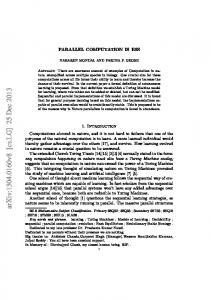
Fig. 1: In register implementation of SIMD quad product in simple precision

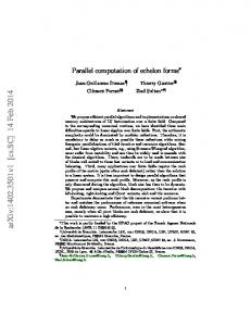
4. Results We have implemented the computation of the saline part of the Gibbs function and its first and second derivative as a C++ class. The indexing step in the algorithm is implemented in C++ source code, while the quad product is implemented both in C++, with a simple unrolled loop, and in embedded assembler by using the SIMD instructions for AMD and Intel CPUs[26]. Figure 1 shows the in-register quad product in simple precision; it uses the advantageous performance of memory referenced product to perform one load and product in the same instruction. In this implementation of the quad product, there are four partial accumulators contained in the xmm0 register; the final value requires the sum of these four values. This is an advantage because the rounding errors are lower than when using one single accumulator. To take advantage of the multicore hardware OpenMP has been used to implement a bulk computation of a million calls. The code has been compiled and run in two different computational environments. The first implementation(CPU1)is in an Intel Mobile Core2 Duo P8600, 2.40GHz, 3Mb L2 cache and 4Gb RAM. The second implementation(CPU2)is in an Intel Core2 Quad Q6600, 2.40Ghz, 2x4Mb L2 cache and 8Gb RAM. Table 5 shows the results for the CPU1 case in µs/call for a bulk computation of a million of calls for a different thread number. It includes the labels for C++ code, SIMD, double(D) and simple(S) precision. The first part of the table compares the cost of indexing vs. quad product. In this case the CPU has two cores and no additional gain is obtained after n = 2. Figure 2 shows the obtained speed-up relative to the C++ Double Precision implementation. The combined performance of SIMD and multicore generates a peak speed-up of 3.77 for the SIMD

1

2

3

4

Thread number

Fig. 2: Speed-up related to C++ double precision implementation. The combined performance of using both SIMD and multicore generate a speed-up of 3.77 for a two core CPU Table 5: Results for CPU1 µs/call vs threads

1 2 3 4

Indexing Quad Total

C(D)

C(S)

SIMD(D)

SIMD(S)

0.54 1.77 2.53

0.52 4.26 5.06

0.53 0.90 1.53

0.52 0.56 1.29

1.32 1.36 1.39

2.64 2.67 2.66

0.81 0.84 0.86

0.67 0.72 0.71

Simple Precision case at n = 2 threads. The latter has more advantage over the use of SIMD, but in pure C++ performs worse that the Double Precision implementation. In the CPU2 case, Table 6 contains the results for different number of threads. Figure 3 shows the speed-up relative to the C++ Double Precision implementation. As in the case of CPU1, the Simple Precision using SIMD has the best performance, in this case 7.44 at n = 4 threads. The combined performance of the parallelization paradigms of SIMD and multicore[27][28] is that permit this lever of speed-up. The ration of increasing of the speed-up vs number of threads is greater than 1.0 in these case since the increasing of the use of L1 cache according the number of cores involved in the computation increases. Times are measured in the main thread by using one Performance Counter that is thread safe in multicore systems. The Performance Counter has a time quantum for CPU2 of 0.4177 nsec. while for CPU1 is 0.279 µsecs. To avoid the problems related to the time granularity of single calls, which in CPU1 is close to the time quantum [29], we have compute the time for one millions of calls and reported the time corresponding to a single call.

Table 6: Results for CPU2 µs/call vs threads C(D)

C(S)

SIMD(D)

SIMD(S)

2.68 1.39 0.93 0.72 0.83 0.82 0.74 0.70 0.74

2.94 1.51 1.02 0.76 0.91 0.88 0.82 0.73 0.88

1.65 0.88 0.59 0.45 0.52 0.51 0.49 0.45 0.49

1.37 0.72 0.48 0.36 0.43 0.43 0.38 0.37 0.39

1 2 3 4 5 6 7 8 9

9 8 7,44 7

Speed−up

6 5 4 3 2 1 0

CPU: Intel Core2 Quad 1

2

3

4 5 6 Thread number

C++ Double C++ Simple SIMD Double SIMD Simple 7

8

9

Fig. 3: Speed-up related to C++ double precision implementation in CPU2. The combined performance of using both SIMD and multicore generate a speed-up of 7.44 for a four core CPU

5. Conclusion The computation of the standard formulation of IAPWS for seawater requires the evaluation of some multidimensional polynomials from which are obtained the thermodynamical properties useful in industrial processes as desalination and in the massive simulation of the oceans. A computational model to parallelize the evaluation of those polynomial that uses SIMD and multicore paradigms has been proposed. In the implementations carried out, the combined performance of both paradigms generates significant speed-up useful for the general scientific community involved in processes and simulations related to the seawater.

References [1] IAPWS, “Release on the IAPWS formulation 2008 for the thermodynamic properties of seawater,” IAPWS, Tech. Rep., 2008. [2] W. Wagner and A. Pruss, “The IAPWS formulation 1995 for the thermodynamic properties of ordinary water substance for general and scientific use,” J. Phys. Chem. Ref. Data, vol. 31, pp. 387–535, 2002. [3] W. Wagner and J. R. Cooper, “The IAPWS industrial formulation 1997 for the thermodynamic properties of water and steam,” ASME J. Eng. Gas Turbines and Power, vol. 122, pp. 150–182, 2000.

[4] W. Wagner and U. Overhoff, ThemoFluids. Springer-Verlag, 2006. [5] “Project GROM: Global to regional oceanographic modelling,” Distributed European Infrastructure for Supercomputing Applications (DEISA), Tech. Rep., 2006. [6] R. Feistel, D. G. Wright, K. Miyagawa, J. Hruby, D. R. Jackett, T. J. McDougall, and W. Wagner, “Development of thermodynamic potentials for fluid water, ice and seawater: a new standard for ˝ oceanography,” Ocean Sci. Discuss, vol. 5, pp. 375U–418, 2008. [7] R. Timmermann, A. Beckmann, and H. Hellmer, “Simulation of iceocean dynamics in the Weddell sea. part I: Model configuration and validation,” J. Geophys. Res., vol. 107, no. C3, 2002. [8] R. H. Stewart, Introduction To Physical Oceanography, 2008. [9] C. Shaji, C. Wang, G. R. Halliwell, and A. Wallcraft, “Simulation of tropical Pacific and Atlantic oceans using a hybrid coordinate ocean ˝ model,” Ocean Modelling, vol. 9, p. 253U282, 2005. [10] S. Rahmstorf, “The concept of the thermohaline circulation,” Nature, vol. 421, p. 699, 2003. [11] M. Vellinga and R. A. Wood, “Global climatic impacts of a collapse of the Atlantic thermohaline circulation,” Climatic Change, vol. 54, pp. 251 – 267, 2002. [12] M. Nonaka and H. Sasaki, “Formation mechanism for isopycnal ˝ temperatureUsalinity anomalies propagating from the eastern south pacific to the equatorial region,” Journal of Climate, vol. 20, pp. 1305– 1315, 2007. [13] V. E. Delnore, “Numerical simulation of thermohaline convection in the upper ocean,” Journal of Fluid Mechanics, vol. 96, no. 4, pp. 803–826, 1980. [14] R. D. Smith, M. E. Maltrud, F. O. Bryan, and M. W. Hecht, “Numerical simulation of the North Atlantic ocean at 1/10o ,” Journal of Physical Oceanography, vol. 30, pp. 1532 – 1561, 2000. [15] W. S. Dorn, “Generalizations of Horner’s rule for polynomial evaluation,” IBM Journal, pp. 239 – 245, April 1962. [16] A. Tisserand, “High-performance hardware operators for polynomial evaluation,” Int. J. High Performance Systems Architecture, vol. 1, no. 1, pp. 14 – 23, 2007. [17] P. Mathias and L. Patnaik, “Systolic evaluation of polynomial expressions,” IEEE Transactions on Computers, vol. 39, no. 5, pp. 653 – 665, 1990. [18] P. G. Harrison and R. L. While, “Transformation of polynomial evaluation to a pipeline via HornerŠs rule,” Science of Computer Programming, vol. 24, pp. 83 – 95, 1995. [19] M. Harris, “Parallel prefix sum(scan) with CUDA,” NVIDIA Corp., Tech. Rep., 2008. [20] D. Goddeke, R. Strzodka, and S. Turek, “Accelerating double precision FEM simulations with GPUs,” in Proceedings of ASIM 2005 18th Symposium on Simulation Technique, Sept. 2005. [21] ——, “Performance and accuracy of hardware-oriented nativeemulated and mixed-precision solvers in FEM simulations,” Int. Journal of Parallel, Emergent and Distributed Systems, 2006. [22] W. D. Hillis and J. Guy L. Steele, “Data parallel algoritms,” Communications of the ACM, vol. 29, no. 12, pp. 1170 – 1183, 1986. [23] G. E. Blelloch, “Prefix sums and their applications,” Carnegie Mellon University, Tech. Rep. CMU-CS-90-190, 1990. [24] NVIDIA CUDA. Programming Guide, NVIDIA Corporation, 2007. [25] J. Dongarra, “Basic linear algebra subprograms technical forum standard,” International Journal of High Performance Applications and Supercomputing, vol. 16, no. 2, pp. 115–199, 2002. [26] Intel 64 and IA-32 Architectures Software Developer’s Manual. Volume 2: Instruction Set Reference, Intel Corporation, November 2008. [27] H. Inoue, T. Moriyama, H. Komatsu, and T. Nakatani, “Aa-sort: A new parallel sorting algorithm for multi-core SIMD processors,” Parallel Architectures and Compilation Techniques, International Conference on, vol. 0, pp. 189–198, 2007. [28] J. Chhugani, A. D. Nguyen, V. W. Lee, W. Macy, M. Hagog, Y.-K. Chen, A. Baransi, S. Kumar, and P. Dubey, “Efficient implementation of sorting on multi-core SIMD cpu architecture,” PVLDB, vol. 1, no. 2, pp. 1313–1324, 2008. [29] W. Korn, P. J. Teller, and G. Castillo, “Just how accurate are performance counters?” in IEEE International Conference on Performance, Computing, and Communications, April 2001, pp. 303 – 310.