Parallel Computer Vision on a Reconfigurable Multiprocessor Network

292

IEEE TRANSACTIONS ON PARALLEL AND DISTRIBUTED SYSTEMS, VOL. 8, NO. 3, MARCH 1997

Parallel Computer Vision on a Reconfigurable Multiprocessor Network Suchendra M. Bhandarkar, Member, IEEE Computer Society, and Hamid R. Arabnia Abstract—A novel reconfigurable architecture based on a multiring multiprocessor network is described. The reconfigurability of the architecture is shown to result in a low network diameter and also a low degree of connectivity for each node in the network. The mathematical properties of the network topology and the hardware for the reconfiguration switch are described. Primitive parallel operations on the network topology are described and analyzed. The architecture is shown to contain 2D mesh topologies of varying sizes and also a single one-factor of the Boolean hypercube in any given configuration. A large class of algorithms for the 2D mesh and the Boolean n-cube are shown to map efficiently on the proposed architecture without loss of performance. The architecture is shown to be well suited for a number of problems in low- and intermediate-level computer vision such as the FFT, edge detection, template matching, and the Hough transform. Timing results for typical low- and intermediate-level vision algorithms on a transputerbased prototype are presented. Index Terms—Reconfigurable multiring network, reconfigurable architectures, scalable architectures, parallel processing, distributed processing, computer vision, image processing, parallel algorithms, distributed algorithms.

—————————— ✦ ——————————

1 INTRODUCTION in computer vision are known to be computationally intensive. Inherent limitations on the computational power of uniprocessor architectures, especially under real-time constraints, have led to the development of multiprocessor architectures for computer vision problems. From a theoretical point of view, a multiprocessor architecture should facilitate the design and implementation of efficient parallel algorithms for computer vision problems. These algorithms should optimally exploit the capabilities of the architecture. From an architectural point of view, the multiprocessor architecture should have low hardware complexity and, preferably, be composed of components that can be easily replicated thus making it suitable for VLSI implementation. Additionally, the architecture should exhibit good scalability of computational performance, hardware complexity, and cost with increasing number of processors. Many multiprocessor architectures have been proposed for computer vision such as, the hypercube [29], butterfly [7], systolic array [9], 2D mesh [10, [34], and the pyramid [35]. Several researchers have attempted to map computer vision problems on these architectures. However, the fixed topology of the interconnection networks describing these architectures leads to an inevitable tradeoff between the need for low network diameter and the need to limit the number of interprocessor communication links. Moreover, vision problems are especially difficult since they place different requirements on the underlying interconnection network topology and the mode or granularity of parallelism (i.e., SIMD, SPMD, or

P

ROBLEMS

————————————————

• The authors are with the Department of Computer Science, 415 Boyd Graduate Studies Research Center, the University of Georgia, Athens, GA 30602-7404. E-mail: [email protected]. Manuscript received Nov. 18, 1994. For information on obtaining reprints of this article, please send e-mail to: [email protected], and reference IEEECS Log Number D95243.

MIMD) depending on whether the problem can be classified as one of low-, intermediate-, or high-level vision. No fixed topology interconnection network with a given mode or granularity of parallelism has proven effective at tackling computer vision problems at all levels of abstraction, i.e., low-, intermediate-, and high-level vision. Reconfigurable networks attempt to address the aforementioned tradeoff between the need for low network diameter and the need to limit the number of interprocessor communication links. In a reconfigurable network each node has a bounded degree of connectivity but the network diameter is restricted by allowing the network to reconfigure itself into different configurations. Examples of reconfigurable multiprocessor systems include the Polymorphic Torus [23], [24], Gated-Connection Network (GCN) [18], [36], CLIP7 [13], PAPIA2 [1], Reconfigurable Bus Architecture (RBA) [26], and the Reconfigurable Mesh Architecture (RMA) [27]. A considerable amount of research in recent times has been devoted in attempts to show that these reconfigurable systems are well-suited for computer vision problems. Broadly speaking, a reconfigurable system needs to satisfy the following properties in order to be considered practically feasible: 1) In each configuration the nodes in the network should have a reasonable degree of connectivity with respect to the number of processors in the network (i.e., network size). This is to ensure that the number of interprocessor communication links does not grow very rapidly with network size. It is desirable that the number of interprocessor communication links scale subquadratically (preferably linearly) with respect to the network size. 2) The network diameter should be kept low via the reconfiguration mechanism. The network diameter

1045-9219/97$10.00 ©1997 IEEE

Authorized licensed use limited to: University of Georgia. Downloaded on November 11, 2008 at 11:29 from IEEE Xplore. Restrictions apply.

BHANDARKAR AND ARABNIA: PARALLEL COMPUTER VISION ON A RECONFIGURABLE MULTIPROCESSOR NETWORK

should scale sublinearly (preferably logarithmically) with respect to the network size. 3) The hardware for the reconfiguration mechanism (i.e., reconfiguration switch) should be of reasonable complexity. 4) The algorithmic complexity of the reconfiguration operation should be low. In this paper, we describe a novel reconfigurable architecture which we term as the Reconfigurable MultiRing Network (RMRN) [2], [5], [6]. The RMRN is shown to be highly scalable and amenable to VLSI implementation. The RMRN results in a physically compact multiprocessor system, which is an especially important criterion for computer vision on mobile and autonomous robotic platforms. We prove some important properties of the RMRN topology. As a result, we show that a broad class of algorithms for the 2D mesh and the n-cube can be mapped to the RMRN in a simple and elegant manner. We design and analyze a class of procedural primitives for the RMRN and show how these primitives can be used as building blocks for more complex parallel operations. We show that the RMRN can support major parallelization strategies (and their various combinations) such as functional parallelism (i.e., pipelining), data parallelism, and control parallelism and is effective in both the SIMD (Single Instruction Multiple Data) and the SPMD (Single Program Multiple Data) modes of parallelism. We demonstrate the usefulness of the RMRN for problems in low- and intermediate-level computer vision by considering typical operations such as the Fast Fourier Transform (FFT), convolution, template matching, and the Hough Transform. Timing results for these operations on a transputer-based prototype are also presented. The organization of the remainder of this paper is as follows: In Section 2, we describe the basic topology of the RMRN. We also state and prove some important properties of the RMRN. In Section 3, we design some basic procedural primitives on the RMRN which could be used as building blocks for more complex parallel algorithms. In Section 4, we present algorithms on the RMRN for typical low- and intermediate-level vision operations such as the FFT, convolution, template matching, and the Hough Transform. In Section 5, we describe a transputer-based prototype RMRN and the switching hardware used. We also present a performance evaluation of the prototype. In Section 6, we conclude the paper and outline future directions.

2 THE BASIC TOPOLOGY AND PROPERTIES OF THE RMRN In this section, we define the RMRN topology in precise mathematical terms and also give a functional description of the hardware needed for enabling reconfigurability and providing the input/output connections.

2.1 Basic Definitions n

Let RMRNn denote an RMRN with N = 2 processors. The processors are numbered 0, 1, 2, º, (N − 1). Each processor p in the RMRN is uniquely specified using an n bit address (p0, p1, º pn−1). The RMRNn has n + 1 different configura-

293

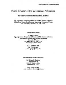
tions where each configuration is denoted by coni fig(RMRNn, i), 0 £ i £ n. Let r = 2 , then config(RMRNn, i) i consists of r = 2 rings R0, R1, º, Rr−1 stacked in a pipelined n-i fashion such that each ring has k = 2 processors. For 0 < j < r − 1 every processor in Rj is connected to a processor in Rj+1 and Rj−1. The input of each processor in R0 is multiplexed between an external input channel and the output of a processor in Rr−1. Analogously, the output of each processor in Rr−1 is demultiplexed between an external output channel and the input of a processor in R0. Given that the RMRNn is in configuration config(RMRNn, i), a processor p is in ring Rj iff p mod r = j. Also, processor p is connected to processors ((p + r) mod N) and ((p − r) mod N) in ring Rj via bidirectional links. Furthermore, we say that processor p is in position q in the ring Rj iff p div r = q. If 0 < j < r − 1 then there are bidirectional links between processors p and p + 1 and between processors p and p − 1. If j = r − 1 then there is a demultiplexed link between processor p and an external output channel. Conversely, processor p is connected to an external input channel via a multiplexed link if j = 0. For example, Figs. 1a and 1b show an RMRN4 system of 16 processors in configurations config(RMRN4, 1) and config(RMRN4, 2), respectively. In config(RMRN4, 1) we have two rings R0 and R1 where R0 consists of processors {0, 2, 4, 6, 8, 12, 14} and R1 consists of processors {1, 3, 5, 7, 9, 11, 13, 15} (Fig. 1a). In config(RMRN4, 2) we have four rings R0, R1, R2, and R3 where R0 consists of processors {0, 4, 8, 12}, R1 consists of processors {1, 5, 9, 13}, R2 consists of processors {2, 6, 10, 14}, and R3 consists of processors {3, 7, 11, 15} (Fig. 1b).

Fig. 1. RMRN4 in configurations 1 and 2.

2.2 Connections to the External Input/Output Channels The input and output control switches that provide connections to the external input and output channels respectively are straightforward to design. These switches are designed to check whether the last i bits of the processor address p are all 0 or 1, respectively. In config(RMRNn, i) i with r = 2 , there is a link between the external input chani nel and processor p iff p mod r = p mod 2 = 0 (i.e., p is in R0)

Authorized licensed use limited to: University of Georgia. Downloaded on November 11, 2008 at 11:29 from IEEE Xplore. Restrictions apply.

294

IEEE TRANSACTIONS ON PARALLEL AND DISTRIBUTED SYSTEMS, VOL. 8, NO. 3, MARCH 1997

and the input control signal IN is high else p is connected to the output of processor (p − 1) mod N. Conversely, iff p i mod r = p mod 2 = r − 1 and the output control signal OUT is high, then processor p is connected to the external output channel, else processor p is connected to the input of proci essor (p + 1) mod N. Calculating mod 2 is equivalent to examining the last i bits of the n bit address of processor p, i i i.e., p mod 2 = 0 or p mod 2 = r − 1 iff the last i bits of p are all 0 or all 1, respectively. Thus, the input control switch needs to check whether or not the least significant i bits of the processor address are all 0 whereas the output control switch needs to check whether or not the least significant i bits of the processor address are all 1. The hardware for the input/output switches is described in Section 5.1.

2.3 The Reconfiguration Switching Network A multistage switching network enables the RMRN to reconfigure itself from config(RMRNn, i) to config(RMRNn, j) where 0 £ i, j £ n and i π j. In config(RMRNn, i), processor p is i i connected to processors (p + 2 ) mod N and (p − 2 ) mod N. The function that the switching network needs to perform is related to that of a perfect shuffle network [37] and the barrel shifting network [25], but it is not exactly identical to either of them. The switching network is built up in the same way a shuffle network is, and, in fact, does contain some shuffle and unshuffle constituents. However, since it does not perform at all like a shuffle, it is unrelated functionally to the shuffle network. The relation to the barrel shifter is functional. The switching network serves to configure connections in a manner similar to how a barrel shifter would configure the bits of an operand. However, it is not constructed at all like a barrel shifter, so it is unrelated structurally to the barrel shifter. Section 5.2 details the hardware implementation of the reconfiguration switching network. The switching network bears structural and functional resemblance to the other hypercubic multistage interconnection networks such as the butterfly network [4], omega network [15], [19], [21], [30], delta network [28], baseline network [39], and the banyan network [14]. It can be shown in a straightforward manner that the interconnection links in a single stage of the butterfly network are contained within a specific configuration of the RMRN topology. This property can be proved in a manner analogous to the proof of Property 4 presented in the following subsection. Leighton [22] has shown the other commonly encountered multistage interconnection networks, i.e., omega, baseline, delta, and banyan, to be variants of the butterfly network. In [22], Leighton has presented a class of graph similarity transformations for systematically transforming the other networks into an equivalent representation in terms of the butterfly network. This implies that the various stages of the omega, baseline, delta, and banyan networks can also be shown to be contained within specific configurations of the RMRN topology. Since the reconfiguration switching network for the RMRN is a hierarchical multistage network like the butterfly network, the number of elementary switching elements needed to implement a reconfiguration switching network for N processors scales as O(N log2 N). Although the as-

ymptotic hardware complexity of O(N log2 N) is not attractive for very large values of N, it is manageable for moderate values of N. The O(N log2 N) hardware complexity is offset by the fact that the switching network is modular and hierarchically expandable and the expansion can be done using a single logical component as a building block. For example, one could use the switching network for RMRN4 as a building block for larger systems. One of the most important properties of the switching network is that each processor in RMRNn needs four bidirectional channels irren spective of the value of N = 2 . Since the connectivity of each node in RMRNn is fixed, the number of interprocessor communication links grows linearly with the system size n N = 2 . The RMRN thus satisfies an important criterion for a general purpose reconfigurable multiprocessor. In the following sections we explore some other important properties of the RMRN which underscore its viability for computer vision problems.

2.4 Basic Properties of the RMRN Topology We state and prove some important properties of the RMRN topology. i

j

PROPERTY 1. All 2D mesh topologies of size 2 ¥ 2 are subsets of the RMRNn where i + j = n. i

j

i

j

PROOF. Consider a grid with 2 rows and 2 columns such that i + j = n. Consider a position (k, l) in the grid. Under a row-major mapping, the processor address at position (k, l) is given by j

p = 2 k + l, 0 £ k £ 2 − 1, 0 £ l £ 2 − 1 The processor p is connected to its four nearest neighbors at locations (k − 1, l), (k + 1, l), (k, l − 1), and (k, l + 1) with the corresponding processors at these locations denoted by pn, ps, pe, and pw, respectively. Under the row-major mapping the processor addresses pn, ps, pe, and pw are given by:

b g = 2 b k + 1g + l = p + 2

j j pn = 2 k - 1 + l = p - 2

ps

j

j

pe = 2 j k + l + 1 = p + 1 pw = 2 j k + l - 1 = p - 1 j

Consider the RMRNn in config(RMRNn, j) with 2 rings n-j i each ring containing 2 = 2 processors. Under the row-major mapping, the processor p at grid location (k, l) is mapped onto the kth position in the lth ring. From the structural property of the RMRNn in config(RMRNn, j) processor p is connected to processors p j j + 2 and p − 2 in the lth ring and processors p + 1 and p − 1 in the (l + 1)th and (l − 1)th ring, respectively. Thus, it is clear that the the RMRNn in config(RMRNn, j) i j embeds the connectivity pattern of a 2 ¥ 2 mesh. This proves the property that all 2D mesh topologies of i j size 2 ¥ 2 are subsets of the RMRNn where i + j = n. † n

PROPERTY 2. The n-cube (i.e., a hypercube with N = 2 processors) can embed all possible configurations of the RMRNn (though not simultaneously). PROOF. See Appendix A.

Authorized licensed use limited to: University of Georgia. Downloaded on November 11, 2008 at 11:29 from IEEE Xplore. Restrictions apply.

BHANDARKAR AND ARABNIA: PARALLEL COMPUTER VISION ON A RECONFIGURABLE MULTIPROCESSOR NETWORK

PROPERTY 3. The configuration config(RMRNm, j) is a subconfiguration of config(RMRNn, i) whenever m < n, j < i, and n − m = i − j. Thus config(RMRNm, j) is a subset of config(RMRNn, i) with the connectivity pattern preserved. PROOF. The processor address p in config(RMRNn, i) can thus be decomposed as p = pmpn−m where the lowerorder n − m bits specify a particular subconfiguration of the type config(RMRNm, j) and the higher-order m bits specify the address p¢ within the subconfiguration config(RMRNm, j). Consider a processor p in config(RMRNn, i). From the definition of config(RMRNn, i), i p is adjacent to processors pr = (p + 2 ) mod N and pl = i (p − 2 ) mod N. In the configuration config(RMRNm, j), n-m the address of p is given by p¢ = p div 2 . The address of pr in config(RMRNm, j) is given by pr¢ = pr div 2 n

-m

= p div 2n m

e

n-m

Since p div 2

i n = p + 2 div 2

e j j + e2 div 2 j. n- m

i

i

-m

n-m

= p¢ and 2 div 2

i

i-j

= 2 div 2

j

= 2 , we

get the result pr¢ = p¢ + 2 j . Similarly, it can be shown that pl¢ = p¢ - 2 j . Thus config(RMRNm, j) is a subset of config(RMRNn, i) with the connectivity pattern preserved. † PROPERTY 4. Any algorithm which uses the communication links along a single dimension of the n-cube at any given point in time can be mapped to the RMRNn. PROOF. Let p(i) represent the processor whose n bit address differs from that of processor p only in the ith bit. Let p[i] denote the ith bit in the processor address p. Let Fin be the collection of edges in the n-cube in the ith dimension, i.e., Fin = {( p , p(i ))}. Then F0n , K , Fnn- 1 is a one-factor of the n-cube. It can be easily proved that Fin à config( RMRN n , i ). Without loss of generality, we may assume that p[i] = 0 and p(i)[i] = 1. Therefore p(i) i = p + 2 which means that p and p(i) are connected in config(RMRNn, i). Let A(p) denote the A register in processor p. Let the statement config(n, i) reconfigure RMRNn in config(RMRNn, i). Also, let left(p), right(p), i

next(p), and previous(p) denote the processors (p − 2 ) i

mod N, (p + 2 ) mod N, (p + 1) mod N, and (p − 1) mod N, respectively, in config(RMRNn, i). The statements A(p) Æ A(p(i)) and A(p) ¨ A(p(i)) in an algorithm for the ncube which move the contents of the A register of p to the A register of p(i) and vice versa along the ith dimension edge (p, p(i)) are, respectively, equivalent to the following statements on the RMRNn: config(n,i); IF (p[i] = 0) THEN A(p) –> A(right(p)) ELSE A(p) –> A(left(p));

This completes the proof of Property 4.

295

†

In summary, Property 1 states that the RMRNn can be configured into a variety of mesh topologies. In fact, we have proved that the RMRNn in config(n, i) contains as its i n-i subset a 2 ¥ 2 processor 2D wrap-around (i.e., toroidal) mesh. Property 2 shows how the n-cube can be used to simulate the behavior and function of the RMRNn. In fact, any given configuration of the RMRNn is a subset of the ncube. Property 3 shows that the RMRNn possesses an elegant recursive property with regard to its structure in a manner similar to the n-cube. In general, config(RMRNn, i) n-m subconfigurations of the type conwould contain 2 fig(RMRNm, j) such that m < n, j < i, and n − m = i − j. The condition n − m = i − j ensures that the number of processors in each ring of config(RMRNn, i) and config(RMRNm, j) is the same. If the RMRN is represented as a graph with the processors as nodes and the interprocessor links as arcs between nodes, then each of the subconfigurations config(RMRNm, j) would constitute a subgraph of the config(RMRNn, i). This property is important because it enables recursive decomposition of a procedure into independent subprocedures which could then be executed concurrently on individual subconfigurations. The usefulness of this property will be brought out in Sections 3 and 4 wherein we describe certain imaging operations that are to be performed in parallel on subimages or windows within the entire image. A subimage or window will be shown to essentially define a subconfiguration within the RMRN. Property 4 shows that the edges along a given dimension of the n-cube are contained within a specific configuration of the RMRNn. This result is of special significance since it allows a wide class of algorithms designed for the ncube to be mapped onto the RMRNn without loss of performance, assuming that the overhead in reconfiguration is not excessive. Any algorithm which uses the communication links along a single dimension of the n-cube at any given point in time can be mapped to the RMRNn in O(1) time. In summary, the RMRNn in any single configuration is a proper subset of the n-cube, whereas the edges along a specific dimension of the n-cube are a proper subset of the RMRNn. This implies that the RMRNn in any given configuration is more restrictive and hence less powerful than the n-cube. However, it should be noted that a vast majority of algorithms that use the n-cube in the SIMD or SPMD (and sometimes even in the MIMD) modes of parallelism, use the edges of the n-cube along one specific dimension at a given time. One can therefore conclude that the RMRN topology, on account of its reconfigurability, provides the same generality in practice as the n-cube for a large class of problems. In fact, the RMRN can be seen to offer a costeffective alternative to the n-cube architecture without substantial loss in performance.

and

3 SOME BASIC OPERATIONS AND ALGORITHMS ON THE RMRN

config(n,i); IF (p[i] = 0) THEN A(p) X(left(p)); ENDFOR END; Fig. 8. Data circulation using reconfiguration.

Alternatively, the data circulation operation can be accomplished using a single configuration of the RMRNn, i.e., n config(RMRNn, 0) which consists of a single ring of N = 2 processors. The O(N) algorithm for the data circulate operation which uses a single configuration of the RMRNn is outlined in Fig. 9. The advantage of this algorithm over the one in Fig. 8 is that the latter entails O(N) calls to config(◊, ◊) whereas the former involves a single call to config(◊, ◊). Since reconfiguration in a practical system involves some overhead, the algorithm in Fig. 9 could be expected to run faster than the one in Fig. 8 although both algorithms have an asymptotic complexity of O(N).

299

within the RMRN. The rotate operation is then carried out in parallel in each window (i.e., by the processors in each subconfiguration). If we are interested in config(w, k) in a w window of size W = 2 , then RMRNn has to be placed in config(n, n − w + k). This ensures that config(w, k) is a proper subconfiguration of config(n, n − w + k) (Property 3). In n w RMRNn with N = 2 , processors a window of size W = 2 is defined by appropriately assigning values to (n − w) bits in the address of the processors. The address of the processor within the window is given by appropriately masking the lower order (n − w) bits in the address of the processor (Property 3). Let p{w} denote the address of the processor w after the masking operation for a window of size W = 2 has been carried out for RMRNn. We can see that p{w}, right(p{w}), and left(p{w}) in config(w, k) refer to processors p, right(p), and left(p) respectively in config(n, n − w + k) since the connectivity pattern is preserved in subconfigurations of the RMRNn (Property 3). n In RMRN2n with N2 = 22 processors a window of size w

W ¥ W = 22 is defined by appropriately assigning values to 2(n − w) bits in the address of the processors. The address of the processor within the window is given by appropriately masking the lower order 2(n − w) bits in the address of the processor. The address of the processor after the masking w

operation for a window of size W ¥ W = 22 has been carried out is denoted by p{2w}. The kth bit in the masked address is then denoted as p{2w}[k]. The rotate operation within a window could be described thus: k A 1D rotate operation by 2 pixels in a window of size 2 2w W = 2 can be described as: k

2

for rotate left: R(p) ¨ R((p + 2 ) mod W ) k 2 for rotate right: R(p) ¨ R((p − 2 ) mod W ) k

A 2D rotate operation by 2 pixels can be described as: k

Circulate(X, n) BEGIN config(n, 0); FOR i:= 0 to (2**n) - 1 DO X(p) –> X(right(p)); END; Fig. 9. Data circulation using a single configuration.

for rotate right: R(i, j) ¨ R(i, (j − 2 ) mod W) k for rotate left: R(i, j) ¨ R(i, (j + 2 ) mod W) k for rotate up: R(i, j) ¨ R((i + 2 ) mod W, j) k for rotate down: R(i, j) ¨ R((i − 2 ) mod W, j) A generic rotate operation within a window is described w in Fig. 10. For a 1D rotation in a window of size W2 = 22 the RotateWin procedure would have to be invoked thus: k

Rotate left by 2 pixels: RotateWin(R, 2n, k, 2w-1,

3.2 Some Basic Imaging Operations on the RMRN Given a 2D image G = {G(i, j); i, j Œ [0, N − 1]} and an RMRN n with N2 = 22 processors where the value of the pixel (i, j) is stored in register R(p) of processor p = iN + j (i.e., row-major mapping). We will occasionally refer to the processor p = i N + j by the ordered pair (i, j) keeping in mind that the rowmajor mapping is a bijection since i = p div N and j = p mod N. Similarly, we will also occasionally refer to the register R(p) as R(i, j).

3.2.1 Rotate Operation Within a Window One of the basic imaging operations that could be performed on the RMRN is the rotate or the cyclic shift operation performed in a subimage or window within the entire image. The window essentially defines a subconfiguration

2w, 0)

k

Rotate right by 2 pixels: RotateWin(R, 2n, k, 2w-1, 2w, 1) w

For a 2D rotation in a window of size W2 = 22 the RotateWin procedure would have to be invoked thus: k

Rotate down by 2 pixels: RotateWin(R, 2n, w+k, 2w-1, 2w, 1) k

Rotate up by 2 pixels: RotateWin(R, 2n, w+k, 2w-1, 2w, 0) k

Rotate left by 2 pixels: RotateWin(R, 2n, k, w-1, 2w, 0)

k

Rotate right by 2 pixels: RotateWin(R, 2n, k, w-1, 2w, 1)

Authorized licensed use limited to: University of Georgia. Downloaded on November 11, 2008 at 11:29 from IEEE Xplore. Restrictions apply.

300

IEEE TRANSACTIONS ON PARALLEL AND DISTRIBUTED SYSTEMS, VOL. 8, NO. 3, MARCH 1997

RotateWin(R, n, s, r, w, flag) BEGIN config(n, n-w+s); IF (p{w}[s] = 0) THEN R(p) –> R(right(p)) ELSE R(p) –> R(left(p)); FOR b:= s+1 to r DO BEGINFOR config(n, n-w+b); IF (flag = 0) THEN IF (p{w}[b-1] = 1) AND... AND (p{w}[s] = 1) THEN IF (p{w}[b] = 0) THEN R(p) –> right(R(p)) ELSE R(p) –> left(R(p)); ENDIF; ELSE IF (p{w}[b-1] = 0) AND... AND (p{w}[s] = 0) THEN IF (p{w}[b] = 0) THEN R(p) –> right(R(p)) ELSE R(p) –> left(R(p)); ENDIF; ENDIF; ENDFOR; END; Fig. 10. Rotate operation within a window. 2w

The rotate operation within a W ¥ W = 2 window contains O(w) = O(log2 W) unit hops. The broadcast, combine and circulate operations can be similarly performed within a predefined window. The broadcast and combine operations would contain O(w) = O(log2 W) unit hops and the circulate operation would contain O(W) unit hops for a window of w size W = 2 . The algorithms for the broadcast, combine and circulate operations within a window are similar to the ones already described and hence will not be repeated here.

3.2.2 Accumulate Operation Each processor j has an array A[0 º M − 1] of size M. A[i](j) refers to the element A[i] in processor j. In addition, each processor has a value in its I register. After the accumulate operation, the M elements of the array A in each processor j are such that: A[i](j) = I((j + i) mod N), 0 £ i < M, 0 £ j < W w

where W = 2 is the window size. The accumulate operation can be performed as a minor modification of the circulate operation within a window using the following lemma from Ranka and Sahni [33] LEMMA 3.1. Let I0, I1, º, IW−1 denote the initial values in I(0), I(1), º, I(W − 1). Let index(j, i) be such that index(j, i) is in A(j) following the ith iteration of the for loop in the data circulation algorithm shown in Fig. 8. Initially index(j, i) = j. For every i > 0, index(j, i) = index(j, i − 1) ≈ f(w,i) where ≈ denotes the EXOR operation and f(w, i) is as 2 defined in Section 3.1.3. The value of index(j, i) essentially conveys the address (within the window) of the originating processor during each iteration of the circulate operation. The algorithm for the accumulate operation is given in Fig. 11. The data accumulate operation Accumulate(A, I, M) can be performed

in O(M + log2 (N/M)) unit hops on the RMRNn. Accumulate(A, I, M) {Each processor accumulates in array A the I values of the next M processors. The window size is M = 2**m} BEGIN A[0] = I; index = p; FOR i:= 1 to 2**m - 1 DO BEGINFOR config(n, f(m,i) + n - m); IF (p{m}[f(m,i)] = 0) THEN I(p) –> I(left(p)) ELSE I(p) –> I(right(p)) index := index EXOR 2**f(m,i); location := (index - p{m}) mod M; A[location] := I; ENDFOR; END; Fig. 11. Accumulate operation within a window.

4 LOW- AND INTERMEDIATE-LEVEL VISION OPERATIONS ON THE RMRN The primitive operations defined in the previous section can be extended to design operations for low- and intermediate-level vision on the RMRN. Typical examples of lowlevel vision operations are image transforms such as the Fast Fourier Transform (FFT), and convolution for edge detection, image filtering, image smoothing, and feature detection via template matching. A typical example of intermediate-level vision is feature extraction via the Hough Transform. We consider the implementation of these operations on the RMRN.

4.1 The Fast Fourier Transform For the purpose of discussion, we have selected one of the most widely known decimation-in-frequency FFT algorithms described in [16]. First, we describe how the onedimensional FFT algorithm can exploit the RMRN system and then address the problem of expanding the algorithm to handle the two-dimensional case. Let s(m), m= 0, 1, º, M − 1 be M samples of a time function. The Discrete Fourier Transform of s(m) is defined to be the discrete function X(j), j = 0, 1, º, M − 1 given by: M -1

b g  samf ◊ W

X j =

jm

m=0

i M where W = e 2p , i = -1 , and j = 0, 1, º, M − 1. n In the RMRNn where N = 2 = M/2, processor p initially contains s(p) and s(p + M/2), where 0 £ p < N. The FFT algorithm consists of log2 M stages of computation and log2 (M/2) = log2 N stages of parallel data transfers (unit hops). A process known as the butterfly (Fig. 12a) is executed M/2 times (in parallel) at each stage of computation. For example, for a 16-point FFT, eight butterfly processes are performed in parallel at each stage of computation where each process receives two inputs and produces two results. Each processor, however, outputs only one of the two results to another processor, keeping the other in its memory. At the

Authorized licensed use limited to: University of Georgia. Downloaded on November 11, 2008 at 11:29 from IEEE Xplore. Restrictions apply.

BHANDARKAR AND ARABNIA: PARALLEL COMPUTER VISION ON A RECONFIGURABLE MULTIPROCESSOR NETWORK

ith parallel data transfer stage a processor p outputs its X value if p[i] = 1 else it outputs its Y value. It is only at the very last stage of computation that each processor outputs both results of its butterfly process (to the outside world). The actual interconnection network (i.e., butterfly network) required to perform the four stages of the 16-point FFT is shown in Fig. 12b where the data is considered to flow from left to right.

301

FFT(M, n) {There are N=2**n processors and N=M/2} BEGIN config(n, n); A(p) := s(p); B(p) := s(p + M/2); k := p; X(p) := A(p) + B(p); Y(p) := (A(p) - B(p)) * W**k; {** denotes exponentiation} FOR i = n-1 DOWNTO 0 DO BEGINFOR config(n, i); IF (p[i] = 1) THEN X(p) –> A(left(p)); B := Y; ELSE Y(p) –> B(right(p)) A := X; ENDIF; k := (2*k) mod N; X(p) := A(p) + B(p); Y(p) := (A(p) - B(p)) * W**k; ENDFOR; END; Fig. 13. M-point FFT on the M/2 processor RMRN.

Fig. 12. (a) Butterfly process (b) Interconnection pattern for the 16point FFT on the RMRN3.

The FFT algorithm described in Fig. 13, performs the Mpoint FFT calculations using log2 (M/2) = log2 N parallel n data transfers (unit hops) on the RMRNn with N = 2 processors. This is a lower bound on the number of parallel data transfers required to perform an M-point FFT when the M points are initially distributed over M/2 processors [16]. The number of parallel butterfly operations performed is log2 M, where each butterfly involves two complex additions and one complex multiplication in each processor. The asymptotic complexity of the algorithm is O(log2 (M/2)) = O(log2 N). The 2D FFT of an N ¥ N image can be computed by first computing the 1D FFT of each row of the image followed by the 1D FFT of each column of the resulting image.

4.2 Convolution for Edge and Feature Detection The convolution operation is a fundamental operation used in both edge and feature detection. In both cases, the underlying image is convolved with a template or a set of templates and the edges or features of interest are deemed to be points in the image where the output of the convolution has a maximum. A one-dimensional convolution is given by the relation: M -1

Ci =

 I bi + k g mod N

◊T k

0£i£N

(4)

k =0

where I[0 º N − 1] is the 1D image and T[0 º M − 1] is the template. The convolved output is C[0 º N − 1]. A twodimensional convolution is given by the relation: M -1 M -1

C i, j =

  I bi + k g mod N , b j + lg mod N

◊ T k, l

(5)

k =0 l=0

where 0 £ i, j £ N, I[0 º N − 1, 0 º N − 1] is the N ¥ N im-

age, T[0 º M − 1, 0 º M − 1] the M ¥ M template and C[0 º N − 1, 0 º N − 1] the N ¥ N image resulting from the convolution. The two-dimensional convolution can be decomposed into a series of 1D convolutions and summations [31], [32]: M -1

C¢ i , j , k =

 I bi + k g mod N , b j + lg mod N

◊ T k, l

l=0 M -1

C i, j =

 C¢ i , j , k

(6)

k =0

For the 1D convolution operation we assume that there are N processors in the RMRN and the vector I is mapped onto the RMRN using the identity mapping, i.e., I(i) is mapped onto processor i. We also assume that there are (N/M) copies of the template T on the RMRN with one copy in each subconfiguration of M processors. Within each subconfiguration, the mapping of T is identical to the mapping of I. Since each processor has O(M) memory, the most effective strategy is to perform a data accumulate operation on the I values such that each processor has all the I values necessary to compute a single value of the output vector C. The mapping of the output vector C on the RMRN is identical to the mapping of the input vector I. Let f(n, i) denote the ith number in the palindromic exchange sequence in (3). The code for 1D convolution with O(M) memory per processor is given in Fig. 14. The template is stored in the T register and the final result in the C register of each processor. For the 2D convolution operation we assume that an n RMRN2n with N2 = 22 processors is available. We assume an identity mapping for the image I, i.e., I(i, j) is contained in the I register of the (i, j)th processor. We also assume that there are (N/M)2 copies of the template T; one copy in each subconfiguration of M2 processors. Within each subconfiguration the mapping of T(I, j) is identical to the mapping

Authorized licensed use limited to: University of Georgia. Downloaded on November 11, 2008 at 11:29 from IEEE Xplore. Restrictions apply.

302

IEEE TRANSACTIONS ON PARALLEL AND DISTRIBUTED SYSTEMS, VOL. 8, NO. 3, MARCH 1997

of I(i, j). The mapping of the output image C(i, j) is also identical to that of I(i, j). The code for the 2D convolution can be derived by decomposing it into a series of 1D convolutions and summations using (6). Both the 1D and 2D convolutions can be performed on the RMRN in with the same asymptotic order of complexity as would result by implementing them on the hypercube [31], [32], [20], [12] in an SIMD or SPMD mode parallelism. The 1D convolution can be performed in O(M + log2 M + log2 N) unit hops whereas the 2D convolution can be performed in O(M2 + log2 M + log2 N) unit hops. procedure Convolve1D(M) BEGIN ACCUM(A, I, M); C := 0; index := p mod M; FOR j:= 1 to M DO BEGINFOR C := C + A[index] * T; m := log2(M); {log2() is log to the base 2} l := f(m, j); config(n,l); IF (p[l] = 0) THEN T(p)