PARALLEL COMPUTING ADAPTIVE SIMULATED ANNEALING SCHEME FOR FUEL ASSEMBLY LOADING PATTERN OPTIMIZATION IN PWR’s Hyun Chul Lee, Hyung Jin Shim, and Chang Hyo Kim Nuclear Engineering Department Seoul National University Seoul, Korea
[email protected] ;
[email protected] ;
[email protected]
ABSTRACT An adaptive control scheme of simulated annealing(SA) parameters derived from polynomial-time cooling schedule is presented in terms of the efficiency enhancement of the SA algorithm. The paralle l computing adaptive SA optimization scheme which incorporates the optimization-layer-by-layer(OLL) neutronics evaluation model is then applied to determining the optimum fuel assembly(FA) loading pattern(LP) in Korea Nuclear Unit 11(KNU 11) PWR using seven Pentium personal computers(three Pentium II 266 MHz and four Pentium Pro 200 MHz). It is shown that the parallel scheme enhances the efficiency of the SA optimization computation significantly but that it can get trapped in local optimum LP more frequently than the single processor SA scheme unless one takes preventive steps. As a way to prevent trapping of the parallel scheme in local optimum, we proposed using multiple seed LP's instead of a single LP with which the individual processors start each sta ge and discussed how to determine the multiple seed LP's. Because of high efficiency of the parallel scheme, acceptability of hybrid neutronics evaluation model which is slower but more accurate than OLL model into parallel optimization calculation is examined from the standpoint of the computing time. By demonstrating that the FA LP optimization calculation for the equilibrium cycle core of the KNU 11 PWR can be completed in less than an hour on seven Pentiums, we justified the routine utilization of the hybrid model in the parallel SA optimization scheme.
1. INTRODUCTION The simulated annealing(SA) algorithm has presented a powerful tool for the in-core fuel management optimization computations.1,2 But it has a disadvantage of lengthy turnaround time by requiring neutronics evaluation of several tens of thousands of trial loading patterns(LP's) in the optimization process. As a way to overcome this, Parks et al. 3 examined earlier the parallel computing SA capability with the parallel implementation of FORMOSA on an IBM 3090 vector machine with four processors. Recently we presented personal computer(PC)-based parallel computing SA fuel assembly(FA) LP optimization schemes4 which incorporate a fast-running optimization-layer-by-layer(OLL) neural networks neutronics evaluation model (OLL model hereafter). 5 We demonstrated that they are very effective in reducing the turnaround time of the FA LP optimization computations in PWR but that they have a drawback to get trapped in the local optimum LP more frequently than the single processor SA scheme. The objectives of this paper is to reinvestigate the effectiveness of parallel computing SA optimization schemes by introducing the adaptive control of the SA parameters, to present a way to reduce the probability of any given parallel optimization run getting trapped in the local optimum LP, and to examine acceptability of incorporating more accurate but more time-consuming neutronics evaluation model than the OLL model from the standpoint of computing time. 1
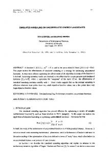
The self-adaptive control of annealing parameters is prerequisite to minimize the total number of LP sampling and thus reduce the computing time of the SA optimization calculations. The FORMOSA code is known to use the self-adaptive control scheme proposed by Huang et al..6,7 Except for reference 6 where the adaptive SA scheme of the FORMOSA code was first discussed, the details on it are rarely available in open literature. Here we introduce a slightly different adaptive scheme derived from polynomial-time cooling schedule 8 , in setting the initial temperature, the temperature decrement ratio, and the stopping criteria of the optimization calculation and discuss its application to, and its effectiveness in, the FA LP optimization calculations. In order to take advantage of the efficiency of the parallel scheme, one has to reduce the probability that it gets trapped in the local optimum LP. 4 We will discuss the cause for this. Through numerical experiments we will show that the probability for trapping in the local optimum LP depends on the way how one decides the seed LP’s with which individual processors start at the beginning of each stage. Then we will suggest using multiple seed LP’s to avoid trapping in the local optimum and present how to determine them. The OLL model is an extremely fast neutronics evaluation tool. To use it, one has to spend the extra computing time for training all the necessary OLL networks for neutronics evaluation and sacrifice a certain degree of computational accuracy as well. In addition, the trained OLL model has a limited utility because they can be applicable only to the specific cycle core that has provided the training set of neutronics data. In order to overcome these disadvantages of the OLL model, we devised a hybrid neutronics model which employs the nodal method for global core calculation and utilizes the OLL networks only for prediction of the pin power peaking factors(PPPF's) of the individual FA's. The hybrid model is more accurate than, and free from the above-mentioned disadvantages of, the OLL model. Even though it is more time-consuming than the OLL model, we will demonstrate that the FA LP optimization can be carried out in less than an hour using the seven Pentium PC’s(three Pentium II 266 MHz and four Pentium Pro 200 MHz) available at our graduate research laboratory and therefore the routine utilization of the hybrid model is justified.
2. STATEMENT OF THE OPTIMIZATION PROBLEM The FA LP optimization problem here is to determine the fuel loading matrix X that will maximize the end-of-cycle(EOC) critical soluble boron concentration, sb(X), under the radial pin power(F∆H ) and maximum FA discharge burnup(Bmax) constraints using the augmented cost function2 , f(X),
f ( X ) = −sb ( X ) + θ1
L
NA
[(
)]
∑∑ max Pml ( X ) − F∆H ,0 + θ2 l =0 m =1
2
∑ max [( B NA
m =1
m
( X ) − Bmax ),0 ]
2
(1)
3. PARALLEL COMPUTING SA OPTIMIZATION SCHEME The SA optimization algorithm consists of generation of a new LP(Xnew) from the current LP(Xcur), evaluation and decision making on the acceptance of the Xnew according to the acceptance probability,
e − ∆f / c , if ∆f = f ( X new ) − f ( X cur ) > 0 P = , otherwise 1
(2)
In parallel computing SA scheme, N(>1) processors are employed simultaneously to follow the SA 2
optimization algorithm. As in the case of the single processor SA scheme, the whole process is divided into annealing stages in each of which the preset number of LP's are subject to SA sampling with the constant temperature parameter c set by the specified annealing schedule. A given stage usually ends either when the total number of the LP generation reaches the preset limit per stage(Nstg ) or when the number of the accepted LP's reaches the preset limit(Nacp). In reference 4, we presented three different parallel schemes. But here we consider only one parallel scheme designated as the scheme(II). In this scheme, all the N processors engage simultaneously in SA optimization process and one master processor communicates with all the other N-1 slave processors to count the total number of LP's that all the N processors have sampled and accepted. Thus all the processors complete a given stage at the same time by the stage end criteria(Nstg or Nacp) recorded on the master processor and start the next stage with the Xcur provided by the master processor.
4. SELF-ADAPTIVE CONTROL OF THE SA PARAMETERS The SA optimization algorithm requires setting the initial temperature, c0 , temperature decrement ratio, αk, and the stopping criteria. For the self-adaptive control of these parameters, we use a polynomial-time cooling schedule presented in reference 8. In this schedule, the initial temperature is determined by (+)
∆f c0 = m2 ln m2 χ − m1 (1 − χ)
(3)
where the χ is the initial acceptance ratio, and m1 and m2 are the number of cost increasing and cost (+ ) decreasing LP's, respectively. The ∆f is the average of the cost difference over the m2 cost increasing LP changes. The temperature decrement ratio αk is given by
αk =
1 , ck ln( 1 + δ ) 1+ 3σk
(4)
where the ck and σk are the temperature and the standard deviation of the cost function at the stage k, respectively. The distance parameter, δ, is some small positive constant close to zero, and is a measure of closeness of equilibrium distributions of two Markov chains at two successive cooling stage. To end the optimization computation, we use the stopping criteria derived as follows :
f f
− f opt − f opt ∞ k
≈
∂ f 1 ⋅ c k f ∞ − f opt ∂c
≈
c c = ck
(
where
f
∞
= the mean cost function at initial hot temperature,
3
(σ k )2 f
∞
)
− f kbest ck
< εs ,
(5)
f
k opt
= the mean cost function at stage k,
f = the cost function of the optimum LP, f kbest = the cost function of the best LP recorded till the stage k, ε s = the stopping parameter. Equation (5) states that the distance between the between the ∂ f σ = 2 ∂c c
2
f
∞
and f opt is a small fraction of the distance and f opt . In driving Eq. (5), we assumed that f varies linearly with c and used f
k
along with an approximation, f opt ≈ fkbest .
The initial temperature and stopping criteria are different from those presented by Huang et al. 7 But the temperature decrement ratio of Eq.(4) can be shown to be similar to the one presented by Huang et al. and adopted by FORMOSA code. In this conjunction, let us note λck/σk 0 P = e 1 , otherwise
(i = 1,2,L N − 1)
(8)
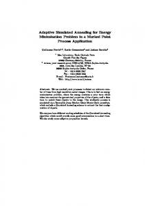
The LP which is last accepted becomes the seed LP of the processor. The parameter p(>1) in Eq. (8) is chosen to create hotter condition, so that a given processor can accept the current LP of other processors with high probability. By determining the seed LP's of N processors at the beginning of each stage this way, one can avoid starting the stages with only a single seed LP and thus hopefully reduce the tendency of the parallel scheme getting trapped in the local optimum. Fig ure 5 depicts the stagewise standard deviation of the parallel scheme with the multiple seed LP's at each stage.. The stagewise standard deviation of the parallel scheme now varies in a very similar way as that of the single processor SA scheme. The higher the p is, the slower the change in the standard variation becomes and thus the number of the total LP sampling increases. Table III shows performance of the parallel adaptive SA scheme with multiple seed LP’ s. We observed the p=3 is reasonable choice from the efficiency standpoint.
6.3 PARALLEL SA OPTIMIZATION WITH HYBRID NEUTRONICS MODEL The hybrid model is designed to overcome major disadvantages of the OLL model at the expense of the computing time. Table IV shows a comparison of the PPPF prediction accuracy of the hybrid and OLL models. The hybrid model can predict the PPPF with the mean and maximum relative errors less than 1 and 5 % with respect to 4 N/FA nodal calculation, respectively. In comparison, the OLL model shows much larger mean and maximum errors. Needless to mention, the higher PPPF prediction accuracy of the hybrid model is ascribed to the fact that the OLL networks in the hybrid model utilizes more informations than those in the OLL model. As for the computing time, the hybrid model takes about one second on Pentium II 266 MHz for a cycle burnup analysis of a given LP of the KNU 11 PWR on 10 burnup steps, while the OLL model takes only 50 milliseconds. Table V shows the performance of parallel SA optimization computations with the incorporation of the hybrid model on seven Pentiums. For a reasonable statistics, the 30 parallel optimization runs are made. The total number of LP sampling is about 15,000 on the average. The turnaround time of each optimization run is mostly less than an hour. The parallel scheme has produced near optimum LP's as frequently as the single processor scheme. The six to seven out of ten optimization runs has reached the near optimum LP. 6
CONCLUSIONS The adaptive control scheme of SA parameters introduced herein is slightly different from that of the FORMOSA code. The initial temperature setting, the stopping criteria, and use of the smoothed standard deviation in the temperature decrement ratio and the stopping criteria are new features that are straightforwardly implemented and contribute to efficiency enhancement of the SA optimization computations. The parallel SA scheme can overcome the major disadvantage of the lengthy turnaround time of the single processor SA optimization scheme. In order to avoid easy trapping of the parallel scheme in the local minimum LP, however, one must take the preventative scheme like use of the multiple seed LP's at each annealing stage that we suggested in this paper. The high efficiency of the parallel scheme may allow to incorporate the slower but more accurate neutronics model like the hybrid model than the OLL model into SA algorithm. We justified the incorporation of the hybrid model into the parallel SA scheme by demonstrating that the FA LP optimization of the KNU 11 PWR can be carried out in less than one hour with seven Pentiums. In conclusion, the parallel computing adaptive SA optimization scheme is very efficient and it can be carried out with little or no extra cost on computer facilities in the PC-affluent working environment of any fuel management groups nowadays. The acceptable turnaround time of less than an hour on seven Pentiums as well as the high success rate of getting near optimum LP per optimization run warrant the routine utilizatio n of the parallel computing adaptive SA optimization scheme on multiple personal computers.
ACKNOWLEDGEMENTS This work was supported partly by Korea Nuclear Fuel Company and partly by Korea Science and Engineering Foundation.
REFERENCES 1. D. J. Kropaczek and P. J. Turinsky, In-Core Fuel Management Optimization for Pressurized Water Reactors Using Simulated Annealing, Nucl. Tech., 95, 9 (1991). 2. J. G. Stevens, K. S. Smith, K. R. Rempe, and T. J. Downer, Optimization of Pressurized Water Reactor Shuffling by Simulated Annealing with Heuristics, Nucl. Sci. Eng., 121, 67 (1995). 3. G. T. Parks, P. J. Turinsky, and G. I. Maldonado, Scientific Excellence in Supercomputing, The IBM 1990 Contest Prize Papers, Vol. I, Balwin Press, Athens, GA (1992). 4.
J. H. Lee, H. C. Lee, and C. H. Kim, Parallel Computing Fuel Assembly Loading Pattern Optimization by Simulated Annealing Method, Trans. Am. Nucl. Soc. 80, 228 (1999).
5. J. H. Lee, H. J. Shim, C. S. Jang, and C. H. Kim, Incorporation of Neural Networks into Simulated Annealing Algorithm for Fuel Assembly Loading Pattern Optimization in a PWR, Proc. Int. Conf. on Phys. of Nuclear Science and Technology, Oct 5-8, 1998, Long Island, NY, USA, Vol. 1, p. 75. 6. D. J. Kropaczek, P. J. Turinsky, G. T. Parks, and G. I. Maldonado, The Efficiency and Fidelity of The In-Core Nuclear Fuel Management Code FORMOSA-P, Reactor Physics and Reactor Computations, Israel Nuclear Society and European Nuclear Society, Tel-Aviv (1994).
7
7. M. D. Huang, F. Romeo, and A. Sangiovanni-Vincentelli, An Efficient General Cooling Schedule for Simulated Annealing, IEEE Int. Conf. On Computer Aided Design, pp. 381-384 (1986) 8. E. Aarts and J. Korst, Simulated Annealing and Boltzmann Machines, John Wiley & Sons, New York, NY, USA (1989). 9. R. Diekmann, R. Lüling, and J. Simon, Problem Independent Distributed Simulated Annealing and Its Application, Technical Report PC², TR -003-93 (1993). 10. R. Otten and L. van Ginneken, The Annealing Algorithm, Kluwer Academic Publishers (1989). 11.
T. K. Kim and C. H. Kim, Verification of the Pressurized Water Reactor Analysis Codes : CASMO/NEMSNAP, Proc. Korean Nucl. Soc., Spring Meeting, Pohang, Korea, May 27-28 (1994).
12. P. S. Pacheo, Parallel Programming with MPI, Morgan Kautmann Publisher Inc., San Fransisco, USA (1997). (a) Hybrid Neutronics Evaluation Model. CASMO-3 Assembly Homogenization Two-Group CX’ s , ADFm power form function : F ( x,y )
NEMSNAP code for global core depletion analysis
NPm , Bm
NPm
m m m J gus , φgus , φgm J gus
Critical SB
m φgus
OLLnetworks for PPPF prediction
PPPFhom
PPPF = PPPFhom × peak value of F(x,y)
(b) OLL Networks-Based Neutronics Evaluation Model. CASMO-3 Assembly Homogenization
k ∞ , Σ a 2 m , κ Σf 2 m(m = 1, 2, …,NFA) power form function : F ( x,y ) ADFm
OLL-networks for global core depletion analysis
NPm , Bm , critical SB concentration NPm
OLLnetworks for PPPF prediction
PPPFhom
Figure 1. Hybrid and OLL Networks-Based Neutronics Evaluation Model.
8
PPPF = PPPFhom × peak value of F(x,y)
o0n = 1
1 w10 a
Σ
NP1 • • • NP 9 wh 0
φ2 xl / φ2
whm
φ2 yl / φ2
a
φ2 xr / φ2
a
s1n
f (s1n )
o1n
c
v0 v1 b
• • •
Σ
shn
( )
f s hn
o nh
c
• • •
φ2 yr / φ2 J 2 xl / φ2
Σ
J 2 yl / φ2 J 2 xr / φ2
wH 17
b
vh
vH s
n H
f (s Hn
)
Σ
b
PPPFhom
b
o nH c
a
J 2 yr / φ2 a
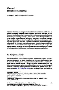
whm (m=0,1, … ,1 7, h = 0,1, …, H ) = weights for hidden neurons v h (h = 0, 1, … H , ) = weights for output neurons c f ( s ) = sigmoidal function defined by (1+e-s )-1 b
Figure 2. OLL Networks for Prediction of PPPFhom in Hybrid Neutronics Evaluation Model.
1000 Smoothing
Stdard Deviation of Cost Function
No Smoothing
100
10
1
0.1 0
20
40
60
80
Stage Index
Figure 3. Effect of Smoothing on Satgewise Standard Deviation of Cost Function
9
Standard Deviation of Cost Function
1000
S i n g l e P r o c e s s o r S A ( N acp = 5 0 , N stg = 5 0 0 ) Parallel SA with Single Seed LP(N acp = 5 0 , N stg = 5 0 0 ) 100
Parallel SA with Single Seed LP(N acp = 6 0 , N stg = 6 0 0 )
10
1 0
10
20
30
40
50
60
70
Stage Index
Figure 4. Stagewise Standard Deviation of Cost Function.
1000
Single Processor SA
Standard Deviation of Cost Function
P a r a l l e l S A w i t h M u l t i p l e S e e d L P (p =1.0) P a r a l l e l S A w i t h M u l t i p l e S e e d L P (p =3.0) P a r a l l e l S A w i t h M u l t i p l e S e e d L P (p =5.0)
100
10
1 0
10
20
30
40
50
60
70
Stage Index
Figure 5. Stagewise Standard Deviation of Cost Function.
10
80
Table I. Performance Comparison of Nonadaptive versus Adaptive SA Algorithms* ( N acp=50 , N stg=500 , χ=0.99 , λ=0.1 , εs=0.005 ) SA Algorithm
Nonadaptive SA
Adaptive SA (I)
Adaptive SA (II)
Adaptive SA ( III)
Initial Temperature c 0
Eq. (3)
Eq. (3)
Eq. (3)
Eq. (3)
σ
σ
σ
Adaptive SA (IV)
Adaptive SA (V)
Eq. (3)
Eq. (3)
Eq. (6) with
σk
Eq. (6) ) with
σ sk
Eq. (5) with
σk
Eq. (5) with
σ sk
Cooling Parameter α k
Constant (=0.95)
Stopping Criteria
Number of Accepted LP ’s < 2
Number of Accepted LP’s < 2
Mean Number of LP Sampling ± σ b Mean Number of Stages ± σ b
48059±4582
29480±1867
11213±11528
20963±10697
12343±2387
16975±1680
193±9
101±5
47±36
70±28
66±6
64±4
f opt ± σ
-434.2±10.3
-431.0±11.1
-380±50.4
-408.9±53
-418.4±16.4
-427.7±12.0
b
Eq. (6) with
s k
Eq. (6) with
(∆f )max k f
max k
−f
min k
s k
> 0.95
Eq. (6) with
(∆f )max k
a
f
max k
− f kmin
s k
> 0.98
a
*
Numerical results are derived from 30 independent optimization runs. Reference 7. b σ : standard deviation. a
Table II. Performance of Parallel Adaptive SA Scheme with Single Seed LP.* ( χ=0.99 , εs=0.005 ) Number of Stages
Total Number of LP Sampling
EOC Soluble Boron (ppm)
PPPF
Cost Function
Elapsed Time a (sec)
λ=0.1
46±6
10504±2907
401±31
1.461±0.012
-395.0±29.4
89±22
λ=0.07
67±11
15819±3948
409±23
1.460±0.011
-405.6±21.6
134±32
λ=0.05
92±20
20880±8043
417±27
1.462±0.010
-412.1±25.0
177±64
N acp=60 N stg=600
λ=0.1
48±4
13825±2605
410±20
1.458±0.012
-407.0±17.8
119±20
N acp=70 N stg=700
λ=0.1
52±4
18209±2859
413±26
1.458±0.008
408.9±24.0
148±18
N acp=80 N stg=800
λ=0.1
55±5
22572±3641
419±22
1.461±0.009
-414.2±20.2
185±30
Parameters
N acp=50 N stg=500
* a
Numerical results are derived from 20 independent optimization runs. On seven Pentium(Three Pentium II 266MHz and Four Pentium Pro 200MHz)
11
Table III. Performance of Parallel Adaptive SA Scheme with Multiple Seed LP.* ( Nacp =50 , N s t g=500 , χ =0.99 , λ=0.1 , εs=0.005 )
* a
Parameter p
Number of Stages
Total Number of LP Sampling
EOC Soluble Boron (ppm)
PPPF
Cost Function
Elapsed a Time (sec)
1.0
51± 4
12547± 1969
414± 23
1.455±0.008
-411.2± 22.2
113±18
3.0
67± 5
17951± 2170
430± 14
1.458±0.008
-427.8± 14.4
150±19
5.0
75± 4
20674± 1601
434± 12
1.461±0.008
-429.3± 12.9
174±16
7.0
82± 7
23696± 2680
436± 11
1.457±0.008
-433.5± 10.9
201±22
Numerical results are derived from 20 independent optimization runs. On seven Pentium(Three Pentium II 266MHz and Four Pentium Pro 200MHz)
Table IV. Comparison of the PPPF prediction accuracy of the hybrid and OLL models.
Hybrid Model Core Burnup State
a b
a
εave (%)
OLL Model b
ε max (%)
a
εave (%)
εmax (%)
4.77
1.60
11.26
3.48
1.20
8.70
2.90
0.97
4.80
BOC 0.91 ( 0 MWD/T ) MOC 0.74 (7000 MWD/T ) EOC 0.69 ( 14000 MWD/T ) εave = average relative error in PPPF prediction
b
ε max = maximum relative error in PPPF prediction.
*
Table V. Performance of Parallel Adaptive SA Algorithm with Hybrid Neutronics Evaluation Model ( N acp =50 , Ns t g=500 , χ=0.99 , λ =0.1 , εs =0.005 , p=3.0 ) Number of Stages
Number of LP's Sampled
CPU Time (min)
Elapsed a Time (min)
EOC Soluble boron (ppm)
PPPF
Mean value 65±3 15107± 1863 368±44 55± 6 432± 15 1.458±0.010 b ±σ * Numerical results are derived from 30 independent optimization runs. a On seven Pentium(Three Pentium II 266MHz and Four Pentium Pro 200MHz) b σ : Standard deviation.
12
Cost Function -430.7± 15.1