PARALLEL FAST LEGENDRE TRANSFORM 1. Introduction

PARALLEL FAST LEGENDRE TRANSFORM MA RCIA ALVES DE INDA Mathematics Department, Utrecht University Budapestlaan 6, Utrecht, 3584 CD, The Netherlands ROB H. BISSELING Mathematics Department, Utrecht University Budapestlaan 6, Utrecht, 3584 CD, The Netherlands and DAVID K. MASLEN Mathematics Department, Dartmouth College Hanover, NH 03755, U.S.A. ABSTRACT We discuss a parallel implementation of a fast algorithm for the discrete polynomial Legendre transform. We give an introduction to the Driscoll-Healy algorithm using polynomial arithmetic, and present experimental results on the eciency and accuracy of our implementation. The algorithms were implemented in ANSI C using the BSPlib communications library. Furthermore, we present a new algorithm for computing the Chebyshev transform of two vectors at the same time.

1. Introduction The discrete polynomial Legendre transform, DLT, is a widely used tool in applied science, where it commonly arises in problems associated with spherical geometries. In weather forecasting, the DLT appears inside the discrete spherical harmonic transform used in global spectral weather models.3,7 Given two sequences of numbers x0; : : : ; xN ?1 and w0; : : :; wN ?1 called sample points and sample weights, respectively, we may de ne the discrete polynomial Legendre transform of a data vector (f0 ; : : :fN ?1 ) to be the vector of sums (f^0 ; : : : f^N ?1 ), given by

X f^l = f^(Pl) = fj Pl(xj )wj ; N ?1 j =0

(1)

To appear in the proceedings of the ECMWF Workshop \Towards TeraComputing - The Use of Parallel Processors in Meteorology", Nov. 1998, Reading, UK, published by World Scienti c Publishing Co, 1999. 

1

where Pl is the lth Legendre polynomial de ned by the three-term recurrence Pl+1 (x) = 2ll++11 x
Pl ? l +l 1 Pl?1; P0(x) = 1; P1(x) = x: (2) A direct method for computing a DLT of N data values requires a matrix-vector multiplication of O(N 2 ) arithmetic operations, though several authors2,15 have proposed faster algorithms based on approximate methods. In 1989, Driscoll and Healy introduced an exact algorithm that computes a DLT in O(N (log N )2) arithmetic operations; they implemented the algorithm and analyzed its stability.9,10 In the present article we describe a parallel implementation of the Driscoll-Healy algorithm. Such an algorithm is useful for solving large problem sizes. At least two reports discussing the theoretical parallelizability of the algorithm have already been written.11,18 We are, however, unaware of any parallel implementations of the Driscoll-Healy algorithm at the time of writing. The remainder of this paper is organized as follows. In Section 2, we outline a derivation of the Driscoll-Healy algorithm based on polynomial arithmetic. Full proofs are omitted; these will be given in a future expanded article. In Section 3, we introduce the bulk synchronous parallel (BSP) model, and describe our parallel algorithm and its implementation. In Section 4, we present results on the eciency, accuracy and scalability of the programs. We conclude in Section 5. 2. The Driscoll-Healy Algorithm The Driscoll-Healy algorithm computes the DLT at any set of N sample points, in O(N (log N )2) arithmetic operations. The core of this algorithm consists of an algorithm to compute the DLT in the special case where the sample points are the  th Chebyshev points, i.e., xj = xNj = cos (2j2+1) N is the j -th root of the N Chebyshev polynomial TN de ned recursively by Tk+1(x) = 2x
Tk (x) ? Tk?1(x); T0(x) = 1; T1(x) = x; (3) and where the sample weights are identically N1 . For simplicity we restrict ourselves to this special case, and furthermore we assume that N is a power of 2. Our derivation of the Driscoll-Healy algorithm relies on the interpretation of the input data fj of the transform Eq. (1) as the function values of a polynomial f of degree less than the problem size N . Thus f is de ned to be the unique polynomial of degree less than N such that f (xNj ) = fj ; for j = 0; : : : N ? 1: (4) Using this notation one can derive the relation f
Pl+m = Ql;m
(f
Pl) + Rl;m
(f
Pl?1) (5) directly from the generalized three-term recurrence for the Legendre polynomials Pl+m = Ql;m
Pl + Rl;m
Pl?1: (6) 2

Here, Ql;m; Rl;m are the associated polynomials y for the Legendre polynomial sequence,4,5 de ned by the following recurrences on m, which are shifted versions of the recurrence Eq (2) for Pl . Ql;m(x) = (Al+m?1 x + Bl+m?1 )Ql;m?1(x) + Cl+m?1Ql;m?2(x); Ql;1(x) = Alx + Bl; Ql;0(x) = 1; (7) Rl;m(x) = (Al+m?1 x + Bl+m?1 )Rl;m?1(x) + Cl+m?1 Rl;m?2(x); Rl;1(x) = Cl; Rl;0(x) = 0: The Driscoll-Healy algorithm is a divide and conquer algorithm. Its divide structure is based on the following strategy:  Start by computing f
P0 and f
P1 at the points xNj for 0  j < N .  At stage 1, use Eq. (5) with l = 1 and m = N2 ? 1 or m = N2 , to compute f
P N = Q1; N ?1
(f
P1)+R1; N ?1
(f
P0) and f
P N +1 = Q1; N
(f
P1 )+R1; N
(f
P0).  In general, at each stage k; 1  k < log2 N , similarly as before use Eq. (5) with l = 2q(N=2k ) + 1, 0  q < 2k?1, and m = N=2k ? 1; N=2k , to compute the polynomial pairs f
P Nk ; f
P Nk +1; f
P Nk ; f
P Nk +1;


; f
P k ? N ; f
P k ? N +1. k k  At stage log2 N , compute all the sums N1 PjN=0?1 f (xNj )Pl(xNj ) using the function values f (xNj )Pl(xNj ) that were computed at the previous stages. The conquer property of the Driscoll-Healy algorithm is achieved using truncation operators P which truncate the Chebyshev expansion of the polynomials involved. Let f = k0 bk Tk be a polynomial, of any degree, written in the basis of Chebyshev polynomials, and let n be a positive integer. The truncation operator Tn applied to f is de ned by 2

2

2

2

2

3 2

2

3 2

Tn f =

2

(2

1)

2

n?1 X k=0

b k Tk :

2

(2

1)

2

(8)

Thus, Tn f is obtained from f by discarding terms of degree n or higher in the expansion of f in terms of Chebyshev polynomials. It can be proven13 that the DLT of f of size N is given by f^l = T1(f
Pl ); 0  l < N: (9) The Driscoll-Healy algorithm proceeds in a fashion determined by the basic divide strategy but it computes truncated polynomials ZlK = TK (f
Pl ) for various values of l and K , instead of the original polynomials f
Pl. This is done by using truncated versions of the generalized three-term recurrence Eq. (5) for the The associated polynomials should not be confused with the associated Legendre functions, which in general are not polynomials. y

3

polynomials ZlK :

ZlK+K = TK [Zl2K
Ql;K + Zl2?K1
Rl;K ] (10) K 2 K 2 K Zl+K?1 = TK [Zl
Ql;K?1 + Zl?1
Rl;K?1]: (11) These equations are obtained from Eq. (5) and judicious application of the following property of the truncation operator Lemma 2.1. Let f and Q be polynomials. Then TL?m (f
Q) = TL?m [(TLf )
Q]; if deg Q  m  L: The Driscoll-Healy algorithm is shown as Algorithms 1 and 2. Its input is the polynomial f = Z0N , and the output is the sequence of f^l = T1(f
Pl) = Zl1. A brief explanation of its main features is given in the following subsections.

Algorithm 1 Driscoll-Healy algorithm. INPUT f = (f0; : : :fN ?1): Real vector to be transformed with N a power of 2. OUTPUT ^f = (f^0; : : :; f^N ?1): Discrete orthogonal polynomial transform of f . STAGES

0. Compute the Chebyshev representation of Z0N and Z1N . (a) (z00 ; : : :; zN0 ?1) Chebyshev(f0; : : :; fN ?1). (b) (z01 ; : : :; zN1 ?1) Chebyshev(f0xN0 ; : : :; fN ?1xNN ?1 ). k. for k = 1 to log2 N=M do K N=2k for l = 1 to N ? 2K + 1 step 2K do (a) Compute the Chebyshev representation of ZlK+K and ZlK+K ?1 . (z0l+K ; : : : ; zKl+?K1 ; z0l+K ?1 ; : : : ; zKl+?K1?1 ) Recurrence Kl (z0l ; : : : ; z2l K ?1; z0l?1 ; : : : ; z2l?K1?1) (b) Compute the Chebyshev representation of ZlK and ZlK?1 . Discard (zKl ; : : :; z2l K ?1) and (zKl?1 ; : : :; z2l?K1?1). log2 N=M + 1. Compute remaining values. for l = 1 to N ? M + 1 step M do f^l?1 = z0l?1 f^l = z0l for m = 1 to M ? 2 do 0 + z l?1 r0 + 1 Pm (z l q n + z l?1 rn ). f^l+m = z0l ql;m n l;m 0 l;m 2 n=1 n l;m

2.1. Data Representation and Initialization Truncation of a polynomial requires no computation if the polynomial is represented by the coecients of its expansion in Chebyshev polynomials. Therefore we 4

use the Chebyshev coecients znl de ned by

ZlK

=

K ?1 X n=0

znl Tn;

(12)

to represent all the polynomials ZlK appearing in the algorithm. Such a representation of a polynomial is called the Chebyshev representation. The input polynomial f of degree less than N is given as the vector f = (f0; : : :; fN ?1) of values fj = f (xNj ). This is called the point value representation of f . In stage 0 we must convert Z0N = TN (f
P0) = f
P0 and Z1N = TN (f
P1 ) to their Chebyshev representation. We do this using the Chebyshev transform of size N , N ?1 N ?1 ~fk = k X fj Tk (xNj ) = k X fj cos (2j + 1)k ; 0  k < N: (13) N j=0 N j=0 2N where 0 = 1, and k = 2 if k > 0. Its inverse is de ned by N ?1 N ?1 X X 1)k ; 0  j < N: (14) fj = f~k Tk (xNj ) = f~k cos (2j + 2 N k=0 k=0 The Chebyshev transform of size N and its inverse convert a polynomial of degree less than N from point value representation to Chebyshev representation and vice versa. Both transforms can be carried out in O(N log2 N ) ops using a fast cosine transform, FCT, algorithm (see e.g. Ahmed, Natarajan and Rao,1 Steidl and Tasche,19 van Loan21 ). Note that f
P0 = f is a polynomial of degree less than N but f
P1 = f
x may have degree N , rather than N ? 1. In the last case, a simple argument shows that a Chebyshev transform of size N (rather than N + 1) applied in the points fj P1(xNj ) = fj xNj suces to compute Z1N . 2.2. Intermediate Stages: Carrying on the Recurrence To carry on the recurrence in an ecient way we use the procedure described in Algorithm 2. This procedure replaces the polynomial multiplications in the recurrences Eq. (10) and Eq. (11) by a dierent operation. For example, instead of computing Zl2K
Ql;K it computes the Lagrange interpolation polynomial S2K (Zl2K
Ql;K ), i.e., the polynomial of degree less than 2K that agrees with Zl2K
Ql;K at the points x20K ; : : :; x22KK?1. Correctness of the modi ed procedure can be proven by combining properties of the Lagrange operators S and the truncation operators T . 2.3. Terminating the Computation At late stages in the Driscoll-Healy algorithm, the work required to apply the recursion amongst the ZlK is larger than that required to nished the computation 5

Algorithm 2 Recurrence algorithm using the Chebyshev transform CALL RecurrenceKl (f~0; : : :; f~2K?1; g~0; : : :; g~2K?1) INPUT ~f = (f~0; : : :; f~2K?1) and g~ = (~g0; : : :; g~2K?1): First 2K Chebyshev coecients of

input polynomials Zl2K and Zl2?K1 . K is a power of 2. OUTPUT u~ = (~u0; : : :; u~K?1) and v~ = (~v0; : : :; v~K?1): First K Chebyshev coecients of output polynomials ZlK+K and ZlK+K ?1 .

STEPS

1. Transform ~f and g~ to point-value representation. (f0; : : :; f2K ?1 ) Chebyshev?1 (f~0; : : :; f~2K ?1 ) (g0; : : :; g2K ?1) Chebyshev?1 (~g0; : : :; g~2K ?1). 2. Perform the recurrence. for j = 0 to 2K ?21K do uj Ql;K (xj ) fj + Rl;K (x2j K ) gj vj Ql;K?1 (x2j K ) fj + Rl;K?1 (x2j K ) gj , 3. Transform u and v to Chebyshev representation. (~u0; : : :; u~2K ?1) Chebyshev(u0 ; : : :; u2K ?1) (~v0; : : :; v~2K ?1) Chebyshev(v0 ; : : :; v2K ?1 ). 4. Discard (~uK ; : : :; u~2K ?1) and (~vK ; : : :; v~2K ?1).

using a naive matrix-vector multiplication. It is then more ecient to take linear combinations of the vectors ZlK computed so far to obtain the nal result. n , rn denote the Chebyshev coecients of the polynomials Ql;m and Rl;m Let ql;m l;m respectively, so that

Ql;m =

m X n=0

n T ; ql;m n

Rl;m =

m ?1 X n=0

n T : rl;m n

(15)

The problem of nishing the computation at the end of stage k = log2 N=M , when K = M , is equivalent to nding f^l = z0l , for 0  l < N , given the data znl , znl?1, 0  n < M , l = 1; M + 1; : : : ; N ? M + 1. Our method of nishing the computation uses Lemma 2.2, which follows.

Lemma 2.2. 1. If l  1 and 0  m < M , then m n + z l?1 rn ) + (z l q 0 + z l?1 r0 ): ^fl+m = 1 X(znl ql;m n l;m 0 l;m 0 l;m 2 n=1

n = 0, if n ? m is odd, and rn = 0, if n ? m is even. 2. ql;m l;m 6

3. The Parallel Algorithm and its Implementation We designed our parallel algorithm using the BSP model. The BSP model gives a simple and eective way to produce portable parallel algorithms: it does not depend on a speci c computer architecture and it provides a simple cost function that enables us to choose between algorithms without actually having to implement them. In the following subsections, we rst give a brief description of the BSP model and then we present the framework in which we develop our parallel algorithm, including the data structures and data distributions used; this leads to a basic parallel algorithm. Finally, we re ne the basic algorithm by introducing an intermediate data distribution that reduces the communication to a minimum. 3.1. The Bulk Synchronous Parallel Model In the BSP model,20 a computer consists of a set of p processors, each with its own memory, connected by a communication network that allows processors to access the private memories of other processors. In this model, algorithms consist of a sequence of supersteps. In the variant of the model we use, a superstep is either a number of computation steps, or a number of communication steps, both followed by a global synchronization barrier. Using supersteps imposes a sequential structure on parallel algorithms, and this greatly simpli es the design process. A BSP computer can be characterized by four global parameters:  p, the number of processors  s, the computing speed in op/s  g, the communication time per data element sent or received, measured in op time units  l, the synchronization time, also measured in op time units. Algorithms can be analyzed by using the parameters p; g, and l; the parameter s just scales the time. The time of a computation superstep is simply w + l, where w denotes the maximum amount of work (in ops) of any processor. The time of a communication superstep is hg + l, where h is the maximum number of data elements sent or received by any processor. Such a communication superstep is called an hrelation. The total execution time of an algorithm (in ops) can be obtained by adding the times of the separate supersteps. This yields an expression of the form a + bg + cl. For further details and some basic techniques, see Bisseling.6 BSPlib12 is a recently de ned standard library which enables parallel programming in BSP style. The de nition of BSPlib was completed in May 1997. Implementations are available for many dierent machines, including the Cray T3E, SGI Origin, the IBM SP2, Parsytec Explorer, PCs running the Linux operating system or Windows NT, and also for networks of workstations communicating via Ethernet and TCP/IP or UDP/IP. Programs written in BSPlib can be run on all of these platforms without changing one line of code. BSPlib is available for the languages C, C++, Fortran 77 and Fortran 90. Thus, it is an attractive and ecient alternative to well-known 7

communication libraries such as MPI and PVM. Moreover, BSPlib is easy to learn because it comprises only 20 primitives. 3.2. Data Structures and Data Distributions Each processor in the BSP model has its own private memory, so the design of a BSP algorithm requires choosing how to distribute the elements of the data structures used in it over the processors. The divide and conquer structure of the Driscoll-Healy algorithm suggests both the data structures and data distributions to be used. At each stage k, 1  k  log2 N=M , the number of intermediate polynomial pairs doubles as the number of expansion coecients halves. At the start of stage 1, we have two polynomials of degree N ? 1; at the end of stage 1, we have four polynomials of degree N=2 ? 1, etc. Thus, at every stage of the computation, all the intermediate polynomials can be stored in two arrays of size N . We use an array f to store the Chebyshev coecients of the polynomials Zl2K and an array g to store the coecients of Zl2+1K , for l = 0; 2K; : : : ; N ? 2K , with K = N=2k in stage k. We also need some extra work space to compute the coecients of the polynomials Zl2+KK and Zl2+KK+1 . For this we use two auxiliary arrays of length N , u and v. The data ow of the algorithm, see Fig. 1, suggests to distribute all the vectors by blocks, i.e., to assign one block of consecutive vector elements to each processor. This works well if p is a power of two, as we will assume from now on. Formally, the block distribution is de ned as follows. De nition 3.1 (Block Distribution). Let f be a vector of size N . We say that f is block distributed over p processors if for all j , the element fj is stored in Proc(j div b) and has local index j 0 = j mod b, where the block size is b = dN=pe. Note that if both N and p are powers of two, the block size is b = N=p. Now we explain how to store and distribute the precomputed data used in the recurrence. To perform the recurrence of stage k, we need to have the values of the polynomials Ql+1;K , Ql+1;K?1, Rl+1;K , and Rl+1;K?1 , for l = 0; 2K; : : : ; N ?2K , at the  points x2j K = cos (2j4+1) K , 0  j < 2K . We store these values in two two-dimensional arrays Q and R, each of size 2 log2 MN  N . Each pair of rows in Q stores data needed for one stage k, by Q[2k ? 2; l + j ] = Ql+1;K (x2j K ) and Q[2k ? 1; l + j ] = Ql+1;K?1(x2j K ); (16) for l = 0; 2K; : : : ; N ? 2K , j = 0; 1; : : : ; 2K ? 1, where K = N=2k . Thus, polynomials Ql+1;K are stored in row 2k ? 2 and polynomials Ql+1;K?1 in row 2k ? 1. This is depicted in Fig. 2. The polynomials Rl+1;K and Rl+1;K?1 are stored in the same way in array R. Note that the indexing of the implementation arrays starts at zero. To make the recurrence completely local, the values from R and Q must be available locally. This can be achieved by distributing each row of these arrays by the block distribution, so that R[i; j ]; Q[i; j ] 2 Proc(j div Np ). 8

2

3

f

Z0N

u

N ZN= 2

f

Z N=2

u

N=2 ZN= 4

f

Z0N=4

communicate

N=2 ZN= 2

copy

Z0N=8

N=8 ZN= 8 8 Z3N= N=16

N=8 ZN= 16

u

2 Z3N= N=4

communicate

N=4 ZN= 8

f

Proc(3)

communicate

0

u

4

Proc(2)

PARALLEL

1

Proc(1)

. . .

N=4 ZN= 4 4 Z3N= N=8

4 Z5N= N=8

copy

copy

communicate

4 Z2N= N=4

8 Z2N= N=8

8 Z3N= N=8

8 Z5N= N=16

4 Z3N= N=4

4 Z7N= N=8

copy

8 Z4N= N=8

8 Z7N= N=16

8 Z5N= N=8

8 Z9N= N=16

. . .

N=8 Z11 N=16

8 Z6N= N=8

8 Z7N= N=8

N=8 Z13 N=16

N=8 Z15 N=16

SEQUENTIAL

Proc(0)

Stage Vector

. . .

. . .

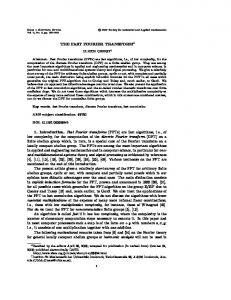
Data storage and data distribution in the parallel FLT algorithm for four processors. The Chebyshev coecients of the intermediate polynomials are stored in four arrays. Array f contains the polynomials Zl2K which are already available at the start of the stage. Array u contains the polynomials Zl2+KK which become available at the end of the stage. Similarly, arrays g and v contain the next higher polynomials Zl2+1K and Zl2+KK+1 , respectively; these arrays are not depicted. Each array is divided into four local subarrays by using the block distribution. Each processor has one subarray. Figure 1.

k 1

K; K ? 1 32 31

2

16 15

3

8 7

Proc(0)

l=1 j = 0; : : : ; 63 l=1 j = 0; : : : ; 31 l=1 j = 0; : : : ; 15

Proc(1)

Proc(2)

l = 33 j = 0; : : : ; 31 l = 33 j = 0; : : : ; 15

l = 17 j = 0; : : : ; 15

Proc(3)

l = 49 j = 0; : : : ; 15

Data structure and distribution of the precomputed data needed in the recurrence with N = 64, M = 8 and p = 4. Data are stored in two two-dimensional arrays Q and R. Each pair of rows in an array stores the data needed for one stage k. Figure 2.

n and rn , for l = 1; M +1; 2M +1; : : :; N ? M +1, The termination coecients ql;m l;m m = 1; 2; : : : ; M ? 2 and n = 0; 1; : : : ; m are stored in a two-dimensional array T of size N=M  (M (M ? 1)=2 ? 1). The coecients for one value of l are stored in row (l ? 1)=M of T. Each row has the same internal structure, as follows. The coecients are stored in increasing order of m. The coecients with the same m are ordered by increasing n. This format is similar to that commonly used to store lower triangular n = 0 or rn = 0, and hence we only need to matrices. For each n and m, either ql;m l;m store the value that can be nonzero. Since this depends on whether n ? m is even or 9

n and rn . Figure 3 illustrates this data odd, we obtain an alternating pattern of ql;m l;m structure. m=1 m=2

m=3

l = 1 r0 q1 q0 r1 q2 r0 q1 r2 q3 l = 9 r0 q1 q0 r1 q2 r0 q1 r2 q3 l = 17 r0 q1 l = 25 r0 q1 l = 33 r0 q1 l = 41 r0 q1 l = 49 r0 q1 l = 57 r0 q1

m=4

m=5

m=6

q0 r1 q2 r3 q4 r0 q1 r2 q3 r4 q5 q0 r1 q2 r3 q4 r5 q6

q0 r1 q2 r3 q4 r0 q1 r2 q3 r4 q5 q0 r1 q2 r3 q4 r5 q6

q0 r1 q2 r0 q1 r2 q3

q0 r1 q2 r3 q4 r0 q1 r2 q3 r4 q5 q0 r1 q2 r3 q4 r5 q6

q0 r1 q2 r0 q1 r2 q3

q0 r1 q2 r3 q4 r0 q1 r2 q3 r4 q5 q0 r1 q2 r3 q4 r5 q6

q0 r1 q2 r0 q1 r2 q3

q0 r1 q2 r3 q4 r0 q1 r2 q3 r4 q5 q0 r1 q2 r3 q4 r5 q6

q0 r1 q2 r0 q1 r2 q3

q0 r1 q2 r3 q4 r0 q1 r2 q3 r4 q5 q0 r1 q2 r3 q4 r5 q6

q0 r1 q2 r0 q1 r2 q3

q0 r1 q2 r3 q4 r0 q1 r2 q3 r4 q5 q0 r1 q2 r3 q4 r5 q6

q0 r1 q2 r0 q1 r2 q3

q0 r1 q2 r3 q4 r0 q1 r2 q3 r4 q5 q0 r1 q2 r3 q4 r5 q6

Proc(0)

Proc(1)

Proc(2)

Proc(3)

Data structure of the precomputed data needed for termination n and rn , for l = with N = 64, M = 8 and p = 4. The coecients ql;m l;m 1; M + 1; 2M + 1; : : :; N ? M + 1, m = 1; 2; : : :; M ? 2, and n = 0; 1; : : :; m n and are stored in a two-dimensional array T. In the picture, rn denotes rl;m n n q denotes ql;m. Figure 3.

The termination stage becomes local if M  N=p, so that the input and output vectors are local. The necessary precomputed data must then also be available locally. This means that each row of T must be assigned to one processor, namely to the processor that holds the subvectors for the corresponding value of l. The distribution N ) achieves this. As a result, the N=M rows of T are distributed T[i; j ] 2 Proc(i div pM in consecutive blocks of rows. 3.3. The Basic Parallel Algorithm Now we formulate our basic parallel algorithm. For this we introduce the following conventions:  Processor identi cation. The total number of processors is p. The processor identi cation number is s, with 0  s < p.  Supersteps. The labels on the left-hand side indicate a superstep and its type: (Cp) computation superstep, (Cm) communication superstep, (CpCm) subroutine containing both computation and communication supersteps. In principle, each superstep ends with an explicit synchronization (In an actual implementation, synchronizations can sometimes be saved). The supersteps are numbered as textual supersteps. Of course, supersteps inside loops are executed repeatedly, even though they are numbered only once.  Indexing. All the indices are global. This means that array elements have a unique index which is independent of the processor that owns it. This enables us to describe variables and gain access to arrays in an unambiguous manner, even though the array is distributed and each processor has only part of it. 10

 Vectors and Subroutine calls. All the vectors (or one-dimensional arrays) are indicated in boldface. To specify part of a vector we write its rst element in boldface, e.g., fj; the vector size is explicitly written as a parameter.  Communication. Communication between processors is indicated using gj Put(pid; n; fi ) This operation puts n elements of vector f , starting from element i, into processor pid and stores them there in vector g starting from element j .  Copying a vector. The operation gj Copy(n; fi) denotes the copy of n elements of vector f , starting from element i, to a vector g starting from element j .  Subroutine name ending in 2. Subroutines with a name ending in 2 perform

an operation on 2 vectors instead of one. For example (fi; gj ) Copy2(n; uk; vl) is an abbreviation for fi Copy(n; uk ) gj Copy(n; vl)  Truncation. The operation f BSP Trunc(s; p; s0; s1; p1; N; K; u) denotes the truncation of all the N=(2K ) polynomials stored in f and u by copying the rst K Chebyshev coecients of the polynomials stored in u into the memory space of the last K Chebyshev coecients of the corresponding polynomials stored in f . A group of p1 processors starting from Proc(s0) work together to truncate one polynomial; s1 with 0  s1 < p1 denotes the local processor number within the group. Note that s0 + s1 = s. When p1 = 1 one processor is in charge of the truncation of one or more polynomials. Algorithm 3 gives a description of this operation. In Fig. 1, this operation is depicted by arrows.  Fast Chebyshev transform. The subroutine BSP FChT(s0; s1; p1; sign; n; f ) replaces the input vector f of size n by its Chebyshev transform if sign = 1 or by its inverse Chebyshev transform if sign = ?1. A group of p1 processors starting from Proc(s0) work together; s1 with 0  s1 < p1 denotes the local processor number within the group. For a group size p1 = 1, this subroutine reduces to the sequential fast Chebyshev transform algorithm. The basic template for the fast Legendre transform is presented as Algorithm 4. At each intermediate stage k, 1  k  log2 N=M , there are 2k?1 independent problems, one for each l. For k  log2 p, there are more processors than problems, so that the 11

Algorithm 3 Truncation using the block distribution. CALL f BSP Trunc(s; p; s0; s1; p1; N; K; u). DESCRIPTION if p1 = 1 thenN for l = s p to (s +1) Np ? 2K step 2K do fl+K Copy(K; ul) else if s1 < p1=2 then fs Np +K Put(s + p21 ; Np ; us Np ) processors will have to work in groups. Each group of p1 = p=2k?1 > 1 processors handles one subvector of size 2K , K = N=2k ; each processor handles a block of 2K=p1 = N=p vector components. In this case, the l-loop has only one iteration, namely l = s0N=p, and the j -loop has N=p iterations, starting with j = s1N=p, so that the indices l + j start with (s0 + s1)N=p = sN=p, and end with (s0 + s1)N=p + N=p ? 1 = (s + 1)N=p ? 1. Inter-processor communication is needed, but it occurs only in two instances:  Inside the parallel FChTs (in supersteps 2, 5, 7). This communication will be discussed separately, in the following subsections.  At the end of each stage (in supersteps 3, 8). For k  log2 p + 1, the length of the subvectors involved becomes 2K  N=p. In that case, p1 = 1, s0 = s, and s1 = 0, and each processor has one or more problems to deal with, so that the processors can work independently and without communication. Note that the index l runs only over the local values sN=p, sN=p + 2K; : : : ; (s + 1)N=p ? 2K , instead of over all values of l. The original stages 0 and 1 of Algorithm 1 are combined into one stage and then N and performed eciently, as follows. First, in superstep 1, the polynomials Z1N , ZN= 2 N ZN= are computed directly from the input vector f . This is possible because the 2+1 N point-value representation of Z1 = TN (f
P1 ) = TN (f
x) needed by the recurrences is the vector of fj
xNj ; 0  j < N , see Subsection 2.1. Note that the values R[i; j ] + Q[i; j ]xNj for i = 0; 1 can be precomputed and stored so that the recurrences only require one multiplication by fj . In superstep 2, polynomials Z0N=2 = f ; Z1N=2 = N=2 = u, and Z N=2 = v are transformed to Chebyshev representation; and then g; ZN= 2 N=2+1 truncated, in superstep 3, in order to obtain the input for stage 2. The main loop works as follows. In superstep 4, the polynomials Zl2K , with K = N=2k and l = 0; 2K; : : : ; N ? 2K , are copied from the array f into the auxiliary array u, where they are transformed into the polynomials Zl2+KK in supersteps 5 to 7. (Similarly, the polynomials Zl2+1K are copied from g into v and then transformed into the polynomials Zl2+KK+1 .) Note that f corresponds to the lower value of l, so 12

Algorithm 4 Basic parallel template for the fast Legendre transform. CALL BSP FLT(s; p; N; M; f ). ARGUMENTS

s: Processor identi cation (0  s < p). p: Number of processors (p is a power of 2 with p  N=2). N : Transform size (N is a power of 2 with N  4). M : Termination block size (M is a power of 2 with M  min(N=2; N=p)). f : (Input) f = (f0; : : :; fN ?1): Real vector to be transformed. (Output) f = (f^0 ; : : :; f^N ?1): Transformed vector. Block distributed: fj 2 Proc(j div Np ).

STAGE 1: (1Cp ) for j = s Np to (s +1) Np ? 1 do gj xNj fj uj (R[0; j ] + Q[0; j ]xNj )fj vj (R[1; j ] + Q[1; j ]xNj )fj CpCm (2 ) BSP FChT2(0; s; p; 1; N; f ; g) BSP FChT2(0; s; p; 1; N; u; v) Cm (3 ) (f ; g) BSP Trunc2(s; p; 0; s; p; N; N=2; u; v) STAGE k: for k = 2 to logk2 N=M do Cp (4 )

(5CpCm ) (6Cp )

(7CpCm ) (8Cm )

K p1 s0 s1

N=2

max(p=2k?1 ; 1) (s div p1)p1 s mod p1 (us Np ; vs Np ) Copy2( Np ; fs Np ; gs Np ) for l = s0 Np to (s0 + 1) Np ? 2pK1 step 2pK1 do BSP FChT2(s0; s1; p1; ?1; 2K; ul; vl) for j = s1 Np to s1 Np + 2pK1 ? 1 do a1 R[2k ? 2; l + j ]ul+j + Q[2k ? 2; l + j ]vl+j a2 R[2k ? 1; l + j ]ul+j + Q[2k ? 1; l + j ]vl+j ul+j a1 vl+j a2 BSP FChT2(s0; s1; p1; 1; 2K; ul; vl ) (f ; g) BSP Trunc2(s; p; s0; s1; p1; N; K; u; v)

STAGE log2 N=MN+ 1: for l = s p to (s +1) Np ? M step M do fl Terminate(l; M; fl; gl)

(9Cp )

13

that in the recurrence the components of f must be multiplied by values from R. In superstep 8, all the polynomials are truncated by copying the rst K Chebyshev coecients of Zl2+KK into the memory space of the last K Chebyshev coecients of Zl2K . The termination procedure (superstep 9) is described separately as Algorithm 5. Algorithm 5 Termination procedure for the fast Legendre transform. CALL Terminate(l; M; f ; g)

INPUT

l: Block identi er. M : Termination block size (M is a power of 2; l mod M = 0). f = (f0; : : :; fM ?1): Chebyshev coecients of polynomial ZlM . g = (g0; : : :; gM ?1): Chebyshev coecients of polynomial ZlM+1. OUTPUT h = (h0; : : :; hM ?1): hi = f^l+i; 0  i < M .

STEPS

h0 f0 h1 g0 b 0 for m = 1 to M ? 3 step1 2 do hm+1 f0T[l; b] + 2 g1T[l; b + 1] hm+2 g0T[l; b + m + 1] + 12 f1 T[l; b + m + 2] for n = 2 to m ? 1 step 2 do hm+1 hm+1 + 12 (fn T[l; b + n] + gn+1 T[l; b + n + 1]) hm+2 hm+2 + 12 (gn T[l; b + n + m + 1] + fn+1 T[l; b + n + m + 2]) hm+2 hm+2 + 12 gm+1 T[l; b + n + m + 3] b b + 2m + 3

3.4. Fast Chebyshev Transform The eciency of the FLT algorithm strongly depends on the FCT algorithm used to perform the Chebyshev transform. There exists a substantial amount of literature on this topic and many implementations of sequential FCTs are available (see e.g. Press et al.16 and Steidl and Tasche19). Parallel algorithms or implementations have been less intensively studied, see Shalaby17 for a recent discussion. In the FLT algorithm, the Chebyshev transforms always come in pairs, which led us to develop an algorithm that computes two Chebyshev transforms at the same time. This algorithm is based on the FCT algorithm 4.4.6 of van Loan21 and the standard algorithm for computing the FFTs of two real input vectors at the same time (see e.g. Press et al.16). The algorithm has the following structure: 1. PACK the two input vectors as one auxiliary complex vector. 14

2. TRANSFORM the auxiliary vector using an FFT 3. EXTRACT the desired Chebyshev transforms from the transformed auxiliary vector. The Chebyshev transforms are computed as follows. Let x and y be the input vectors of length N . We view x and y as the real and imaginary part of a complex vector (xj + i yj ), 0  j < N . Phase 1, the packing of the input data into the auxiliary complex vector z of lenght N is just a simple permutation,  zj = (x2j + i y2j ) (17) zN ?j?1 = (x2j+1 + i y2j+1); for 0  j < N=2: In phase 2, the complex FFT creates a complex vector Z of length N;

Zk =

N ?1 X j =0

zj e

ijk N ;

2

for 0  k < N:

(18)

(Note that we de ne the discrete Fourier transform with a positive sign in the exponent.) Finally, in phase 3 we obtain the Chebyshev transform by  ik  8  1 k > > < x~k = N Re 2 e N (Zk + Z N ?k )   ; for 0  k < N; (19) > > : y~k = k Re ? i e ikN (Zk ? Z N ?k ) N 2 where Nk is the normalization factor needed to get the Chebyshev transform from the cosine transform. The inverse Chebyshev transform is obtained by inverting the procedure described above. The phases are performed in the reverse order, and the operation of each phase is replaced by its inverse. Phase 3 is inverted by packing x~ and y~ into the auxiliary complex vector Z: 8 Z = N (~x + i y~ ); 0 0 < 0 (20) N ik : Zk = e? N ((~xk + i y~k ) + i(~xN ?k + i y~N ?k )) ; for 1  k < N: k In phase 2, an inverse complex FFT is computed, N ?1 X ijk zk = N1 (21) Zj e? N ; for 0  k < N: j =0 The desired transforms are stored as the real and imaginary parts of z respectively, but in a dierent ordering. The inverse of phase 1 is again a permutation.  x2j = Re(zj ) y2j = Im(zj ) (22) ; x2j+1 = Re(zN ?j?1) y2j+1 = Im(zN ?j?1); for 0  j < N=2: 2

2

2

2

15

If we use a radix-4 algorithm21 to perform the FFT, the op count for this FChT2 algorithm is 2:125N log2 N + 8N ? 16 against 2:125N log2 N + 8:25N ? 22 for performing two FChTs one after the other. Theoretically it is only a small improvement although in practice we found the gain to be substantial. An ecient parallelization of this algorithm within the framework of the FLT algorithm involves breaking open the parallel FFT inside the FChT and merging parts of the FFT with the surrounding computations. In the following subsections we give a brief explanation of the parallelization process. 3.5. Fast Fourier Transform The FFT is a well-known method for computing the discrete Fourier transform Eq. (18) of a complex vector of length N in O(N log N ) operations. It can concisely be written as a decomposition of the Fourier matrix FN , FN = AN


A4A2PN ; (23) where FN is an N  N complex matrix, PN is an N  N permutation matrix corresponding to the so-called bit reversal permutation, and the N  N matrices AK are de ned by AK = IN=K BK ; for K = 2; 4; : : : ; N; (24) which is shorthand for a block-diagonal matrix diag(BK ; : : : ; BK ) with N=K copies of the K  K matrix BK on the diagonal. The matrix BK is known as the K  K butter y matrix. This matrix in turn can be written as   I

K= 2 K= 2 : (25) BK = I K=2 ? K=2 Here, the matrix IK=2 is the K=2  K=2 identity matrix and K=2 is the K=2  K=2 diagonal matrix N ? i (26)

K=2 = diag(1; e Ni ; e Ni ; : : : ; e N ): This matrix decomposition naturally leads to an algorithm, which is commonly called the radix-2 FFT .8,21 Performing a Fourier transform on a vector z of length N is equivalent to multiplying it with the Fourier matrix FN . This can best be done by rst permuting and then multiplying the vector successively by all the matrices AK . The multiplications are thus carried out in log2 N stages, each with N=K times a butter y computation. One butter y computation modi es K=2 pairs (zj ; zj+K=2) by adding a multiple of zj+K=2 to zj and subtracting the same multiple. The main choice in developing a parallel FFT is the data distribution for each stage of the computation. It is natural to start with the block distribution, since this renders all butter y computations local, as long as K  N=p. In that case, the butter y matrices are multiplied with a vector block of length K which is completely contained within the local block of the processor, which has length N=p. (Note that 4

2

16

(

2)

blocks are always properly aligned, since the K and N=p are both powers of two.) As a result, the rst log2 N ? log2 p stages are local. To nish the computation, it is convenient to use the cyclic distribution, which is formally de ned as follows. De nition 3.2. (Cyclic distribution). Let z be a vector of size N . We say that z is cyclically distributed over p processors if for all j , the element zj is stored in Proc(j mod p) and has local index j 0 = j div p. For the cyclic distribution, the butter ies are local provided K  2p. In that case, the pair of components to be modi ed is at distance K=2  p and hence p is a divisor of K=2; therefore both components j and j + K=2 are on the same processor. As a result, the last log2 N ? log2 p stages are local. Our approach for the parallel FFT is to start with the block distribution and after log2 N ? log2 p stages switch to the cyclic distribution. (Note that this is equivalent to permuting the vector z.)p This can be done if log2 N ? log2 p  21 log2 N (i.e., p p  N ). If, however, p > N , the use of the block distribution is exhausted before we can use the cyclic distribution. In that case, other intermediate distributions must be used, see McColl.14 We perform the inverse transform by reversing the stages of the algorithm and inverting the butter ies, instead of taking theimore common approach of using the same algorithm, but replacing the powers of e N by their conjugates and multiplying by an rescaling factor. This choice enables us to eliminate certain permutations, see the next subsection. 3.6. Optimization of the Main Loop Breaking open the FChT module allows us to radically reduce the amount of communication involved in the parallel FLT algorithm. As a consequence, the amount of local copy operations and computations is also reduced, but to a lesser extent. The original modular parallel algorithm for the p FChT of two vectors x and y of size N block distributed over p processors, p  N , has the following structure: 1. PACK vectors x and y as the auxiliary complex vector z by permuting them using Eq. (17). 2. TRANSFORM vector z using an FFT of size N . (a) Perform a bit-reversal permutation in z. (b) Perform the butter ies of size 2; 4; : : : N=p. (c) Permute z to the cyclic distribution. (d) Perform the butter ies of size 2N=p; 4N=p; : : : ; N . (e) Permute z to the block distribution. 3. EXTRACT the transforms from vector z and store them in vectors x and y. (a) Permute z to put components j and N ? j in the same processor. (b) Compute the new values of z using Eq. (19). (c) Permute z to block distribution and store the result in vectors x and y. 2

17

0

4

8

12

16

20

24

28 Proc(0)

(a)

Proc(1) Proc(2)

(b)

Proc(3)

(a) Cyclic distribution and (b) zig-zag cyclic distribution for a vector of size 32 distributed over 4 processors.

Figure 4.

In our optimized version where modularity p is not an issue, we restrict the number of processors slightly further to p  N=2 and permute the vector z from block distribution to a slightly modi ed cyclic distribution de ned as follows. De nition 3.3. (Zig-zag cyclic distribution). Let z be a vector of size N . We say that z is zig-zag cyclically distributed over p processors if for all j , the element zj is stored in Proc(j mod p) if j mod 2p < p and in Proc(?j mod p), if j mod 2p  p and has local index j 0 = j div p. With this distribution both the components j and j + K=2, with 2N=p  K  N , needed by the butter y operations and the components j and N ? j needed by the extract operation are in the same processor; thus we can avoid the permutations performed in phases (2e) and (3a) above. The same happens, though in reversed order, in the pack/transform phases of the parallel inverse FChT. Figure 4 illustrates the cyclic and zig-zag cyclic distributions. By giving up the block distribution in the main loop of the FLT algorithm and instead maintaining the vectors fl; gl ; ul; and vl of size 2K in the zig-zag cyclic distribution of p1 processors, we can also save the permutations to convert from zig-zag cyclic to block distribution in phase (3c) of the FChT and from block to zig-zag cyclic distribution in the corresponding phase of the inverse FChT. To achieve this we replace the truncation operation, Algorithm 3, by a new truncation operation, namely the redistribution of vectors fl ; gl; ul ; and vl, now of size K , from the zig-zag cyclic distribution with p1 processors to the zig-zag cyclic distribution with p1=2 processors, storing the lower halves of vectors ul and vl in the upper halves of vectors fl; gl . Note that the initialization step must also be modi ed in order to give the input vectors of stage 2 in the zig-zag cyclic distribution of p=2 processors. Furthermore, the optimized algorithm avoids the packing (1) and bit-reversal (2a) in the FChT just following the recurrence and their corresponding inverses in the inverse FChT preceding the recurrence. This is done by storing the recurrence coef cients permuted by the packing (1) and bit-reversal (2a) permutations. This works because the last two permutations form the inverse of the rst two, so that the auxiliary vector z is in the same ordering immediately before and after the permutations. After all the optimizations, the total communication and synchronization cost is N (6 p log2 p + 2 Np )g + (3 log2 p + 1)l. This means that we reduced communications and synchronizations by more than a factor of two. (The basic algorithm has a communication and synchronization cost of 14 Np log2 p g + 7 log2 p l.) 18

Since we do not use the upper half of the Chebyshev coecients computed in the forward transform, we can alter the algorithm to avoid computing them. To make our code more competitive we used a modi ed radix-2 algorithm. Wherever possible we take pairs of stages A2K AK together and perform them as one operation. The butter ies have the form B2K (I2 BK ), which is a 2K  2K matrix consisting of 4  4 blocks, each a K=2  K=2 diagonal submatrix. (This matrix is a symmetrically permuted version of the radix-4 butter y matrix.21) This approach gives the eciency of a radix-4 FFT algorithm, and the exibility of treating the parallel FFT within the radix-2 framework; for example, it is possible to redistribute after any number of stages, and not only after an even number of them. Supposing N and p are powers of 4, i.e., we can always take pairs of stages together, the total cost of the optimized algorithm is:

TFLT = 4:25 Np (log2 N )2 +26:25 Np log2 N ? (4:25(log2 M )2 +26:25 log 2 M + M ) Np +  N N 6 p log2 p + 2 p g + (3 log2 p + 1) l: 4. Experimental Results In this section, we present results on the accuracy and scalability of the implementation of the Legendre transform algorithm for various sizes N . We set M = 2, i.e., no early termination. We implemented the algorithm in ANSI C using the BSPlib communications library. The test runs were made on a Cray T3E with up to 64 processors, each having a theoretical peak speed of 600 M op/s. We tested the accuracy of our implementation by measuring the error obtained when transforming an arbitrary input vector f with elements uniformly distributed between 0 and 1. Table 1 shows the relative errors obtained for various problem sizes. The relative errors were computed via the expression

jj^f ? ^fjjmax ; jj^fjjmax

where ^f is the exact transform (computed by a quadruple precision direct Legendre transform) and ^f the FLT; jj
jjmax indicates the max norm.

Table 1 Estimated relative errors for the FLT algorithm. N 1024 8192 65536

relative error 7:8  10?14 1:3  10?13 2:6  10?12 19

We tested the scalability of our parallel implementation using our sequential implementation as basis for comparison. Though we broke open the modules of the algorithm, it is still possible (with a certain amount of work) to replace the FFT subroutine by a highly optimized or even a machine speci c, assembler coded, FFT subroutine in both the sequential and the parallel versions. This would yield an even faster program. Table 2 shows the timing results obtained for the sequential and parallel versions executed on up to 64 processors. It is better to analyze these results in terms of absolute speedups, S abs = t(seq)=t(p), i.e., the time needed to run the sequential program divided by the time needed to run the parallel program on p processors. Our goal is to achieve ratios as close to p as possible. Figure 5 shows the performance ratios obtained for various input sizes on up to 64 processors.

Table 2 Timing data for BSP FLT on a Cray T3E. All times are given in milliseconds. N seq p = 1 p = 2 p = 4 p = 8 p = 16 p = 32 p = 64 512 1:71 1:89 1:23 0:80 0:58 0:61 { { 1024 3:95 4:36 2:70 1:57 1:08 0:84 { { 8192 50:60 65:70 33:60 17:40 8:71 5:16 3:38 3:34 65536 1130:? 1250:? 664:? 336:? 162:? 71:10 36:10 20:30 FLT speedups on the CRAY T3E 64.0 16.0

56.0

speedup (t(seq)/t(p))

48.0

12.0 8.0 4.0

40.0 0.0

1 2

4

8

16

32.0 24.0 16.0 N=512 N=1024 N=8192 N=65536 ideal

8.0 0.0

12 4

Figure 5.

8

16

32 number of processors (p)

64

Scalability of the program BSP FLT on a Cray T3E 20

It is clear that for a large problem size (N = 65536) the speedup is close to ideal, e.g., S abs = 56 on 64 processors. For smaller problems, reasonable speedups can be obtained using 8 or 16 processors, but beyond that the communication time becomes dominant. 5. Conclusions and Future Work As part of this work, we developed and implemented a sequential algorithm for the discrete Legendre transform, based on the Driscoll-Healy algorithm. We believe this implementation to be quite competitive for large problem sizes. Its complexity O(N (log2 N )2) is considerably lower than the O(N 2) matrix-vector multiplication algorithms which are still much in use today for the computation of Legendre transforms. The new algorithm is a promising approach for compute-intensive applications such as weather forecasting. The main aim of this work was to develop and implement a parallel Legendre transform algorithm. Our experimental results show that the performance of our parallel algorithm scales well with the number of processors, for medium to large problem sizes. The overhead of our parallel program consists mainly of communication, and this is limited to three redistributions of the data vector in each of the rst log2 p stages of the algorithm. Two of these redistributions are already required by an FFT and an inverse FFT, indicating that this is close to optimal. Our parallelization approach was rst to derive a basic algorithm that uses block and cyclic data distributions, and then to optimize this algorithm by removing permutations and redistributions wherever possible. To facilitate this we proposed a new data distribution, which we call the zig-zag cyclic distribution. Within the framework of this work, we also developed a new algorithm for the simultaneous computation of two Chebyshev transforms. This is useful in the context of the FLT because the Chebyshev transforms always come in pairs, but such a double fast Chebyshev transform (and the corresponding double fast cosine transform) also has many applications in its own right. Our algorithm has the additional bene t of easy parallelization. We view the present FLT as a good starting point for the use of fast Legendre algorithms in practical applications. However, to make our FLT algorithm directly useful in such applications further work must be done: an inverse FLT must be developed, the FLT must be adapted to the more general case of the spherical harmonic transform, and alternative choices of sampling points must be made possible. 6. Acknowledgements We thank CAPES, Brazil, for supporting Inda with a doctoral fellowship and NCF, The Netherlands, for funding the computer time on the Cray T3E. 21

7. References 1. N. Ahmed, T. Natarajan, and K. Rao, IEEE Trans. Comput. 23 (1974) 90. 2. B. Alpert and V. Roklin, SIAM J. Sci. Statist. Comput. 12 (1991) 158. 3. S. Barros and T. Kauranne, Parallel Computing 20 (1994), 1335. 4. P. Barrucand and D. Dickinson, On the Associated Legendre Polynomials, in Orthogonal Expansions and Their Continuous Analogues, (Southern Illinois University Press, Carbondale, IL, 1968). 5. S. Belmehdi, J. Comput. Appl. Math. 32 (1990) 311. 6. R. H. Bisseling, in Lecture Notes in Computer Science 1196 (Springer-Verlag, Berlin, 1997), p. 46. 7. G. L. Browning, J. J. Hack and P. N. Swarztrauber, Mon. Wea. Rev. 117 (1989) 1058. 8. J. W. Cooley and J. W. Tukey, Math. Comp. 19 (1965) 297. 9. J. Driscoll and D. Healy, Adv. in Appl. Math., 15 (1994) 202. 10. J. R. Driscoll, D. Healy, and D. Rockmore. SIAM J. Comput. 26 (1997) 1066. 11. D. Healy, S. Moore, and D. Rockmore, Eciency and Stability Issues in the Numerical Computation of Fourier Transforms and Convolutions on the 2-Sphere, (Technical Report PCS-TR94-222, Dept. of Math. and Com. Sci., Dartmouth College, NH, 1994). 12. J. M. D. Hill, B. McColl, D. C. Stefanescu, M. W. Goudreau, K. Lang, S. B. Rao, T. Suel, T. Tsantilas, and R. H. Bisseling, Parallel Computing 24 (1998) 1947. 13. D. K. Maslen, A Polynomial Approach to Orthogonal Polynomial Transforms, (Preprint MPI/95-9, Max-Planck-Institut fur Mathematik, Bonn, Germany, 1995). 14. W.F. McColl, Future Generation Computer Systems, 12 (1996) 265. 15. S. Orszag, in Science and Computers, ed. G. Rota, (Academic Press, NY 1986), p. 23. 16. W. Press, S. Teukolsky, W. Vetterling and B. Flannery, Numerical Recipes in C: The Art of Scienti c Computing, second edition, (Cambridge University Press, Cambridge, UK, 1992). 17. N. Shalaby, Parallel Discrete Cosine Transforms: Theory and Practice, (Technical report TR-34-95, Center for Research in Computing Technology, Harvard University, Cambridge, MA, 1995). 18. N. Shalaby and S.L. Johnsson, Hierarchical Load Balancing for Parallel Fast Legendre Transforms, (8th SIAM Conference on Parallel Processing for Scienti c Computation, 1997). 19. G. Steidl and M. Tasche, Mathematics of Computation, 56 (1991) 281. 20. L. Valiant, Communications of the ACM 33 (1990) 103. 21. C. Van Loan, Computational Frameworks for the Fast Fourier Transform, (Society for Industrial and Applied Mathematics, SIAM, Philadelphia 1992). 22