Sep 23, 1996 - algorithms would also be superior in a shared-everything environment. ... of the low execution time cost and space overhead for creating a task ...
Parallel Hash-Based Join Algorithms for a Shared-Everything Environment� T. Patrick Martiny, Per-� Ake Larsonzand Vinay Deshpande September 23, 1996 Abstract
We analyze the costs, and describe the implementation, of three hashed-based join algorithms for a general-purpose shared-memory multiprocessor. The three algorithms considered are the Hashed Loops, GRACE and Hybrid algorithms. We also describe the results of a set of experiments which validate the cost models presented and demonstrate the relative performance of the three algorithms.
Index Terms algorithms, cost models, parallel systems, query processing, relational database systems.
1 Introduction The LauRel project [10] is aimed at extending current relational database technology in three areas: data modelling, exploitation of parallelism, and structuring of the stored database. As part of this project, we are building a prototype database system which runs on a general-purpose shared-memory multiprocessor system. A key objective of this implementation is to exploit the parallelism o�ered by the underlying architecture. One of the ways to help achieve this objective is to develop e�cient parallel algorithms to perform the basic operations used in the query processing module of such a database system. Once these parallel algorithms have been developed, reliable and realistic cost models are required for query optimization purposes. The formulation of these cost models is more complex in a This work was supported by the ITRC: Information Technology Research Centre, Ontario. P. Martin is with the Department of Computing and Information Science, Queen's University, Kingston, Ontario, CANADA K7L 3N6. z P. Larson is with the Department of Computer Science, University of Waterloo, Waterloo, Ontario, CANADA N2L 3G1. � y
1
parallel environment because resources such as the number of processors and the number of disks are now parameters in the models. In this paper, we analyze the costs, and describe implementations, of three popular hash-based join algorithms for a shared-memory multiprocessor system. The three algorithms studied are the Hashed Loops, GRACE and Hybrid algorithms. Cost models of the three algorithms are presented and then validated with respect to the implementations. The remainder of the paper is structured in the following manner. Section 2 presents a brief survey of related work. Section 3 describes the Query Processing Environment of the LauRel system. We outline the system architecture, and the programming model used in the algorithms' implementation. Section 4 discusses our approach to performing the cost analysis. Section 5 describes the implementation of the algorithms and outlines their cost models. Section 6 presents the results of a set of experiments carried out to validate the cost models and to examine the performance of the algorithms. Finally, Section 7 contains our conclusions.
2 Related Work The join operation is one of the most frequently-used, and most expensive, operations in a relational system. It has therefore received a great deal of attention and algorithms for a variety of environments have been proposed. Recent work has resulted in a number of attractive alternatives to the traditional nested loops and sort-merge algorithms. One environment where join algorithms have been studied is machines with large main memories [6, 19]. Another popular environment for this work has been distributed-memory, or shared-nothing multiprocessor systems [1, 3, 7, 9, 12, 16, 20]. In most of these studies it has been found that, for the join of large sequential les, hash-based algorithms outperform the nested loops and the sort-merge algorithms. In the case of large main memory, the hash-based algorithms were able to take full advantage of the memory to reduce the amount of I/O required. In the case of a multiprocessor system, the hash-based algorithms are easily parallelized and the work involved can be easily partitioned among the available processors. 2
Our environment, which is a shared-memory multiprocessor, or shared-everything, system, has features in common with both of the previous environments. We have one large main memory which must be used to its full advantage | the performance of hashed-based algorithms is very sensitive to the amount of main memory available. We also have the advantage of parallel processors so that the work of the join can be partitioned. These similarities led us to expect that hash-based algorithms would also be superior in a shared-everything environment. The key di�erence between the shared-nothing and shared-everything environments is the replacement of communication costs in a shared-nothing system by the cost of contention for sharedmemory in a shared-everything system. This di�erence leads to very di�erent implementations of the same algorithms. Work on database systems in the shared-everything environment has not been as wide-spread as in the shared-nothing environment. The Volcano project [8] has goals similar to our LauRel project and is also implemented on a general-purpose shared-memory multiprocessor. Volcano deals with the standard relational model while LauRel has a nested relational model. Qadah and Irani [14] have studied join algorithms for a specialized shared-memory database machine, and Lu, Tan and Shan [11] have also developed cost models for a set of hash-based join algorithms on a general purpose shared-memory multiprocessor. The latter work is most closely related to the research described in this paper. The main contribution of our work beyond these other research e�orts is the validation of our cost models with respect to actual implementations of the algorithms.
3 Query Processing Environment 3.1 Multiprocessor System Architecture The LauRel system, as mentioned earlier, is being designed to run on a general-purpose sharedmemory multiprocessor system. The machine used is a Sequent Symmetry [17]. The architecture of the system, which is shown in Figure 1, consists of a number of processors, memory modules, disk controllers, and other I/O controllers, which are all linked together by a high-speed bus. Our machine is currently con gured with ten processors, thirty-two MBytes of main memory, and two 3
architecture diagram goes here Figure 1: Multiprocessor System Architecture I/O controllers, each with two channels and one disk per channel. The processors operate on a \peer" basis, that is, all processors are considered equal, and they all have access to the shared memory and I/O units. A process runs on any available processor until it blocks or is interrupted. There is a single copy of the operating system kernel and any processor can execute kernel functions. The shared memory provides an e�cient means of communication among the processors and access to shared data structures is controlled by an e�cient locking mechanism. The system architecture places a number of constraints on how we implement the join algorithms. First, the number of processors in this kind of system is relatively small (the Sequent Symmetry has a maximum of 32 processors) when compared to other architectures so the partitioning of the work must be at a coarse level. Second, the use of shared memory for the major data structures introduces the need to synchronize access to these data structures. The shared memory is a source of contention among the processors and any implementation must attempt to minimize this contention. Third, because of the increased processing capacity, database computations run a strong risk of being I/O-bound. An implementation must therefore make maximum use of the available parallelism in the disk subsystem and of the available main memory in order to reduce the amount of I/O performed.
3.2 The Programming Model We have adopted a programming model based on light-weight tasks (hereafter referred to as tasks) with an unlimited degree of parallelism. These tasks are implemented using the �System, which was developed to provide light-weight concurrency on uniprocessor and multiprocessor hardware running the UNIX 1 operating system [5]. The �System uses a shared-memory model of concurrency 1
UNIX is a registered trademark of AT&T Bell Laboratories
4
and provides mechanisms to create tasks within the shared memory, to synchronize execution of the tasks and to facilitate communication between the tasks. A task is a program component with its own thread of control which is scheduled separately and independently from threads associated with other tasks. The tasks are light-weight because of the low execution time cost and space overhead for creating a task and the many forms of communication which are easily and e�ciently implemented for them [5]. Tasks are run on one or more virtual processors . A virtual processor is conceptually a hardware processor that executes tasks but is actually a UNIX process that is subsequently scheduled for execution on the physical processors by the underlying operating system. Thus the �System is not in direct control of the processors but controls the scheduling of tasks on active virtual processors. The �System uses a single task queue and multiple servers, that is, a task in the ready state will be executed by the rst available processor. This automatically balances the load of the system. The �System has its own �Kernel and does not depend upon the UNIX kernel to perform context switches between tasks. This provides a signi cant decrease in execution and communication overhead compared with standard UNIX processes. In some cases the improvement is two orders of magnitude. As well, the only limiting factor on the number of active tasks in a single program is the amount of memory available to that program. An important advantage of this programming model is that tasks provide a way of separating the \logical" and \physical" resources. This allows programs to be written and executed without having to know exactly what physical resources will be available. It also allows for sharing of resources at the system level, that is, applications running under the �System do not monopolize system resources. A second advantage of this approach is that tasks allow both data partitioning and functional partitioning. Functional partitioning means that individual operations can be written as separate tasks and then executed in parallel. Data partitioning means that the data can be split into several streams which can then be processed in parallel. Our join implementations take advantage of both types of parallelism. A third advantage of this approach is that the �System provides automatic load balancing. 5
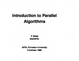
�Kernel Overhead table goes here Table 1: �Kernel Overhead The single task queue ensures maximum CPU utilization by assigning any waiting tasks to the rst available processor. A disadvantage of our programming model is the additional overhead required to manage and synchronize tasks. However, investigation by Buhr and Stroobosscher [5] indicates that this additional overhead is not unreasonable given the above advantages. Table 1 shows the overhead involved in the three most common �System operations in our code, namely task creation and deletion, task context switch, and P/V on a semaphore followed by a context switch. These timings were taken on a Sequent Symmetry S27 running 16MHz i386 processors.
4 Approach to Cost Analysis Each algorithm is composed of a number of phases , where each phase is, in turn, made up of a set of functions. The phases of an algorithm are executed sequentially while the functions within a phase can be performed in parallel. An execution of an algorithm may require the work of one or more phases to be performed in several passes where each pass performs the phases on a portion of the data. We chose to compare the performance of the algorithms with respect to response time since one of the main objectives of this work is to measure the degree to which the di�erent algorithms can exploit the available parallelism. Response time may not be the best criterion, however, for query optimization in a real system. Reducing response time in a parallel system is usually achieved by dedicating a larger amount of resources (CPU, memory, disks) to the transaction but this results in the delay of the other active transactions and a decrease in the overall system throughput. A more appropriate criterion suggested by Pirahesh et. al. [13] is to maximize the use of given limited resources to minimize the response time up to a threshold. This threshold is de ned as that response time below which minimization is not signi cant. 6
The two main components of the cost of executing a join are the processing and the disk I/O. We do not consider any other costs, such as the cost of communication with the user, in our models. We assume that the processing is always evenly distributed among the available processors so that elapsed processing time for an operation on p processors is T=p if T is the elapsed time of the operation run on a single processor. Similarly, if data is spread across d parallel disks, the transfer rate for the data is IO=d if IO is the transfer rate for a single disk. Most of the previous analyses of join algorithms [1, 6, 19, 20] have assumed that there is no overlap between processing and disk I/O. Response time has been calculated as the sum of the processing and the I/O times. It is important to account for this overlap, however, in order to arrive at a more realistic cost estimate and to more cost-e�ectively allocate resources to a query. For example, it would be wasteful to allocate more CPUs to an I/O-bound operation than the minimum number necessary to keep up with the data rate. The work described in Richardson, Lu and Mikkilileni [15] and in Lu, Tan and Shan [11] are exceptions and try to represent the overlap. We ignore any processing related to a disk access so that I/O tasks have no associated processing cost. We also assume that if more than one le is being read or written during a phase then these les are stored on independent sets of disks so that their I/O overlap and the I/O time for the phase is just the maximum of the di�erent I/O times. We assume perfect overlap between the processing and I/O components of a phase of an algorithm so that the response time for phase i, Ti , is
Ti = max(TCPUi; TIOi ) where TCPUi is the processing time, and TIOi is the I/O time, of phase i. The total response time for an algorithm with n phases is
T=
n X i=1
Ti
A second important aspect of our cost models is the representation of the possible contention among processors for locations in the shared memory. Contention can occur between two or more processors whenever they wish to write to the same memory location at the same time. This means 7
that shared variables or data structures must be guarded by some kind of lock and access to them synchronized. Whenever a processor wishes to access a memory location that is already locked then that processor is forced to wait. We de ne a contention point to be a point in the execution of a task where contention with other concurrent tasks can occur. Thus, representing contention in our cost model involves identifying each of the contention points and attributing a cost to the average delay encountered at that point. For example, a contention point in the Hashed Loops algorithm occurs whenever a build task must acquire a new bu�er of R-tuples. If the cost of acquiring this bu�er, ignoring contention, is tbuf , then the estimated cost, with contention is
tbuf � (1 + �) where � is the expected number of other tasks also at that contention point. There are two kinds of contention points in our algorithms: 1. We say that a contention point is single-path if all active tasks2 with that contention point must acquire a single lock at that point. For example the lock associated with the pointer to the head of a queue of bu�ers is a single-path contention point. 2. We say that a contention point is multiple-path if all active tasks with that contention point acquire one of a set of locks at that point. For example, the set of locks associated with the entries in the hash table is a multiple-path contention point. When inserting a tuple into the table the lock required, and hence the path taken, by a task is determined by the tuple currently being processed. We model multiple-path contention with the same technique as described by Lu, Tan and Shan [11]. We formulate the problem of estimating the degree of interference at a multiple-path contention point as follows: We equate the terms \active tasks" and \processors" in this discussion since, for the analysis, we assume there is always the maximum number of any kind of task active, i.e. one task per processor 2
8
Given kRk tuples and H possible paths (1 < H � kRk), if p of the tuples (one per processor) are selected at random (p < kRk ? kRk=H ), nd the expected number of paths with at least one processor. This formulation is similar to the problem of characterizing the number of granules accessed by a transaction. A solution to this problem was given by Yao [21]. Using Yao's theorem we estimate the number of paths followed ( y ) by p kRk � D ? i + 1 Y y =H� 1? i=1 kRk ? i + 1
!
where D = 1 ? 1=H . We estimate the expected number of processors on a path at a multiple-path contention point by
Y (kRk; H; p) = yp
We approximate the number of processors interfering at a single-path contention point simply by
p. This approximation is pessimistic since it assumes all active processors will interfere at a singlepath contention point. However, most of the single-path contention points occur at interface points to I/O tasks so an I/O-bound computation is likely to have all processors waiting at these points. We tried other more complicated representations but did not achieve any better approximations to the actual execution times of the algorithms. Contention points are represented in the cost models by � symbols. The cost models used in our analysis are described in a notation similar to that used by Shapiro [19]; it is summarized in Appendix A. The parameter values used for the models are given in Appendix B. The models assume a uniform distribution of join attribute values across the relations and ignore the possibility of table or bucket over ow. The e�ect of this assumption is examined in some of the experiments of Section 6 where non-uniform distributions are used.
9
5 Hash-Based Join Algorithms The basic approach of all hash-based algorithms to joining two relations R and S is to build a hash table on the join attributes of one relation, say R, and then to probe this table with the hash values of the join attributes of tuples from the other relation S .
3
The result tuples are then formed by
combining the matching tuples from R and S . Each algorithm is implemented as a series of phases. Each function performed within a phase is implemented by a set of identical tasks. Performing the functions of a phase in parallel is an instance of functional partitioning and using several identical tasks to perform a single function is an instance of data partitioning. The completion of each phase is a synchronization point in the implementation. It is usually the case that the amount of memory available is smaller than either of the relations, so the algorithms must perform the join in several passes. In each pass, a portion of R is read into memory and a hash table built for those tuples, then all or a portion of S is processed against that tuple. The key di�erences among the three algorithms discussed below have to do with how the portions of R and S are determined. The CPU costs for a type of task in a given phase are expressed in the cost models as the amount of processing required per block of input data to that type of task times the average number of blocks processed per task. We assume that, if we have p processors, then we always have p instances of each type of processing task so the CPU costs for a phase is just the sum of the task costs. Disk I/O is performed by a set of read and write tasks. The bu�er space for a relation is managed by a pair of queues, for full and empty bu�ers respectively. Each bu�er holds one disk block. During input, a read task takes one or more bu�ers from an empty queue, lls them with tuples, and adds them to a full queue. Full bu�ers are removed from the full queue by a processing task and the used bu�er is later returned to the empty queue. During output, when an output bu�er becomes full it is placed in a full queue. A write task takes one or more bu�ers from a full queue, writes the data to disk, and then adds those bu�er to a queue of empty bu�ers. We will assume that the size of relation R, with respect to both number of tuples and number of blocks, is always less than the size of relation S . 3
10
Hashed Loops pseudo-code goes here Figure 2: Hashed Loops Algorithm
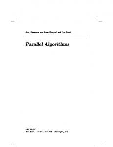
5.1 Hashed Loops The Hashed Loops algorithm is a variation of the traditional nested loops join algorithm [3]. The algorithm is composed of two phases which we call the build and join phases. The number of passes required in an execution of the algorithm is dependent upon the size of the outer relation
R compared with the amount of available memory. Each pass reads as many tuples of R as will t into main memory and builds a hash table for this set of tuples. Each tuple of relation S is then processed against this hash table and matches are written to the result le. The number of passes can be approximated by
� Rj � A = jM
A pseudo-code description of the Hashed Loops algorithm is given in Figure 2. During the build phase of the algorithm, read tasks read, in parallel, a much of R as will t into the available bu�er space. At the same time, a set of parallel build tasks create a hash table for this portion of R by taking the data a block at at time, hashing each tuple on its join attribute, and then inserting a pointer to that tuple into the appropriate location in the table. The hash table is a shared data structure and so access by the build tasks must be synchronized. The hash tables are structured such that there is a lock on every entry in the table. This approach to synchronizing access to the table results in very little contention. Insertion into the table involves locking the entry, and if that entry is empty, then placing the tuple pointer in that entry. If the entry is not empty then it is the start of a chain of pointers to tuples that hash to the same value and the new tuple pointer is placed at the head of the chain. The costs for Phase 1 are estimated by the following:
TCPU1 = jRp j � (bfrR � (thash + tinsert � �1 ) + tbuf � �2 ) TIO1 = jRj � ERDseq 11
Contention for hash table slots while the table is being created is modelled by �1 = Y (kRk=A; H; p). We assume that the cardinality of the range of join attribute values is larger than H . If this is not the case then the cardinality should be used in �1 in place of H since not all of the entries in the table will be used. Contention at the input bu�er queue is modelled by �2 = p. In the second, or join, phase, the read tasks read all of S in parallel, into the available bu�er space for S . In parallel, a set of join tasks take blocks of S as they become available, hash each tuple in the block on its join attribute, probe the hash table for matches, and then write any result tuples to an output bu�er. The join tasks are not required to lock a hash table entry since they only read the table. When a match is found, a join task locks an output bu�er pointer to obtain space in the output bu�er and then copies the matching tuples to the output bu�er. The lock on the bu�er pointer is held only long enough to acquire space to place the result. It is not held during the copying of the tuples. When a join task nishes processing all the tuples in a block it places the block on the empty queue for reuse by the read tasks. A parallel set of write tasks take the output bu�ers as they become full and write the result tuples back to disk. The costs for Phase 2 are represented as follows:
TcpuS = A � jSp j � (bfrS � (thash + pb � tprobe ) + 2 � tbuf � �3 ) j � (bfr � bytes � t + 2 � t � � ) TcpuRS = jRS RS RS copy 3 buf p TCPU2 = TcpuS + TcpuRS TreadS = A � jS j � ERDseq TwriteRS = jRS j � EWTseq TIO2 = max(TreadS; TwriteRS ) TcpuS is the cost of comparing the tuples of the S relation with each of the A hash tables constructed and TcpuRS is the cost of moving result tuples to the output bu�er. pb is the expected number of probes required with a table search. Contention at the full and empty queues for the S 12
GRACE pseudo-code goes here Figure 3: GRACE Algorithm bu�ers and for the result bu�ers are represented by �3 = p. The times to read S and write the result are given by TreadS and TwriteRS , respectively.
5.2 GRACE The GRACE algorithm [9] has four separate phases. The rst two phases \partition", R and S into disjoint subsets, say R1 ; R2 ; :::; RB and S1 ; S2 ; :::; SB . The value B is chosen such that each partition from R ts into main memory. The partitioning is done by hashing on the join attribute value, so that only corresponding partitions need to be considered for the join. After the partitioning phase, the Hashed-Loops algorithm is applied to the corresponding partitions. Some implementations of the algorithm proceed by creating many partitions, so that each partition will be small. Then at the next stage, as many partitions of R as will t into memory are brought in for the hashedloops stage. This technique is known as bucket tuning. A psedo-code description of the GRACE algorithm is given in Figure 3. There are two restrictions which dictate the minimum amount of available memory required by our implementation. First, each of the partitions of R must t into the available memory during the build phase of the execution, that is, � Rj � M � jB
Second, we use double bu�ering for each of the buckets to ensure as much overlap as possible between the processing and I/O components of the phase. This means that �M � B= 2
13
Combining these two facts we have the requirement that q
M � 2 � jRj
p
This required minimum amount of memory is larger by a factor of 2 than other reported minimums but, given that we can use double bu�ering during the partitioning, we feel this is a justi able expense. We use any extra memory to create a larger number of buckets, each with fewer tuples (on average) and then use bucket tuning to combine these smaller buckets into memory size buckets during the second phase. The \partition" phases are implemented with parallel sets of read tasks which read the original relations, write tasks which write out the buckets, and partition tasks which take a block of input at a time and assign tuples from that block to a bucket using a hash function. The partition tasks acquire space for a tuple in the appropriate bu�er by locking a bucket pointer and incrementing it. They then move the tuple to the saved location. The cost to partition R is estimated by the following:
TCPU1 = jRp j � (bfrR � (thash + bytesR � tcopy + tbuf � �4 ) + 2 � tbuf � �5 ) TreadR = jRj � ERDseq TwriteRi = B � jRi j � EWTrand TIO1 = max(TreadR; TwriteRi) The contention at the bu�ers for the B buckets is represented by �4 = Y (kRk; B; p) and contention at the R input queues is given by �5 = p. TreadR and TwriteRi are, respectively, the time to read R and the time to write the buckets R1 ; :::; RB . Random writes are assumed since we cannot predict when a bu�er for a particular bucket will become full. We also assume that buckets are written so that they can be read back sequentially in the subsequent phases.
14
S is partitioned in exactly the same manner as R. The cost equations are as follows: TCPU2 = jSp j � (bfrS � (thash + bytesS � tcopy + tbuf � �6) + 2 � tbuf � �7 ) TreadS = jS j � ERDseq TwriteSi = B � jSi j � EWTrand TIO2 = max(TreadS; TwriteSi) The contention at the bu�ers for the B buckets is represented by �6 = Y (kS k; B; p) and contention at the S input queues is given by �7 = p. TreadS and TwriteSi are, respectively, the time to read
S and the time to write the buckets S1 ; :::; SB . The next two phases of the GRACE algorithm correspond to the build and join phases of the Hashed Loops algorithm. They are implemented by running B passes of Hashed Loops, as described above, for corresponding pairs of R and S buckets. The cost of building the hash tables for the partitions of R is estimated as follows:
TCPU3 = B �pjRi j � (bfrR � (thash + tinsert � �8 ) + tbuf � �9) TIO3 = B � jRi j � ERDseq Contention at the hash table entries is modelled by �8 = Y (kRi k � btf; H; p), where btf is a factor to account for bucket tuning. Contention at the input bu�ers queues is represented by �9 = p. The cost of probing each hash table with the corresponding partition of S is given by the following:
TCPU4 = B �pjSi j � (bfrS � (thash + pbi � tprobe) + 2 � tbuf � �10 ) + jRS j � (bfr � bytes � t + 2 � t � � ) RS RS copy 10 buf p TreadSi = B � jSi j � ERDseq TwriteRS = jRS j � EWTseq TIO4 = max(TreadSi; TwriteRS ) 15
Hybrid pseudo-code goes here Figure 4: Hybrid Algorithm Contention at the input and result bu�er queues is given by �10 = p. The times to read the S buckets and write the results are given by TreadSi and TwriteRS respectively.
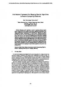
5.3 Hybrid The Hybrid algorithm [6] is a variation of the GRACE algorithm. During the partitioning phase, instead of using extra memory to increase the number of buckets, it introduces an R0 bucket and builds a hash table for it. The relation R is therefore partitioned into B +1 buckets, R0 ; R1 ; : : : ; RB . Bucket R0 is kept in memory, and only partitions 1; : : : B are written out to disk. When S is partitioned, any tuples hashing to the corresponding S0 are immediately joined with tuples in R0 to create result tuples. The advantage gained is that tuples in the 0 buckets do not have to be written to disk and read in again for subsequent joining. After the partitioning phase is over, a part of the join has already been computed. Depending on the amount of memory available and the size of the 0 bucket, the amount of I/O can be reduced substantially. As in GRACE, buckets 1; : : : ; B are joined using hashed-loops after the partitioning phase is over. A pseudo-code description of the Hybrid algorithm is given in Figure 4 Our parallel version of the Hybrid algorithm is basically our GRACE algorithm augmented with our Hashed Loops for the 0 buckets. During the partitioning of R the build tasks for R0 run in parallel with the partition tasks for R. Similarly, during the partitioning of S the join tasks for S0 run in parallel with the partition tasks of S . The restriction upon the minimum amount of main memory found in the GRACE algorithm also holds for the Hybrid algorithm. The number of partitions written to disk in this case is �� jRj ? M � � B = max M ? 2 ; 0
The cost estimate for the rst phase of the Hybrid algorithm, which partitions R and builds 16
the R0 hash table, is as follows:
TcpuRi = (1 ? h) � jRp j � (2 � tbuf � �11 +
bfrR � (thash + bytesR � tcopy + tbuf � �12 )) TcpuR0 = h � jRp j � (2 � tbuf � �11 + bfrR � (thash + bytesR � tcopy + tinsert � �13 + tbuf � �11 )) TCPU1 = TcpuR0 + TcpuRi TreadR = jRj � ERDseq TwriteRi = B � jRij � EWTrand TIO1 = max(TreadR; TwriteRi) TcpuR0 and TcpuRi are the costs of processing the portion of tuples in R0 and in R1 ; :::; RB , respectively. The variable h is the fraction of R tuples that go into R0 . Contention at the input bu�er queues and at the R0 bu�er are represented by �11 = p. Contention at the bucket bu�ers is modelled by �12 = Y (B � kRi k; B; p) and contention at the R0 hash table is given by �13 = Y (kR0 k; H; p). TreadR and TwriteRi are the I/O costs of reading R and writing the buckets, respectively. The cost of the second phase of the algorithm, where S is partitioned and the R0 hash table is probed with the S0 tuples, is estimated as follows:
TcpuSi = (1 ? h) � jSp j � (2 � tbuf � �14 +
bfrS � (thash + bytesS � tcopy + tbuf � �15 )) TcpuS 0 = h � jSp j � (2 � tbuf � �14 + bfrS � (thash + bytesS � tcopy + thash + pb0 � tprobe + tbuf � �14 )) j � (bfr � bytes � t + 2 � t � � ) TcpuRS 0 = h � jRS RS RS copy 14 buf p TCPU2 = TcpuSi + TcpuS 0 + TcpuRS 0 TreadS = jS j � ERDseq 17
TwriteSi = B � jSi j � EWTrand TwriteRS 0 = djRS j � he � EWTseq TIO2 = max(TreadS; TwriteSi; TwriteRS 0) TcpuSi, TcpuS 0 and TcpuRS 0 calculate the CPU costs associated with processing buckets S1 ; :::; SB , processing bucket S0 and moving the result tuples from the zero buckets, respectively. Contention at the input bu�er queues and at the S0 bucket bu�ers are represented by �14 = p and �15 = Y (B � kSi k; B; p) approximates the contention at the S1 ; :::; SB bu�ers. TreadS gives the cost of reading S ; TwriteSi gives the cost of writing the S buckets, and TwriteRS 0 gives the cost of writing the portion of the result from the join of the zero buckets. The building the hash tables for the R1 ; :::; RB partitions is the same as the build phase for the GRACE algorithm. The cost is calculated as follows:
TCPU3 = B �pjRi j (bfrR � (thash + tinsert � �16 ) + tbuf � �17 ) TIO3 = B � jRi j � ERDseq Contention at the hash table entries is represented by �16 = Y (kRi k; H; p) and contention at the input bu�er queues is modelled by �17 = p. The probing the hash tables with tuples from the Si buckets (1 � i � B ) and producing the corresponding portion of the result proceeds as in the GRACE algorithm. The cost is estimated as follows:
TCPU4 = B �pjSij � (bfrS � (thash + pbi � tprobe) + 2 � tbuf � �18 ) + jRS j � (1 ? h) � (bfr � bytes � t + 2 � t � � ) RS RS copy 18 buf p TreadSi = B � jSij � ERDseq TwriteRSi = jRS j � (1 ? h) � EWTseq TIO4 = max(TreadSi; TwriteRSi) 18
Contention at the bu�er queues is given by �18 = p. TreadSi is the cost of reading the S buckets and TwriteRSi is the cost of writing the portion of the result from the join of the B remaining buckets.
6 Cost Model Validation Validation of our cost models involved a comparison of the response times predicted by our models with the actual response times of the implemented algorithms under a variety of conditions. The parameter values used in the models, and listed in Appendix B, were obtained by experimentation and detailed timings of the operations on the Sequent machine. In validating our cost models we looked for two things. First, that the cost models mirrored the real behaviour of the algorithms as parameters such as the number of CPUs or amount of main memory changed. Second, that the response times predicted by the cost models were reasonably close to the real response time (for uniformly distributed data) in all cases. As a target, we de ned \reasonably close" to be within 25% of the real response times. We ran experiments to compare both processing times (ignoring I/O), and real response times (including I/O). These experiments also show the e�ect of two important parameters, the number of CPUs and the amount of main memory, on the performance of the three algorithms. Ideally, the performance of an algorithm should improve as more resources are provided. When the number of CPUs was varied, the amount of main memory available was held constant at 50% of R, that is, half of the R relation could t into the available memory. When the amount of memory was varied the number of CPUs was held constant at six. The amount of main memory available is always expressed as a percentage of the outer relation R. The benchmark relations were based on the standard Wisconsin benchmark [2]. Each relation consisted of eight 4 byte integer values and two 48 byte string attributes. The queries were variations on the join query \joinABprime" found in the Wisconsin benchmark. The variations on the query were produced by changing the size of the S relation and by changing the distribution of values for the join attribute from uniform to skewed. The size of the result relation was kept constant across 19
the various queries and only the characteristics of the input relations were varied. The skewed distributions for the join attributes were produced using a Bradford-Zipf distribution [4]. The Bradford-Zipf distribution implies that, given some collection of attribute values arranged in decreasing order of productivity (number of occurrences in the tuples), if we partition the attribute values into k groups such that each group occurs with equal frequency within a relation, then the number of values in the groups t the proportion 1 : n : n2 : ::: : nk?1. The Bradford multiplier (n) identi es the degree of locality. We used values of 5 and 10 for n and k, respectively, to obtain distributions where approximately 80% of the tuples used values from 10% of the range of possible values. These values for n and k were chosen to maximize the skew present without forcing over ow in either of the Grace or Hybrid algorithms. The aim was to see what e�ect the cost models' assumption of uniform distribution had upon the models' accuracy in the case of skewed data. The base query joined an S relation of 76800 tuples (9.8 megabytes in size) with an R relation of 10240 tuples (1.3 megabytes in size) and produced a 10240 tuple result relation (2.6 megabytes in size). The uniform distribution of values was obtained by assigning each S tuple a unique value in the range 1 to 76800. Unique values were randomly chosen from this range for the R tuples. A second query joined an S relation of 10240 tuples with an R relation of the same size. The uniform distributions were obtained by assigning S tuples (R tuples) unique values in the range 1 to 10240. Skewed versions of these two queries were produced by taking S (R) join attribute values from a Bradford-Zipf distribution. In the case of skewed S , we generated the S relation with the skewed distribution and then randomly selected values to ll in the R relation. In the case of skewed R, the R relation was generated with the skewed distribution and the S relation was generated with a uniform distribution. In all cases the size of the result relation was kept at approximately 10240 tuples. The case of skewed R and skewed S was too hard to control and to normalize with respect to the other data and so is not presented here. The times were collected using the microsecond clock available on the Sequent machine. For each phase of an algorithm, our programs emitted (created) the appropriate number of processing tasks at the beginning of the phase and then absorbed (killed) them at the end of the phase. Clock 20
readings were obtained before emitting the tasks and then after the nal task was absorbed. The total time for an algorithm is the sum of the times of all the phases. The experiments were all run when the Sequent system was lightly loaded. The times shown for the processing time experiments (excluding I/O) are the averages of ten runs under a particular set of conditions. There were relatively small standard deviations for these experiments. The times shown for the execution time experiments (including I/O) are the minimums of ten runs under a particular set of conditions. The I/O times were signi cantly a�ected by demands from even a lightly loaded system and a reasonable mean could not be always obtained. Since our I/O system consisted of only four disks, we were forced to arrange les such that each relation (R, S , temporaries, and result) was placed on a separate disk. A partitioned relation produced by either the Grace or the Hybrid algorithm was viewed as a single le. Random writes were used to place each partition in contiguous blocks on disk so that sequential reads could be used to input the partitions in the next phase. We used the raw disk interface to access our les and bypassed the UNIX le system. This approach provided us with more control over the physical layout of the les on the disk and allowed us to obtain relatively accurate disk access time measurements. We decided to structure our I/O code to optimize sequential reads. After experimenting with a number of di�erent con gurations, we chose an arrangement where we have two processes issuing I/O requests to each disk. Two processes per disk means that, while one request is being serviced by the disk, a second request can be processed and queued at the disk. Thus extra rotational delays are not incurred. Sequential reads return 32K bytes (one track) at a time and writes send 8K bytes at a time. This con guration achieves a data rate of approximately 1.9 MBytes/sec for the sequential reads. The unit data size used by the processing tasks is independent of the block sizes handled by the I/O processes. In all the experiments the processing tasks process 8K blocks of data at a time. Decoupling the block size used by processing tasks from the block size used by the I/O tasks gives us exibility when deciding upon the number of processing tasks and the unit data size these tasks will handle.
21
hashed loops processing time graphs go here Figure 5: Hashed Loops Processing Time Grace processing time graphs go here Figure 6: Grace Processing Time
6.1 Processing Time The CPU component of the cost is the most complex to model and contains the representations of the contention present in the algorithms. The rst set of experiments focussed on the processing time of the algorithms by removing the I/O costs. The algorithms were run only with queries involving R and S of 10240 tuples and all relations (input, output and temporary) were stored in main memory. This set of experiments validate the functions used to arrive at the CPU costs and, in particular, our representation of contention for the shared-memory. Figures 5, 6 and 7 show the processing times of the Hashed Loops, Grace and Hybrid algorithms, respectively. The rst graph of each gure shows the times as the number of CPUs available is increased. The second graph of each gure shows the times as the amount of available main memory, expressed as a percentage of the outer relation R, increases. We can see that, in all cases, the cost models mirror the behaviour of the algorithms for uniformly distributed data and produce estimates within 25% of the real response times. The cost models produce slightly pessimistic estimates for all three algorithms in all the conditions tested. The experiments also show that the amount of processing performed by all three algorithms, as long as over ow is not encountered, is not signi cantly a�ected by skew in the data. Comparing the processing times of the three algorithms as the number of processors is increased, we see that, for this set of parameter values, Hashed Loops has the lowest processing costs while Grace and Hybrid have similar processing costs. The higher processing costs for Grace and Hybrid are incurred mainly in the partition phase of both algorithms and can be attributed to the movement of tuples from the input bu�ers to the appropriate bucket bu�er. Hashed Loops, on the other hand, does not move tuples once they are placed in the input bu�ers. 22
Hybrid processing time graphs go here Figure 7: Hybrid Processing Time Hashed Loops and Grace achieve virtually linear speed-ups as the number of processors is increased from one to ve and slightly less than linear speed-ups for six to eight processors. Hybrid, on the other hand, does not achieve as signi cant a speed-up as the number of processors is increased. In all the algorithms, the less than perfect speed-up is caused by contention for shared resources (memory and system bus). The contention is most pronounced in the partition phase of the Hybrid algorithm. For this set of parameters, approximately 50% of relation R goes into the R0 partition. Before a tuple can be placed in the R0 bu�ers a lock must be acquired to reserve a location in that bu�er. A signi cant portion of the contention occurring in the partition phase of the Hybrid algorithm is for this lock. This fact is also demonstrated by the memory graph for Hybrid in Figure 7 (b) which shows processing time increasing as the size of main memory, and the percentage of R going to R0 , increases. One way to avoid this contention is to use multiple R0 pointers into the bu�er area so that all tasks do not have to compete for a single lock. The cost model was a valuable tool in the analysis of the above problem. We initially used the model to examine the response times under a variety of conditions and were able to hypothesize the cause of the increasing processing times from these results. We later veri ed, by monitoring the activity on the R0 bu�er pointer as the number of tasks was increased, that it was in fact the cause of the problem. The second graph in each of Figures 5, 6 and 7 shows the e�ect upon processing time of increasing the amount of main memory available. The processing time for Hashed Loops is reduced since, as main memory increases, the number of passes of S required decreases and hence the amount of probing during phase two decreases. The amount of main memory has no e�ect upon the processing time required by the Grace algorithm. The amount of processing time required by the Hybrid algorithm increases as the amount of memory increases because of increased contention 23
hashed loops response time graphs go here Figure 8: Hashed Loops Response Time Grace response time graphs go here Figure 9: Grace Response Time as described above.
6.2 Response Time Figures 8, 9 and 10 show the response time performance of the Hashed Loops, Grace and Hybrid algorithms, respectively, when disk I/O is included. We only show the results for the queries involving the larger S relation. The results for the queries involving the smaller S relation were similar. Our cost models, which represent the overlap between I/O and processing, mirror the actual behaviour of the algorithms and produce response time estimates within 25% of the the actual times for uniform data in all cases. As with the processing times, the presence of skew in the data does not, have a large e�ect upon the performance of the algorithms. All three algorithms are I/O-bound with the le placements used and so increasing the number of CPUs, as shown in Figures 8 (a), 9 (a) and 10 (a), has no e�ect on their response times. Figures 8 (b) and 10 (b) show that increasing the amount of main memory available has a signi cant e�ect on the response times of the Hashed Loops and Hybrid algorithms. Both algorithms reduce the amount of I/O they perform as the memory available increases. The amount of I/O performed by the Grace algorithm is not altered by changes in the amount of main memory available so the response time is constant across the di�erent memory sizes, as re ected in Figure 9 (b). The Hybrid algorithm has the best response time performance for relatively small memory sizes (less than 20% of R in memory). Hashed Loops performs poorly in these cases because it must make a relatively large number of passes over the larger relation S . Hashed Loops has the best response times for memory sizes in the range 20% to 80% of R in main memory, and the two algorithms have similar response times for relatively large amounts of main memory, that is greater 24
Hybrid response time graphs go here Figure 10: Hybrid Response Time than 80% of R in memory.
7 Conclusions In this paper we have dealt with the important issue of producing validated cost models for query processing in parallel environments. We described cost models for three well-known hashed-based join algorithms, namely Hashed Loops, GRACE and Hybrid, for a shared-everything environment. These cost models represent the processing and I/O response times for the algorithms and take into account the important aspects of CPU { I/O overlap and contention for shared memory. We also outlined implementations of the three algorithms in a shared-everything environment. Finally, we presented the results of a set of experiments which validated our cost models with respect to the implementations. In verifying our cost models we were looking for two properties. First, that the cost models \mirrored" the behaviour of the real algorithms as di�erent parameters were varied. Second, that for uniformly distributed data, the response time predicted by the cost models for a particular set of parameter values was reasonably close to the real response time. Both of these properties were true for the range of experiments we conducted so, based on the results of these experiments, we conclude that our cost models are a good representation of the performance of the three algorithms. We should acknowledge, however, that our range of experiments was limited by the available hardware. We were not able to run experiments where the relations were spread across parallel disks. We believe that the cost models will prove reliable for these cases as well and plan to run experiments with the parallel disks as soon as su�cient hardware is available. Our implementation of the algorithms used a programming model based on light-weight tasks with an unlimited degree of concurrency. We found this approach to be very useful. It simpli ed the programming e�ort but still allowed us to produce e�cient implementations. 25
We can also make the following speci c observations about implementing database programs in a shared-memory multiprocessor environment:
� Moving tuples in main memory is relatively expensive so it is important that pointers be used as much as possible rather than moving the tuples themselves.
� The issue of Locking Granularity is extremely important in a shared-memory environment. Locks should be organized so that a program must only lock exactly what it needs and it should hold the lock for as short a time as possible. This observation is demonstrated by the di�erent amounts of contention that occurred for two heavily used data structures - the hash table and the R0 bu�er pool in the Hybrid algorithm. The hash table had an individual lock for each entry and contention was never a problem. However, the contention for the single lock guarding the R0 bu�er pool had a signi cant e�ect on the processing time of the algorithm.
� The main problem with system development in our environment is the lack of traditional programming tools such as a parallel debugger. The results of our experiments indicate that our implementations of all three algorithms, in a CPU-bound situation, are able to take advantage of multiple CPUs and achieve speed-ups in their processing times. Hashed Loops has the smallest processing times for the given join problem. GRACE and Hybrid do not perform as well as Hashed Loops largely because they must move every tuple to the appropriate bucket. Hashed Loops, on the other hand, only moves those tuples that become part of the result of the join. Hashed Loops and Hybrid are also able to take advantage of increases in the amount of main memory available and reduce the amount of I/O they perform which in turn reduces their response times. The response time of the Grace algorithm is not a�ected by increases in the main memory. The Hybrid algorithm has the best response times for relatively small amounts of main memory (less than 20% of R). Hashed Loops has the best response times when the amount of main memory ranges from 20% to 80% of R. The two algorithms have similar response times when the amount of main memory is 80% of R or greater. So, perhaps surprisingly, the simple Hashed Loops algorithm 26
should be the preferred implementation for a large portion of the joins performed in a database system in a shared-everything environment. Hashed Loops is also able to take advantage of increases in the amount of main memory available and reduce its processing time for a problem. Hashed Loops is able to convert an increase in main memory into a decrease in the number of times it must process a tuple of S . The bene ts obtained by GRACE and Hybrid are again limited by the fact that both must move every tuple. In practice, when the amount of available memory is 100% of R both the GRACE and Hybrid programs can avoid the need to partition the relations and just execute Hashed Loops. Another interesting observation is that our implementations are relatively insensitive to skewed data, given that over ow is not forced in either Grace or Hybrid. This fact is due to the structure of the algorithms. In any phase, the parallel tasks all work on a common data structure rather than each working on an independent stream as in implementations for shared-nothing architectures. Thus our implementations are not susceptible to the problems of most of the work being concentrated in one of the streams and hence decreasing the e�ective paralellism. Hashed Loops, because it cannot over ow, is virtually insensitive to data skew. We are currently carrying out a sensitivity analysis of the algorithms to data skew and dealing with the problem of over ow in the Grace and Hybrid implementations.
References [1] D. Bitton, H. Boral, D.J. DeWitt and W.K. Wilkinson, \Parallel Algorithms for the Execution of Relational Database Operations", ACM Transactions on Database Systems 8(3), pp. 324 { 353, September 1983. [2] D. Bitton, D.J. DeWitt and C. Turby ll, \Benchmarking Database Systems - A Systematic Approach", Proceedings of the Ninth International Conference on Very Large Data Bases , October 1983. [3] K. Bratbergsengen, \Hashing Methods and Relational Algebra Operators", Proceedings of the Tenth International Conference on Very Large Data Bases , Singapore, pp. 323 { 333, 1984. [4] B.C. Brookes. Bradford's Law and the Bibliography of Science. Nature 224,5223 , pp. 953 { 956, 1969.
27
[5] P.A. Buhr and R.A. Stroobosscher, \The �System: Providing Light-Weight Concurrency on Shared-Memory Multiprocessor Computers Running UNIX", Software: Practice and Experience 20(9), pp. 929 { 963, September 1990. [6] D.J. DeWitt, R.H. Katz, F. Olken, L.D. Shapiro, M.R. Stonebraker and D. Wood, \Implementation Techniques for Large Main Memory Databases", Proceedings of the 1984 ACM SIGMOD International Conference on the Management of Data , pp. 1 { 8, Boston MA, 1984. [7] D.J. DeWitt and R. Gerber, \Multiprocessor Hash-Based Join Algorithms", Proceedings of the Eleventh International Conference on Very Large Data Bases , Stockholm, 1985. [8] G. Graefe, \Encapsulation of Parallelism in the Volcano Query Processing System", Proceedings of the 1990 ACM SIGMOD International Conference on the Management of Data , pp. 102 { 111, Atlantic City NJ, May 1990. [9] M. Kitsuregawa, H. Tanaka and T. Moto-oka, \Application of Hash to Data Base Machine and Its Architecture", New Generation Computing 1 , pp. 63 { 74, 1983. [10] P.A. Larson, \The Data Model and Query Language of LauRel", IEEE Data Engineering 11(3), pp. 23 { 30, June 1988. [11] H. Lu, K. Tan and M. Shan, \Hash-Based Join Algorithms for Multiprocessor Computers with Shared Memory", Proceedings of the Sixteenth International Conference on Very Large Data Bases , pp.198 { 209, Brisbane, August 1990. [12] E.R. Omiencinski and E.T. Lin, \Hash-Based and Index-Based Join Algorithms for Cube and Ring Connected Multicomputers", IEEE Transactions on Knowledge and Data Engineering 1(3), pp.329 { 343, September 1989. [13] H. Pirahesh, C. Mohan, J. Cheng, T.S. Liu and P. Selinger, \Parallelism in Relational Data Base Systems: Architectural Issues and Design Approaches", Proceedings of 2nd International Symposium on Databases in Parallel and Distributed Systems, Dublin, July 1990. [14] Q.Z. Qadah and K.B. Irani, \The Join Algorithms on a Shared-Memory Multiprocessor Database Machine", IEEE Transactions on Software Engineering 14(11), pp. 1668 { 1683, November 1988. [15] J.P. Richardson, H. Lu and K. Mikkilineni, \Design and Evaluation of Parallel Pipelined Join Algorithms", Proceedings of the 1987 ACM SIGMOD International Conference on the Management of Data , pp. 399 { 409, San Francisco CA, May 1987. [16] D.A. Schneider and D.J. DeWitt, \A Performance Evaluation of Four Parallel Join Algorithms in a Shared-Nothing Multiprocessor Environment", Proceedings of the 1989 ACM SIGMOD International Conference on the Management of Data , pp. 110 { 121, Portland OR, May 1989. [17] Sequent Computer Systems, Symmetry Technical Summary, 1987. [18] Sequent Computer Systems, Guide to Parallel Programming on Sequent Computer Systems, 2nd Edition , Prentice-Hall, Englewood Cli�s NJ, 1989. [19] L.D. Shapiro, \Join Processing in Database Systems with Large Main Memories", ACM Transactions on Database Systems 11(3), pp. 239 { 264, September 1986. 28
[20] P. Valduriez and G. Gardarin, \Join and Semijoin Algorithms for a Multiprocessor Database Machine", ACM Transactions on Database Systems 9(1), pp. 133 { 161, March 1984. [21] S.B. Yao, \Approximating Block Access in Database Organizations", Communications of the ACM 20(4), pp. 260 { 261, April 1977.
A Notation bytesX jX j kX k bfrX d p M js H bs h B A tprobe thash tcopy tbuf tinsert READseq WRITEseq WRITErand ERDseq EWTseq EWTrand btf pb
number of bytes in a tuple of relation X number of pages in a relation X number of tuples in a relation X blocking factor of a relation X number of disk drives number of processors number of pages of memory available join selectivity hash table size (number of entries) block size proportion of R that falls into partition R0 for Hybrid hash-join number of partitions produced in GRACE or Hybrid number of passes in Hashed Loops time to examine a hash table entry time to hash a key time to move a byte time to acquire a bu�er position time to place a tuple pointer in hash table time to perform a sequential read operation time to perform a sequential write operation time to perform a random write operation e�ective time to perform a sequential read operation e�ective time to perform a sequential write operation e�ective time to perform a random write operation factor to account for bucket tuning number of probes required with a table search
29
B Parameter Values B.1 Basic Parameters bytesR bytesS bs tprobe tbuf thash tcopy READseq WRITEseq WRITErand
30
128 bytes 128 bytes 8192 bytes 20 �secs 40 �secs 20 �secs 0.6 �secs 5000 �secs 11000 �secs 26000 �secs
B.2 Derived Parameters General: seq ERDseq = READ d seq EWTseq = WRITE d WRITE rand EWTrand = d bytesRS = bytes � bsR +�bytesS bfrR = bytes � bs R � bfrS = bytes � bs S � bfrRS = bytes RS kRS k = dk Rk � kS k � js � kRk � jRj = bfr � kS kR � jS j = bfr � kRSS k � jRS j = bfr RS
Hashed Loops: � kRk � pb = max 1; H � jRj � A =
M
GRACE: �M � B = 2 � � pbi = max 1; kRi kH� btf � � kRi k = kRk
B
31
� � kSi k = kBS k � kR k � i jR j = i
R � bfr kS k �
jSij = bfri � B S� btf = jR j i Hybrid:
�� jRj ? M � � ;0 M ? 2 � � pb0 = max 1; kRH0 k � kR k � pbi = max 1; Hi jR0 j = M ? 2 � B kR0 k = jR0j � bfrR
B = max
h = jjRR0jj �
�
kRik = (1 ? hB) � kRk kS0k = b�h � kS kc � (1 ? h ) � k S k kSik = � kR k �B i jR j = i
bfr
� kS Rk �
jS0 j = bfr0 � kS kS � jSi j = bfri S
32
Disk Controller
CPU's
P
1
Pn
. . .
DC
BUS
M
1
Mm
. . .
MEMORY MODULES
Figure 1. Multiprocessor System Architecture.
33
� �
? �
� �
? �
�� �� ````
Operation time (�secs) task creation/deletion 184 context switch 34 P/V, context switch 51 Table 1. �Kernel Overhead.
34
repeat A times do ll up bu�er space with R-tuples BUILD: for each R-tuple in the bu�er space do hash join attribute of R-tuple to a hash table entry insert pointer to R-tuple into table entry end JOIN: for each S -tuple in relation S do hash join attribute of S -tuple to a hash table entry probe that hash table entry if there is a match then do copy R-tuple and S -tuple to result bu�er end end end Figure 2. Hashed Loops Algorithm.
35
PARTITION: for each R-tuple in R do hash join attribute of R-tuple to a partition Ri move R-tuple to Ri output bu�er end for each S -tuple in S do hash join attribute of S -tuple to a partition Si move S -tuple to Si output bu�er end for i = 1 to B do ll up bu�er space with Ri -tuples perform BUILD for Ri perform JOIN for Si end Figure 3. GRACE Algorithm.
36
for each R-tuple in R do /* partition R phase */ hash join attribute of R-tuple to a partition Ri if R-tuple belongs in R0 then do copy R-tuple to R0 bu�er hash join attribute of R0 -tuple to a hash table entry insert pointer to R0 -tuple into table entry end else do move R-tuple to Ri output bu�er end end for each S -tuple in S do /* partition S phase */ hash join attribute of S -tuple to a partition Si if S -tuple belongs in S0 then do hash join attribute of S0 -tuple to a hash table entry probe that hash table entry if there is a match then do copy R0 -tuple and S0 -tuple to result bu�er end end else do move S -tuple to Si output bu�er end end for i = 1 to B do ll up bu�er space with Ri -tuples perform BUILD for Ri perform JOIN for Si end Figure 4. Hybrid Algorithm.
37
6 5
model uniform 3 skewed S + skewed R 2
4 Response Time 3 (sec) 2
2 + 3 + 2 3
1 0
0
1
2
+ 3 2
2 + 3
4 5 No of CPUs (a) Varying CPUs
6
3
2 + 3 7
8
2 1:5 Response Time (sec) 1
model uniform 3 skewed S + skewed R 2
2
3 +
2 3 +
:5 0
0
2 + 3
20
40 60 80 Main Memory (% of R) (b) Varying Memory Figure 5. Hashed Loops Processing Time
38
2 + 3 100
9
6
2
5
model uniform 3 skewed S + skewed R 2
3 +
4 Response Time 3 (sec) 2
2
3 + + 2 3
1 0
0
1
2
2 + 3
2 + 3
3
4 5 No of CPUs (a) Varying CPUs
2 + 3 6
2 + 3 7
8
2 1:5 Response Time (sec) 1
2 + 3
:5 0
0
20
model uniform 3 skewed S + skewed R 2
40 60 80 Main Memory (% of R) (b) Varying Memory Figure 6. GRACE Processing Time.
39
2 3 +
100
9
6 5
model uniform 3 skewed S + skewed R 2
3 + 2
4 Response Time 3 (sec) 2
3 + 2 3 2 +
1 0
0
1
2
3
4 5 No of CPUs (a) Varying CPUs
2 3 + 6
+ 3 2 7
8
2 1:5 Response Time (sec) 1
2 3 +
2 + 3
3
2
+ 3 model uniform 3 skewed S + skewed R 2
:5 0
2 +
0
20
40 60 80 Main Memory (% of R) (b) Varying Memory Figure 7. Hybrid Processing Time.
40
100
9
80 70 60 50 Response Time 40 (sec) 30 20 10 0
80 70 60 50 Response Time 40 (sec) 30 20 10 0
model uniform 3 skewed S + skewed R 2
0
3 2 +
3 2 +
1
2
2 + 3
2 + 3
4 5 No of CPUs (a) Varying CPUs
6
3
3
+ 2
0
7
8
model uniform 3 skewed S + skewed R 2
3 + 2
2 + 3
3 2 +
20
40 60 80 Main Memory (% of R) (b) Varying Memory Figure 8. Hashed Loops Response Time.
41
2 + 3 100
9
80 70 60 50 Response Time 40 (sec) 30 20 10 0
80 70 60 50 Response Time 40 (sec) 30 20 10 0
3 + 2
0
0
2 + 3
+ 3 2
1
2
3 + 2
3 + 2
3
4 5 No of CPUs (a) Varying CPUs
3 + 2
+ 3 2
model uniform 3 skewed S + skewed R 2 6 7 8
3 + 2
model uniform 3 skewed S + skewed R 2 20 40 60 80 100 Main Memory (% of R) (b) Varying Memory Figure 9. GRACE Response Time.
42
9
80 70 60 50 Response Time 40 (sec) 30 20 10 0
80 70 60 50 Response Time 40 (sec) 30 20 10 0
0
3 + 2
+
1
2
model uniform 3 skewed S + skewed R 2
3 2
3
2 +
3 2 +
2 + 3
+ 2 3
4 5 No of CPUs (a) Varying CPUs
6
3
2 +
+ 2 3 7
8
model uniform 3 skewed S + skewed R 2
3 2 3 +
0
20
40 60 80 Main Memory (% of R) (b) Varying Memory Figure 10. Hybrid Response Time.
43
100
9