2s -/.-I@
ELSEYIER
Computer Physics Communications ComputerPhysicsCommunications 104 ( 1997)59-69
Parallel multilevel preconditioned conjugate-gradient approach to variable-charge molecular dynamics Aiichiro Nakano ’ Depurtment of Computer Science, Concurrent Computing Luborutory for Materials Simulutiorw Lauisianu State Universi~, Baton Rouge. LA 70803-4020, USA
Received31 March 1997
Physical realism of molecular dynamics (MD) simulations is greatly enhancedby incorporating variable atomic charges which adapt to the local environment dynamically. In the electrostatic plus (ES+) model, atomic charges are determined to equalize electronegativity. However, this model involves costly minimization of the electrostatic energy at each MD step. A preconditioned conjugate-gradientmethod is developed for this minimization problem by splitting the Coulombinteraction matrix into short- and long-range components;the computationally less intensive short-rangematrix is used as a preconditioner. This preconditioning scheme is found to speed up the convergencesignificantly. Numerical tests involving up to 26.5 million atoms are performed on a parallel computer, and the preconditioner is shown to improve the parallel efficiency by increasing data locality. The computational cost is further amortized due to the algorithmic similarity to the multiple-time-scale MD. @ 1997 Elsevier Science B.V.
1. Introduction
Recently, large-scale molecular dynamics (MD) simulations have been established as a new research mode for understanding how atomistic processes are related to macroscopic materials phenomena such as fracture [ l31. The current focus of research is how to enhance the physical realism of these simulations. For example, conventional interatomic potential functions used in MD simulations are often fitted to bulk solid properties, and they are not transferable to systems containing defects, cracks, surfaces, and interfaces. In these systems, the partial charges on the atoms vary dynamically according to the change in the local environment. This environment-dependent charge distribution is crucial for the physical properties of these systems including the fracture toughness [ 41. Transferability of interatomic potentials is greatly enhanced by incorporating variable atomic charges which dynamically adapt to the local environment. Various approaches have been developed to model charge transfers in condensed-phase simulations [ 5-101. Recently a simple semiempirical approach has been developed in which atomic charges are determined to equalize electronegativity [ 8-101. In the electrostatic ’ E-mail:
[email protected]; URL: http://www.cclms.lsu.edu. OOIO-4655/97/$17.00 @ 1997 Elsevier Science B.V. All rights reserved. PII SO0 1 O-46.55 (97) 0004 I-6
60
A. Nukano/Computer
Physics Convnunications IO4 (I 997) 59-69
plus (ES+) model [lo], the electrostatic energy due to charge transfer is merged seamlessly with standard potential energies representing nonionic (such as metallic and covalent) bonding. The increased physical realism in the ES+ model is accompanied by increased computational cost for minimizing the electrostatic energy at every MD step. In the extended Lagrangian formalism [9], a fictitious Newtonian dynamics is introduced for atomic charges to minimize the electrostatic energy concurrently with MD simulations. However, this scheme is not efficient when high-quality solutions are required for the charges. This is the case for (i) simulation of fracture in which new surfaces are constantly created, and (ii) calculation of dynamical matrices to study vibrational properties in which well-converged solutions are required. In this paper, the costly minimization of the electrostatic energy is dealt with the preconditioned conjugategradient method [ 1 l-131. We develop a preconditioner by splitting the Coulomb-interaction matrix into shortand long-range components; the short-range matrix is used as a preconditioner. The new scheme is also implemented on a parallel computer, and is found to improve the parallel efficiency significantly. In the next section, we describe this multilevel preconditioned conjugate gradient (MPCG) method. In Section 3, a parallel implementation of the MPCG method is presented. Section 4 contains numerical experiments, and finally Section 5 includes discussions.
2. Method 2.1. Variable charge molecular dynamics In the electrostatic plus (ES+) approach [ lo], the potential energy of the system is expressed as a sum of nonionic, VO, and electrostatic, Ves, terms: V = VO+ V,,. The electrostatic energy is a function of atomic positions, {Zii,ji = 1,. . . , N}, and atomic charges, {qili = 1,. . . , N} (N is the number of atoms),
(1) In Eq. (l), the first two terms represent intra-atomic electrostatic energies, where xi and Ji denote the electronegativity and self-Coulomb repulsion of the ith atom [ 8-101. In the last term of Eq. ( 1)) the contributions from atomic pairs (i,j) arise from interatomic Coulomb interaction. Atomic charge distribution is modeled by a Slater-type orbital, pi(x’;qi) = (qJ?/r) exp[-2Jiln’x’,j], where l: I is the decay length for atomic orbitals’ . In MD simulations, atomic trajectories {X;(t) } are obtained for a time sequence, I, t + At, t + 2At, . . ., by numerically integrating Newton’s second law of motion,
where mi is the mass of the ith atom. At each MD time step, the atomic charges qi are determined to minimize the electrostatic energy, V,,( {.?i( t)}, {qi}), subject to the charge-neutrality constraint, Ciql = 0. This constrained minimization is equivalent to the electronegativity equalization condition that the chemical potentials aV&/aqi be equal for all the atoms. This condition leads to a linear equation system,
c
Mijqj
=
/L
-
(3)
xi,
*In [IO], atomic charge distribution in Al/A1203 z;)Q/P] expl -214x’?;I 1.
systems is modeled by an extended form, pi(Zq;)
= ZiS(i - 2,) +
[(q; -
A. Nakano/Computer
Physics Communications 104 (1997) 59-69
61
where Mij denotes the Coulomb-interaction matrix, and the Lagrange’s multiplier ,z is determined to satisfy the constraint. In practice we solve two linear systems concurrently,
c Mijqj= --xi,
(4)
c
(5)
Mij4.i = - 1 ,
and the solution to Eq. (3) is obtained as qi = 4i - ~ucii where the chemical potential is calculated as ,U = Ci
qi/ Ci
Bi.
2.2. Multilevel preconditioned conjugate gradient method We use the conjugate gradient (CG) method [ 1 I-131 to solve the linear systems, Eqs. (4) and (5). This iterative method proceeds by generating a sequence of iterates q as successive approximations to the solution, residuals r corresponding to the iterates, and search directions (conjugate gradients) p used in updating the iterates and residuals. Here we use a vector notation such that q = (41, q2,. . . , q~). In the preconditioned CG method, a preconditioning matrix is used to transform the linear system into an equivalent one with improved spectral properties [ 1 l-131. A good preconditioner approximates the original matrix M, but for which solving the linear system is much easier. The multilevel preconditioned conjugate gradient (MPCG) method is based on the decomposition of the electrostatic energy into short- and long-range components, V,, = Vs + K. Accordingly, the Coulomb interaction matrix is decomposed as M = M, + Ml. The sparse short-range matrix M, is then used as a preconditioner. A pseudocode for the MPCG algorithm is given in Appendix A. The algorithm has a doubly-nested loop structure. The inner loop computes a preconditioning vector z by solving the linear system, M,z = r, using the CG method. Due to the short range of M,y, this system is easier to solve than the original system. The outer loop solves the preconditioned linear system which involves the dense matrix, M. We have implemented two decomposition schemes based on the Ewald method [ 14-161 and the fast multipole method (FMM) [ 16-291. In the Ewald method, the Coulomb potential is decomposed into (i) a sum in the real space; (ii) a sum in the reciprocal space; (iii) and a constant term [ 14-161. We define v, to be the sum of the real-space and constant terms, (6) and V, to be the reciprocal-space term, 2
K = C
zexp(--y2k2)
(7)
CqieXp(iZ..Ci) i
!c( #O)
In Eqs. (6) and (7), y is the Ewald truncation parameter, R is the volume of the system, Yij(x)
=-(l
ixK)2(2+
K +
[ix)
eXp(-zlix)
-
(’
ixK)2(2
-
K +[jX)
eXp(-2c,x),
(8)
and K = (&? +l;>/(&? - [j). In the FMM, the simulation box is recursively divided into smaller cells, generating a tree structure [ 171. The root of the tree is at level 0, and it corresponds to the entire simulation box. A parent cell at level I is decomposed into 2 x 2 x 2 children cells of equal volume at level 1 f 1. The recursive decomposition stops at
62
A. Nakano/Computer
Physics Conmunicutiorrs
IO4 (1997) 59-69
the leaf level, I = L, so that there are 2L x 2L x 2L leaf cells. The short-range Coulomb potential energy is the contributions from atomic pairs (i, j) within the nearest neighbor leaf cells, (9) where NN denotes the set of atomic pairs which reside within the nearest-neighbor cells from each other. For the cth cell, the nearest-neighbor cells are the cell c itself and the 26 other cells which share a corner with it. The long-range potential energy is given by
K= c
(i,i)@NN
4iq.j Ix’, -
(10) > p > 1, assuming uniform atomic density. The leaf-cell length in unit of (O/N) ‘/3 is denoted by 5. For 1 2 logsp, the M2M operations are performed locally in each processor. For 1 < logsp, the multipoles of only one child cell are locally available out of 8. The rest must be copied from other processors with the communication cost rymm = 7d, logs p (d,, is the time required for copying the multipoles of one cell). Step 3 If periodic boundary conditions are used, summation over infinitely repeated image boxes is carried out after step 2 [ 21,291. The multipoles @a,0 of the total simulation box is used to compute the local Taylor expansion Pc,c of the potential due to the cc - 27 well-separated images. This step involves a constant cost rymP = c3 (the computation is duplicated in all the processors). Step 4 (downward pass) For 1 = 1,2,. . . , L, compute the local Taylor expansion Pl,, for all the cells c (see Fig. I), q1.c = T3 (‘f’[-,
,pnrent(c)
> +
c
Tz(@l,c~)
.
(13)
c’E{inreroctioe(c)}
The first term in Eq. ( 13) contains the contributions from the parent’s well-separated cells. This is inherited from the parent, parent(c), of the cth cell by shifting the origin of the Taylor expansion using the localto-local (L2L) translation operator T3. The second term is due to the atoms in the interactive cells, which are the children of the parent’s nearest-neighbors but are well-separated from the cth cell. The set of all the interactive cells of the cth cell is denoted by {interactioe(c)}. The multipole-to-local (M2L) translation
A. Nakano/Coqmter
64
Physics Cmtnzunicutions 104 (1997) 59-69
operator T2 converts the multipoles of an interactive cell to local Taylor expansion coefficients centered at the cth cell. Since each cell has 63 - 33 = 189 interactive cells, the computation time per cell is cd = CLL + 189cr,,~, where CLL and cML denote the computation costs associated with the L2L and M2L operators, respectively. For 1 5 logsp, each processor computes the local expansions for one cell. For 1 > logsp, each processor is assigned the 8//p local cells,
q”p = c4 (
&
$+iE1)
I=log,,1+1
wc4(+g+log*P),
(14)
/=I
For 1 5 logsp, the multipoles of up to 189 interactive cells must be copied from other processors. For 1 > log, p, each subsystem must be augmented by copying two boundary layers of cells from other processors. The associated communication cost is r?“m=d.;.[l$+,{
(-$+“)3-;}+‘~189]
-&(;(~)2’3+18910gsp).
(15)
Step 5 The far-field contribution is evaluated at each atom’s position using the local Taylor expansion V,,,(i)
at the leaf level, where c(i) denotes the leaf cell to which the ith atom belongs. This computation is performed locally with the cost rFmP = c~N/p. Step 6 (near field) Contributions to the electrostatic potential from all the atomic pairs within the 27 nearestneighbor cells are evaluated directly without using multipoles. Using the Newton’s third law, rrmp = [27(Ninner + I)~&“/21 (N/p). Note that the near-field is evaluated Ni”,,, + 1 times per outer MPCG iteration. At step 6, each subsystem is augmented with the atoms in one boundary layer of cells with the cost c O m m_ doN(Ninner r6
-
Nc
+ 1)
(16)
{(~+2)3-~}-6(Ninn~~+l)d,5(~)2'3~
where d,, is the communication cost per copied atom. The total execution time is the sum of the above contributions, r( N,p) = rcamr( N,p) + rcomm(N,p), where rcomr( N, p) = rFmp + rymp + . . + ryrnp and rcomm(N, p) = rymrn + ~7”‘~. Using the memory-bounded scaling [ 301, the parallel efficiency of the program is defined as E = rcomr( N/p, 1) /r( N, p) . According to the above analysis, the parallel efficiency of the MPCG program is estimated to be E-l
=,
+ (8~2+~4+196d,,)plog~p/N+{16d,,/~~+6(Ni,,,,+ CI + CS i- 8(~2 •I C4)/7g •t 27C6(Ninner f
l)&S}(p/N)“” 1 )c3/2
(17)
In deriving Eq. (17), we have omitted the term proportional to ~3, which was found small for the systems we have tested. For a large number of processors p, the term proportional to p logs p/N in Eq. ( 17) degrades the parallel efficiency significantly. W ith the preconditioning using a large Ninner,this logarithmic p dependence is hidden by the term proportional to (p/N) ‘i3. In fact, E-’ = 1 + ( 12d,/27c&*) (p/N)‘i3 for Ninner-+ co, and this efficiency can be improved by increasing the granularity N/p.
4. Numerical
experiment
W e first compare the performance of the MPCG scheme with that of the conventional CG method. The physical system is a 4 800 atom c~-Al2O3 crystal with periodic boundary conditions. The program is run on a
A. Nakano/Computer
Physics Communications 104 (1997) 59-69
65
0 -2
-MPCG
i
--CG
I
-4
2 c
-6
- -8 Ef - -10 -12 -14
o
2
4
c..
^_..
6
+:-..
8
l :--
10
IL--\
12
14
Fig. 2. The residual (in atomic unit) in the conjugate gradient calculation as a function of the execution time. The results for the MPCG method and the conventional CC method without preconditioning are shown with the solid and dashed curves, respectively.
single processor of Digital Alpha 2100/275 with a clock cycle of 275 MHz. We choose y = 0.9 A, and the real-space sum in Eq. (6) is truncated at Xij = 6 A. The number of plane waves k’in Eq. (7) is 7 152. Fig. 2 shows the residual of the linear system associated with 4 as a function of the execution time. (The residual for the 4 vector behaves similarly.) The solid and dashed curves represent the results of the MPCG and CG methods, respectively. The Ewald scheme is used to split the Coulomb interaction matrix. We choose the number of inner iterations Ninner = 8 per outer iteration. For this system, the preconditioner reduces the execution time to achieve the same convergence level ( lo-l2 a.u.) about 20%. Next we test the parallel performance of the MPCG program on the IBM SP2 computer at the Maui High Performance Computing Center. The program is written in a message passing programming style using the Message Passing Interface (MPI) standard [ 3 1,321. The FMM is used to partition the Coulomb matrix. The size of the leaf cell is 6 A, and the number of nonzero rows of the preconditioning matrix is N 50. The multipole expansion is truncated at the quadrupole level, and we use Ni”,,r = 8. We measure a scaled speedup such that the number of atoms is proportional to the number of processors, N = 414 720~. The largest system contains 26542080 atoms on 64 processors. Fig. 3 shows the total execution time (solid line) and the time spent for communication (dashed line) as a function of the number of atoms. Both times increase only slightly when the number of processors increases from 1 to 64, exhibiting a good scalability. Fig. 4 shows the parallel efficiency (solid lines) and communication overhead (dashed lines) as a function of the number of atoms. The results with and without preconditioning are denoted by circles and squares, respectively. For the largest (26.5 million-atom) system, the preconditioning improves the parallel efficiency from 0.92 to 0.95. The communication overhead of the MPCG scheme is 5% of the total execution time for the largest system. The multilevel preconditioning scheme enhances the locality of computation by extensively using the short-range interaction matrix M,, and consequently the program runs efficiently on parallel platforms.
5. Discussion We have also embedded the MPCG algorithm in our parallel MD programs. In fact, the new preconditioning scheme was motivated by the multiple time scale (MTS) method [33-361 used in these MD programs. In the MTS approach, the Liouville operator for an N-atom system is decomposed into two parts: iL = iL, + iL[, where
66
A. Nukuno/Computer
12 z.e E
I
’ “““‘I
Physics Cr~mmunications IO4 (I 997) 59-69
1 ‘l11111
0
_ -
-E
2 8- ‘L g ‘S 42 2 w 0
+
Total
(CG)
.s 0.9 -
- -@-- Communication
- --m--Comm
___ ’
0.1
,’ ,’
-.--.--0
N (x 106)
(CG)
lo
100
0.8 0.1
Fig. 3.
.’
--- -0
’ N (x 106) lo
g -0.1 III1 0.0 g 100
Fig. 4.
Fig. 3. Execution time of the parallel MPCG program (solid line) increases only slightly as the number of atoms increases. Each processor contains 414720 atoms, and the largest system is 26542080 atoms on 64 processors. The communication overhead (dashed line) of the same program is also shown. Fig. 4. Memory-bounded parallel efficiency E of the MPCG program (solid lines) as a function of the number of atoms. Open circles and open squares are the results for the MPCG and CG methods, respectively. Communication overheads of the same program are shown by the dashed lines.
a(%+V,)
aZj
d i.&-cNavr -._. ad?j j=l
.-
d
afi
(18)
=iK+iP,
(19)
C3pj
The Trotter factorization gives the temporal propagator for the positions and momenta of the system, r = {xj9P,j} [341, r( At) = exp( iLlAt/2)
exp( iL,Aht) exp( iLlAt/2)T(O)
,
(20)
where the short-range propagator characterized by shorter time scales is further factored into exp( iL,At)
= [ exp( iPAt/2Ninnermd) exp( iKAt/Ninnermd) exp( iPAt/21\rinnermd) ] N’nrrrmd.
(21)
The MTS algorithm based on this decomposition is shown in Appendix B, where the diagonal mass matrix is Pij = mi6ij. The MTS algorithm has a doubly-nested loop structure which is similar to the one in the MPCG algorithm. Due to this structural similarity, the interatomic forces for the MD and the electrostatic potential for the electronegativity equalization can be computed in a single loop over atomic pairs. This greatly amortizes the cost of the MPCG scheme in MD simulations. In summary, we have developed a multilevel preconditioned conjugate-gradient method to speed up the electrostatic-energy minimization in variable-charge MD simulations. The scheme splits the Coulomb-interaction matrix into short- and long-range components, and uses the computationally less intensive short-range matrix as a preconditioner. The new scheme speeds up the solution because of three reasons: - increased convergence rate of the preconditioned linear system; - increased parallel efficiency by the enhanced data locality; - amortized computational cost due to the algorithmic similarity to the multiple-time-scale MD.
A. Nukano/Computer
Physics Cornrnunications
104 (1997) 59-69
67
Acknowledgements This work was supported by Army Research Office, Grant No. DAAH04-96-1-0393, Louisiana Education Quality Support Fund (LEQSF), Grant No. LEQSF( 96-99)-RD-A- 10 and DoD/LEQSF(96-99)-3, National Science Foundation CAREER Program, Grant No. ASC-9701504, and Petroleum Research Fund, Grant No. 31659-AC9. Numerical experiments were performed on the IBM SP2 computer at Maui High Performance Computing Center (MHPCC) . The computations were also performed on parallel architectures at the Concurrent Computing Laboratory for Materials Simulations (CCLMS) at Louisiana State University. The facilities in the CCLMS were acquired with the Equipment Enhancement Grants from the LEQSE The author wishes to thank Drs. Priya Vashishta, Rajiv K. Kalia, Kenji Tsuruta, and Shuji Ogata for fruitful discussions.
Appendix A. Multilevel
preconditioned
conjugate gradient algorithm
A.1. Outer loop Compute the residual Y’ +- -x - M. 9’ for for i +- 1 to N,,,,, Solve M,s. zi-l = ri-’ if i=l p’ + z” else p1 +-
z
i-l
+
an initial
guess 4’ for
//Inner loop to obtain the preconditioning vector zi-’
;:-‘:::~‘pi-l
endif i-1 j--‘.~lm’ 9’ + 4 + p.M.p P[ ri
+
r’+‘,z’-’
ri--l
if not endf or
M
p’.M.p’
convergent,
. pi
continue
A.2. Inner loop Compute the residual for j = 1 to Ni,,,, if j=l h’ -go else h’ +.m gj-’
endif zj +- zj-l gJ +
gj-l
if not endf or
+
go t
r - M, ’ z” for
d$$..hj-1 K
+ tfL!&Chj r -
*MS
s
convergent,
hi
continue
charges
an initial
guess z”
68
A. NukunoIComputer Physics Communications 104 (1997) 59-69
Appendix B. Multiple-time-scale
molecular dynamics algorithm
B.I. Outer loop g1+-- -VK
m = 1 to Nr,urer31d u + u + +-*gr r c exp( -L,At)T g1 + -m V+V+ALZ-’2” g1 endf or
//Initial
long-range force
for
//Velocity update due to the long-range force I I Inner loop //Long-range force calculation //Velocity update due to the long-range force
8.2. Inner loop //Initial
short-range force
//Velocity update due to the short-range force //Short-range force calculation //Position update due to the short-range force //Velocity update due to the short-range force endf or References [ 11 FE Abraham, D. Brodbeck, R.A. Rafey and W.E. Rudge, Phys. Rev. Lett. 73 ( 1994) 272; FE Abraham, Phys. Rev. Lett. 77 ( 1996) 869. ] 21 S.J. Zhou, P.S. Lomdahl, R. Thomson and B.L. Holian, Phys. Rev. Lctt. 76 ( 1996) 2318; S.J. Zhou, D.M. Beazley, P.S. Lomdahl and B.L. Holian, Phys. Rev. Lett. 78 (1997) 479. ]3] A. Nakano, R.K. Kalia and P Vashishta, Phys. Rev. Lett. 73 (1994) 2336; 75 (1995) 3138; R.K. Kaha, A. Nakano, K. Tsuruta and P Vashishta, Phys. Rev. Len. 78 (1997) 689; R.K. Kalia, A. Nakano, A. Omeltchenko, K. Tsuruta and P Vashishta, Phys. Rev. Len. 78 (1997) 2144; A. Omeltchenko, J. Yu, R.K. Kalia and P Vashishta, Phys. Rev. Len. 78 (1997) 2148. [4] C.L. Briant, Metal. Trans. A 21 (1990) 2339. [ 51 J.W. Storer, D.J. Giesen, C.J. Cramer and D.G. Truhlar, J. Computer-aided Mol. Design 9 (1995) 87. [6] The quantum-mechanical/molecular-mechanical (QMMM) approach embeds a quantum mechanical description of charge transfer and chemical reaction in a classical description of environmental atoms: M.J. Field, PA. Bash and M. Karplus, J. Comput. Chem. 11 (1990) 700; C.S. Carmer, B. Weiner and M. Frenklach, J. Chem. Phys. 99 (1993) 1356; E Maseras and K. Morokuma, J. Comput. Chem. 16 ( 1995) 1170. The QMMM method has been included in software packages such as GAMESS: W. Schmidt et al., J. Comput. Chem. 14 (1993) 1347. [7] A. Alavi, L.J. Alvarez, S.R. Elliott and I.R. McDonald, Phil. Mag. B 65 (1992) 489. [8] A.K. Rappt and W.A. Goddard, J. Phys. Chem. 95 (1991) 3358. [9] S.W. Rick, S.J. Stuart and B.J. Beme, J. Chem. Phys. 101 (1994) 6141. [ 101 F.H. Streitz and J.W. Mintmire, Phys. Rev. B 50 (1994) 11996; Langmuir 12 (1996) 4605. [ 111 G.H. Golub and CF. van Loan, Matrix Computations, 2nd Ed. (Johns Hopkins Univ. Press, Baltimore, 1989). ] 121 R. Barrett et al., Templates for the Solution of Linear Systems: Building Blocks for Iterative Methods (SIAM, Philadelphia, 1994). [ 131 Y. Saad, Iterative Methods for Sparse Linear Systems (PWS, Boston, 1996). [ 141 S.W. de Leeuw, J.W. Perram and E.R. Smith, Proc. R. Sot. London A 373 (1980) 27. [ 151 R.K. Kalia, S.W. de Leeuw, A. Nakano and P Vashishta, Comput. Phys. Commun. 74 (1993) 316. ] 161 A.Y. Toukmaji and J.A. Board, Comput. Phys. Commun. 95 (1996) 73. [ 171 L. Greengard and V. Rokhlin, J. Comput. Phys. 73 ( 1987) 325.
A. Nakano/Compurer
Physics Communications
104 (1997) 59-69
[ 181 L. Greengard and W.D. Gropp, Comput. Math. Appl. 20 ( 1990) 63. 1191 K.E. Schmidt and M.A. Lee, J. Stat. Phys. 63 (1991) 1223. [20] E Zhao and S. Lennart Johnsson, SIAM J. Sci. Stat. Comput. 12 ( 1991) 1420; Y. Hu and S. Lennart Johnsson. Sci. Prog. 5 (1996) 337. [21] H.-Q. Ding, N. Karasawa and W.A. Goddard, Chem. Phys. Len. 196 (1992) 6. [22] K. Nabors, ET. Korsmeyer, ET. Leighton and J. White, SIAM J. Sci. Comput. 15 ( 1994) 713. 1231 H.G. Petersen, D. Soelvason, J.W. Perram and E.R. Smith, J. Chem. Phys. 101 (1994) 8870. 1241 A.Y. Grama, V. Kumar and A. Sameh, in: Supercomputing ‘94 (IEEE Comp. Sot., Washington, D.C., 1994). [ 251 J.P. Singh, C. Holt, T. Totsuka, A. Gupta and J. Hennessy, J. Par. Dist. Comput. 27 (1995) 118. [26] M.S. Warren and J.K. Salmon, Comput. Phys. Commun. 87 ( 1995) 266. [27 ] CA. White and M. Head-Gordon, J. Chem. Phys. 105 ( 1996) 5061. ]28] E.L. Pollock and J. Glosli, Comput. Phys. Commun. 95 (1996) 93. ]29] A. Nakano, R.K. Kalia and P. Vashishta, Comput. Phys. Commun. 83 ( 1994) 197. 1301 X.-H. Sun and J. Gustafson, Par. Comput. 17 (1991) 1093. 1311 W. Gropp, E. Lusk and A. Skjellum, Using MPI (MIT Press, Cambridge, 1994). 1321 M. Snir, S. Otto, S. Huss-Lederman, D. Walker and J. Dongarra, MPI: The Complete Reference (MIT Press. Cambridge, 1996) [ 331 W.B. Streett, D.J. Tildesley and G. Saville, Mol. Phys. 35 ( 1978) 639. [ 341 M.E. Tuckeman, B.J. Beme and G.J. Martyna, J. Chem. Phys. 94 (1991) 681 I. 1351 H. Grubmuller, H. HeIIer, A. Windemuth and K. Schulten, Mol. Sim. 6 (1991) 121. [36] J.J. Biesiadecki and R.D. Skeel, J. Comput. Phys. 109 (1993) 318.