Parallel Performance of Library Algorithms for Computational ...

N I V E R

S

T H

Y IT

E

U

G

H

O F R

E

D I U N B

Parallel Performance of Library Algorithms for Computational Engineering by Stephen J. Lawson MEng

A thesis submitted in partial fulfillment of the requirements for the degree of Masters in High Performance Computing University of Edinburgh Dept. of Physics October 2007

c 2007

Stephen J. Lawson

Abstract Computational Fluid Dynamics (CFD) is increasingly being used to analyse complex flows. However, to perform a comprehensive analysis over a given time period a large amount of data is needed. For the three-dimensional cavity flow problem, the storage required to compute one second would then be on the order of 4 Terabytes. In light of this requirement, the motivation for the project is to explore options for compressing and storing as much data as possible. Proper Orthogonal Decomposition (POD) is a statistical technique that obtains low-dimensional approximate descriptions of high-dimensional processes. Three different methods fall under the generalised term of Proper Orthogonal Decomposition: Karhunen-Loeve Decomposition (KLD), Principal Component Analysis (PCA) and Singular Value Decomposition(SVD). A significant part of both can be performed by routines from scientific libraries. Any libraries utilised had to conform to three criteria: they must be parallel, portable and be available within the public domain. Only the ScaLAPACK library fulfils all the desired requirements. The project used five different test cases with increasing grid size or flow complexity: two based on the laminar flow over a cylinder, one based on the laminar flow over a cavity and two based on turbulent flow over a cavity. The SVD or the KLD is then performed and the output from each processor is then written to disk. To gain some insight into the performance of the parallel code, it was initially tested on the first two test cases. The data from both these cases were from the laminar flow over a cylinder, with the medium data set being 5 times larger than the smallest data set in terms of grid points. Test cases 1 and 2 were tested up to 64 and 512 processors respectively. It was shown that the eigensolver routine (used in the KLD method) had a substantially quicker execution time than the SVD routine on all numbers of processors for both test cases. However, looking at the execution times for the eigensolver routine revealed that the data set used was too small and so the computation was dominated by the communication between processors rather than the computation of the eigenvalues and eigenvectors. The same result was found for the largest test case, which was tested up to 512 processors. From the flow-field files of the largest test case, it was shown that if 50 files were used to calculate the SVD or KLD, then only 20 needed to be stored in order to recreate the flow to within 5% at each spatial point. Each mode that is produced from performing the SVD or KLD is the same size on disk as one of the flow field files. Therefore both the methods have the potential to substantially reduce the amount of data stored, even for complex flows. The incremental SVD was investigated so that the decomposition could be updated if new data became available. If the SVD matrices were only updated a small number of times, the output is the same as performing one computation of the SVD on the whole data matrix . However, if a large number of updates were performed, the singular values start to differ. Further investigation into the incremental SVD needs to be performed to see if the problem can be solved. Also, since the KLD method was shown to be the faster and more optimal method, investigations into incremental KLD should be performed.

ii

Acknowledgements I would like to express my gratitude to my supervisor, Dr. Alan Simpson and also to my supervisor in Liverpool, Dr. George Barakos. This project was supported by EPSRC Grant EP/C533380/1 "High Performance Computing for High Fidelity, Multi-Disciplinary Analysis of Flow in Weapon Bays including Store Release" awarded to Liverpool University with Dr. G. Barakos (PI) and Prof. K.J. Badcock (CI).

iii

Contents 1

2

3

4

Introduction 1.1 Motivation . . . . . . . . . . . . . . . . 1.1.1 Background on Cavity Flows . . 1.2 Data Compression . . . . . . . . . . . . 1.3 The Proper Orthogonal Decomposition . 1.3.1 SVD . . . . . . . . . . . . . . 1.3.2 KLD . . . . . . . . . . . . . . 1.4 Applications of POD in CFD . . . . . . 1.5 Objectives . . . . . . . . . . . . . . . . 1.6 Dissertation Outline . . . . . . . . . . .

. . . . . . . . .

. . . . . . . . .

. . . . . . . . .

. . . . . . . . .

. . . . . . . . .

. . . . . . . . .

. . . . . . . . .

. . . . . . . . .

. . . . . . . . .

. . . . . . . . .

. . . . . . . . .

. . . . . . . . .

. . . . . . . . .

. . . . . . . . .

. . . . . . . . .

. . . . . . . . .

. . . . . . . . .

. . . . . . . . .

. . . . . . . . .

. . . . . . . . .

. . . . . . . . .

. . . . . . . . .

. . . . . . . . .

. . . . . . . . .

. . . . . . . . .

. . . . . . . . .

1 2 4 7 7 9 11 11 13 14

Scientific Libraries 2.1 Brief Review of Scientific Libraries . 2.2 Parallel Scientific Libraries . . . . . . 2.2.1 Eigensolvers . . . . . . . . . 2.2.2 Singular Value Decomposition 2.3 Summary of Library Routines . . . .

. . . . .

. . . . .

. . . . .

. . . . .

. . . . .

. . . . .

. . . . .

. . . . .

. . . . .

. . . . .

. . . . .

. . . . .

. . . . .

. . . . .

. . . . .

. . . . .

. . . . .

. . . . .

. . . . .

. . . . .

. . . . .

. . . . .

. . . . .

. . . . .

. . . . .

. . . . .

. . . . .

16 16 17 17 18 18

Test Cases and Numerical Implementations 3.1 Data Sets . . . . . . . . . . . . . . . . 3.1.1 Flow over a circular cylinder . . 3.1.2 Cavity Flow . . . . . . . . . . . 3.2 Data Distribution . . . . . . . . . . . . 3.3 Code Design . . . . . . . . . . . . . . . 3.3.1 The Control Program . . . . . . 3.3.2 Input and Output . . . . . . . . 3.3.3 SVD or KLD Calculation . . . . SVD . . . . . . . . . . . . . . Eigensolver (KLD) . . . . . . . Passing Variables . . . . . . . . 3.4 Architectures . . . . . . . . . . . . . . 3.4.1 HPCx . . . . . . . . . . . . . . 3.4.2 Beowulf Cluster . . . . . . . . 3.5 Summary . . . . . . . . . . . . . . . .

. . . . . . . . . . . . . . .

. . . . . . . . . . . . . . .

. . . . . . . . . . . . . . .

. . . . . . . . . . . . . . .

. . . . . . . . . . . . . . .

. . . . . . . . . . . . . . .

. . . . . . . . . . . . . . .

. . . . . . . . . . . . . . .

. . . . . . . . . . . . . . .

. . . . . . . . . . . . . . .

. . . . . . . . . . . . . . .

. . . . . . . . . . . . . . .

. . . . . . . . . . . . . . .

. . . . . . . . . . . . . . .

. . . . . . . . . . . . . . .

. . . . . . . . . . . . . . .

. . . . . . . . . . . . . . .

. . . . . . . . . . . . . . .

. . . . . . . . . . . . . . .

. . . . . . . . . . . . . . .

. . . . . . . . . . . . . . .

. . . . . . . . . . . . . . .

. . . . . . . . . . . . . . .

. . . . . . . . . . . . . . .

. . . . . . . . . . . . . . .

. . . . . . . . . . . . . . .

19 19 20 21 23 24 24 25 25 26 26 26 27 27 28 28

Initial Investigations into POD 4.1 Results from Serial Algorithms . . . . . 4.1.1 SVD . . . . . . . . . . . . . . 4.1.2 Eigensolver . . . . . . . . . . . 4.1.3 Performance of Serial Routines 4.2 Data Compression . . . . . . . . . . . . 4.3 Verification of Parallel Library Call . . 4.4 Summary . . . . . . . . . . . . . . . .

. . . . . . .

. . . . . . .

. . . . . . .

. . . . . . .

. . . . . . .

. . . . . . .

. . . . . . .

. . . . . . .

. . . . . . .

. . . . . . .

. . . . . . .

. . . . . . .

. . . . . . .

. . . . . . .

. . . . . . .

. . . . . . .

. . . . . . .

. . . . . . .

. . . . . . .

. . . . . . .

. . . . . . .

. . . . . . .

. . . . . . .

. . . . . . .

. . . . . . .

. . . . . . .

29 29 29 30 30 31 34 34

iv

5

6

7

8

Parallel Performance for Small Problems 5.1 Distribution Blocksize . . . . . . . . . . 5.2 Matrix Sizes . . . . . . . . . . . . . . . . 5.3 Scaling Performance . . . . . . . . . . . 5.4 Cache Effects . . . . . . . . . . . . . . . 5.4.1 Size of the Workspace . . . . . . Eigensolver Subroutine PDSYEV SVD Subroutine PDGESVD . . . 5.5 Summary . . . . . . . . . . . . . . . . .

. . . . . . . .

. . . . . . . .

. . . . . . . .

. . . . . . . .

. . . . . . . .

. . . . . . . .

. . . . . . . .

. . . . . . . .

. . . . . . . .

. . . . . . . .

. . . . . . . .

. . . . . . . .

. . . . . . . .

. . . . . . . .

. . . . . . . .

. . . . . . . .

. . . . . . . .

. . . . . . . .

. . . . . . . .

. . . . . . . .

. . . . . . . .

. . . . . . . .

. . . . . . . .

. . . . . . . .

. . . . . . . .

35 35 37 39 41 42 42 43 45

2D and 3D Cavity Results 6.1 2D Laminar Flow . . . . . 6.2 3D Turbulent Flow . . . . 6.2.1 Probe Files . . . . 6.2.2 Flow-Field Data . 6.2.3 Data Compression 6.3 Summary . . . . . . . . .

. . . . . .

. . . . . .

. . . . . .

. . . . . .

. . . . . .

. . . . . .

. . . . . .

. . . . . .

. . . . . .

. . . . . .

. . . . . .

. . . . . .

. . . . . .

. . . . . .

. . . . . .

. . . . . .

. . . . . .

. . . . . .

. . . . . .

. . . . . .

. . . . . .

. . . . . .

. . . . . .

. . . . . .

. . . . . .

. . . . . .

46 46 47 47 51 60 60

Compatibility with the CFD Solver 7.1 Post-Processing of the Results . . . . . . 7.2 Integration with the CFD Solver . . . . . 7.2.1 Method 1 . . . . . . . . . . . . . 7.2.2 Method 2 . . . . . . . . . . . . . 7.3 Results for 1D Block-Cyclic Distribution 7.4 Incremental Methods . . . . . . . . . . . 7.5 Summary . . . . . . . . . . . . . . . . .

. . . . . . .

. . . . . . .

. . . . . . .

. . . . . . .

. . . . . . .

. . . . . . .

. . . . . . .

. . . . . . .

. . . . . . .

. . . . . . .

. . . . . . .

. . . . . . .

. . . . . . .

. . . . . . .

. . . . . . .

. . . . . . .

. . . . . . .

. . . . . . .

. . . . . . .

. . . . . . .

. . . . . . .

. . . . . . .

. . . . . . .

. . . . . . .

. . . . . . .

61 61 62 62 63 63 65 68

. . . . . .

. . . . . .

. . . . . .

. . . . . .

. . . . . .

. . . . . .

. . . . . .

Conclusions and Future Work

69

References

71

A Parallel Code for SVD or KLD Calculations A.1 Running the code . . . . . . . . . . . . . A.2 Headerfile . . . . . . . . . . . . . . . . . A.3 Control Program . . . . . . . . . . . . . A.4 Input . . . . . . . . . . . . . . . . . . . . A.5 SVD Subroutine . . . . . . . . . . . . . . A.6 SVD Calculation . . . . . . . . . . . . . A.7 KLD Subroutine . . . . . . . . . . . . . . A.8 Eigenvalue Calculation . . . . . . . . . . A.9 Write Modes to Disk . . . . . . . . . . . A.10 Output . . . . . . . . . . . . . . . . . . . A.11 MPI/BLACS Libray Calls . . . . . . . .

. . . . . . . . . . .

. . . . . . . . . . .

. . . . . . . . . . .

. . . . . . . . . . .

. . . . . . . . . . .

. . . . . . . . . . .

. . . . . . . . . . .

. . . . . . . . . . .

. . . . . . . . . . .

. . . . . . . . . . .

. . . . . . . . . . .

. . . . . . . . . . .

. . . . . . . . . . .

. . . . . . . . . . .

. . . . . . . . . . .

. . . . . . . . . . .

. . . . . . . . . . .

. . . . . . . . . . .

. . . . . . . . . . .

. . . . . . . . . . .

. . . . . . . . . . .

. . . . . . . . . . .

. . . . . . . . . . .

. . . . . . . . . . .

74 . 74 . 75 . 77 . 80 . 85 . 87 . 89 . 92 . 94 . 95 . 102

B Library Routines 104 B.1 SVD . . . . . . . . . . . . . . . . . . . . . . . . . . . . . . . . . . . . . . . . . . . . . 104 B.2 Eigensolver . . . . . . . . . . . . . . . . . . . . . . . . . . . . . . . . . . . . . . . . . 104 C MATLAB Scripts 106 C.1 Full SVD . . . . . . . . . . . . . . . . . . . . . . . . . . . . . . . . . . . . . . . . . . 106 C.2 Incremental SVD . . . . . . . . . . . . . . . . . . . . . . . . . . . . . . . . . . . . . . 107 D Numerical Recipes SVD code

110

v

List of Figures 1.1 1.2 1.3 1.4 1.5 1.6 1.7 1.8 1.9 2.1

3.1 3.2 3.3 3.4 3.5 3.6

Illustrative comparison of DNS, LES, URANS and RANS simulations of a fully developed turbulent flow [2] . . . . . . . . . . . . . . . . . . . . . . . . . . . . . . . . . . . . Example applications of the study of cavity flows. . . . . . . . . . . . . . . . . . . . . . The cavity geometry and an example surface mesh of the cavity, bay doors and surrounding flat plate. Also shown is the resultant flow-field from an LES simulation. . . . . . . . An example of a time signal and the frequency spectra from the floor of a cavity. . . . . Summary of candidate methods for the project. . . . . . . . . . . . . . . . . . . . . . . SVD decomposition of a matrix. The size of each matrix is also shown. . . . . . . . . . A frequency spectra that might be acceptable after performing POD. . . . . . . . . . . . The first four spatial SVD modes for the vorticity in one period [23] . . . . . . . . . . . . The original flow field and reconstructed flow field using 4 modes [23] . . . . . . . . . . .

6 8 9 10 10 12 13

Time taken for the four routines to complete on a matrix size of 12,354. Routines includes QR and MR3 from PLAPACK, and QR (PDSYEV) and D&C (PDSYEVD) from ScaLAPACK. Taken from Breitmoser and Sunderland (2004) [41] . . . . . . . . . . . . .

18

Circular cylinder wake at Reynolds number of 120, with a computational flow field inset for comparison. . . . . . . . . . . . . . . . . . . . . . . . . . . . . . . . . . . . . . . . Averaged vorticity contours. . . . . . . . . . . . . . . . . . . . . . . . . . . . . . . . . Instantaneous flow fields of the two-dimensional laminar cavity flow. . . . . . . . . . . . Schematic showing Gaussian Elimination. . . . . . . . . . . . . . . . . . . . . . . . . . Schematic showing a two-dimensional cyclic distribution of processors. . . . . . . . . . Schematic showing the ScaLAPACK software hierarchy. . . . . . . . . . . . . . . . . .

20 21 22 23 23 24

3 5

4.1 4.2

The energy fraction for each mode and the cumulative energy for the flow over a cylinder. 32 Original flow-field data compared to reconstruction using four and eight modes for the laminar flow over a cylinder. . . . . . . . . . . . . . . . . . . . . . . . . . . . . . . . . 33

5.1

Execution time for the SVD and eigensolver routines for varying blocksize in the 2D block-cyclic data distribution. Results are for the small problem size (test case 1). . . . . Execution times for increasing number of snapshots in the matrix. Execution times are for two POD methods and the eigensolver library routine call for test case 1. . . . . . . . Execution times for increasing number of snapshots in the matrix. Execution times are for two POD methods and the eigensolver library routine call for test case 2. . . . . . . . Execution times for increasing number of snapshots in the matrix comparing test cases 1 and 2 for both POD methods. . . . . . . . . . . . . . . . . . . . . . . . . . . . . . . . . Execution times on increasing number of processors. Execution times are for two POD methods and the eigensolver library routine call for test case 1. . . . . . . . . . . . . . . Execution times on increasing number of processors. Execution times are for two POD methods and the eigensolver library routine call for test case 2. . . . . . . . . . . . . . . Data cache size on HPCx and data per processor for small and medium grid sizes. . . . . Data cache size on HPCx and size of input arrays (data matrix and required workspace) for the SVD subroutine. The curves are for small and medium cylinder problems (test cases 1 and 2). . . . . . . . . . . . . . . . . . . . . . . . . . . . . . . . . . . . . . . . .

5.2 5.3 5.4 5.5 5.6 5.7 5.8

vi

36 38 38 39 40 41 42

44

6.1 6.2 6.3 6.4 6.5 6.6 6.7 6.8 6.9 6.10 6.11 6.12 6.13 7.1 7.2 7.3 7.4 7.5 7.6

The energy fraction for each mode and the cumulative energy for laminar cavity flow. . . Modes 1 to 4 for the two-dimensional laminar cavity. The SVD was performed on the pressure fluctuations inside the cavity. . . . . . . . . . . . . . . . . . . . . . . . . . . . Original flow-field data compared to reconstruction using 4 modes for laminar flow over a two-dimensional cavity. . . . . . . . . . . . . . . . . . . . . . . . . . . . . . . . . . . Original flow-field data compared to reconstruction using 10 and 20 modes for laminar flow over a two-dimensional cavity. . . . . . . . . . . . . . . . . . . . . . . . . . . . . Reconstruction of pressure signal using 10 modes. . . . . . . . . . . . . . . . . . . . . . Reconstruction of pressure signal using 50 modes. . . . . . . . . . . . . . . . . . . . . . Reconstruction of pressure signal using 100 modes. . . . . . . . . . . . . . . . . . . . . The energy fraction for each mode and the cumulative energy for the cavity flow. . . . . Execution times on increasing number of processors. Execution times are for two POD methods and the eigensolver library routine call for test case 5. . . . . . . . . . . . . . . Iso-surfaces of averaged pressure for 3D cavity. . . . . . . . . . . . . . . . . . . . . . . Iso-surfaces of pressure for 3D cavity. Modes 1 to 3 are shown. . . . . . . . . . . . . . . Original flow-field data compared to reconstruction using 10 modes for turbulent flow over a 3D cavity. . . . . . . . . . . . . . . . . . . . . . . . . . . . . . . . . . . . . . . Original flow-field data compared to reconstruction using 20 modes for turbulent flow over a 3D cavity. . . . . . . . . . . . . . . . . . . . . . . . . . . . . . . . . . . . . . . Execution times for increasing number of snapshots in the matrix. Execution times are for two POD methods and the eigensolver library routine call on the large grid size. . . . Schematic showing the output of the solver and how the data would be arranged in a 1D block-cyclic distribution. . . . . . . . . . . . . . . . . . . . . . . . . . . . . . . . . . . Execution times on increasing number of processors. Execution times are for the library routines on 2D and 1D block-cyclic distributions. . . . . . . . . . . . . . . . . . . . . . Execution times on increasing number of processors. Execution times are for the two POD methods on 2D and 1D block-cyclic distributions. . . . . . . . . . . . . . . . . . . Speed-up curve for the matrix-matrix multiply routine PDGEMM in PBLAS. Curves are for 1D and 2D block-cyclic data distributions. . . . . . . . . . . . . . . . . . . . . . . . Comparison of the singular values produced by the traditional post-processing SVD and the incremental SVD routine. . . . . . . . . . . . . . . . . . . . . . . . . . . . . . . . .

vii

47 48 49 50 52 53 54 55 56 56 57 58 59

62 64 64 65 66 67

List of Tables 2.1 2.2

General review of scientific libraries in comparison to the desired criteria of the project. . General review of parallel scientific libraries . . . . . . . . . . . . . . . . . . . . . . . .

17 17

3.1

Details of the test cases that will be used throughout the project. . . . . . . . . . . . . .

19

4.1 4.2 4.3 4.4 4.5

First four singular values for each method tested. . . . . . . . . . . . . . . . . . . . First four eigenvalues for each method tested. . . . . . . . . . . . . . . . . . . . . . Execution times of the serial programs on the small cylinder grid (test case 1). . . . . Size of the original files on disk compared to the storage required for 8 SVD modes. . First four eigenvalues for each method tested. . . . . . . . . . . . . . . . . . . . . .

. . . . .

30 30 31 33 34

5.1

Data distribution on 16 processors for 3 different blocksizes. . . . . . . . . . . . . . . .

37

viii

. . . . .

Nomenclature Symbols

Definition

M p Re u v w

Mach Number Pressure Reynolds Number - Re = Velocity in X Direction Velocity in Y Direction Velocity in Z Direction

Greek Symbols

Definition

ρ ξ

Density Vorticity

Acronyms

Definition

BLACS BLAS CFD DNS FFT KLD L1 L2 L3 LAPACK LES PBLAS PCA RANS ScaLAPACK SVD URANS

Basic Linear Algebra Communication Subprograms Basic Linear Algebra Subprograms Computational Fluid Dynamics Direct Numerical Simulation Fast-Fourier Transforms Karhunen-Loeve Decomposition Level 1 Level 2 Level 3 Linear Algebra Package Large Eddy Simulation Parallel Basic Linear Algebra Subprograms Principal Component Analysis Reynolds Averaged Navier-Stokes Scalable Linear Algebra Package Singular Value Decomposition Unsteady Reynolds Averaged Navier-Stokes

ix

ρ UL µ

Chapter 1

Introduction Experimental techniques to analyse complex flow are costly to perform and so as a consequence, Computational Fluid Dynamics (CFD) is increasingly being used. Also, traditional experimental techniques to gain measurements (such as pressure transducers) have very high temporal resolution but low spatial resolution and so a comprehensive investigation into a complex flow is difficult to achieve. CFD simulations have the potential to be both high in spatial resolution and temporal resolution. New methods are constantly being developed in order to increase the accuracy of the analysis. However, these methods are very computationally demanding and so large amounts of resources are needed in order to gain a solution that is both temporally and spatially resolved. High Performance Computing (HPC) has become an essential tool in CFD and makes the analysis of large scale engineering problems possible within realistic time scales. However, as solutions become more accurate, more data needs to be stored and processed. There are two problems with storing large amounts of data: the first being the whether the capacity is available for storage in such a way that it is accessible for post processing. The second is having the computational resources to post process the data, which is a particular problem for visualisation software. Although parallel systems are available, the majority only run on a single processor and therefore have memory limitations.

1

In light of the above, the project will investigate a method for data compression. The study will not only report on the performance of the proposed techniques but will also assess the viability for use with CFD on large scale engineering problems.

1.1 Motivation The Liverpool CFD method solves, numerically, the three-dimensional Navier-Stokes equations (which are the governing equations for fluid flow), along with appropriate closures for turbulence. The solver performs the calculations in parallel, utilising MPI[1] for communications and it scales well to large numbers of processors. The output of the solver is stored as flow field files, which are generated at discrete user-specified intervals. Each file contains data at every point in the grid for the following variables: • Density (ρ ) • Velocities along the X, Y and Z directions (u, v, w) • Pressure (p) Other variables that could be contained include the Turbulent Reynolds number (ReT ) and quantities produced by any turbulence models used in the calculation. Therefore in each flow field file, information on up to 12 different variables could be stored. The size of each file is proportional to the resolution of the spatial coordinates and so a single computation has the potential of producing Terabytes of data. The approach to turbulence modelling also affects the amount of data produced. Turbulence, by nature, is three-dimensional, irregular and highly non-linear [2] . Figure 1.1 shows four different methods for the computation of a flow: Direct Numerical Simulation (DNS), Large-Eddy Simulation (LES), Reynolds-Averaged Navier-Stokes (RANS) and Unsteady RANS (URANS). Figure 1.1(a) show typical time signals for the velocity of a flow and Figure 1.1(b) shows the turbulence energy spectrum. DNS resolves all the turbulent scales directly on the grid and so a very fine mesh and small time steps are needed in the computation. It gives the most accurate prediction of the flow but due to the high computational demands, it is currently restricted to low Reynolds number flows. Also, it would produce the most data for a given simulation time length.

2

(a) Examples of time signals from DNS, LES, URANS and RANS simulations at one point in the flow

(b) A sketch of resolved energy spectrum for DNS (left) and LES (right). E(κ ) denotes the energy and κ denotes the size of the eddies.

Figure 1.1: Illustrative comparison of DNS, LES, URANS and RANS simulations of a fully developed turbulent flow [2] .

3

LES resolves the larger, energy containing eddies on the grid but then models the smaller eddies using a sub-grid scale model (Figure 1.1(b)). The time step required is larger than that of DNS and also the grid used in the computation can be coarser. Although LES produces a time signal that is less detailed than that of DNS (Figure 1.1(a)), most of the frequency content is preserved. Since the computational demands are lower, computations of more complex flows can be conducted. Also the amount of data produced is less than that of DNS due to the smaller grid sizes and larger time steps. RANS splits each flow quantity into a mean part and a fluctuating part. The mean part of the velocity for a steady flow is shown in Figure 1.1(a) and is labelled as RANS. However, for some flows, there are large scales that exist for large periods of time and so this needs to be accounted for. The result is known as URANS. From Figure 1.1(b), it can be seen that URANS models all the turbulent scales. However, this results in the peak of the energy spectrum being over-estimated. To illustrate the amount of data that can be generated, a flow case of engineering importance will be briefly discussed.

1.1.1 Background on Cavity Flows Flows over cavities have been studied experimentally since the implementation of weapons bays into military aircraft in the mid 1950’s [3–5] . Such flows are of interest in both the aerospace and automotive industries due to the large amount of noise that is created. In the aerospace industry, the introduction of stealth technology into military aircraft has created the need for internal store carriage (Figure 1.2(a)). Therefore interest in cavity flows has increased in recent years, with numerical and experimental studies appearing in literature [6–12] . Manufacturers of commercial airliners also spend time investigating flows over cavities in relation to landing gear wells (Figure 1.2(b)) as they generate noise and contribute greatly to the overall noise levels of the aircraft during landing. In the automotive industry, the main focus is on sunroofs (Figure 1.2(c)). Car Manufactures spent time developing spoilers on the leading edge of the sunroof to deflect the flow and so alleviate the noise levels experienced inside the cabin of the car (Figure 1.2(d)). In order to gain understanding of the flow, idealised cavity geometries are initially studied (Figure 1.3(a)). Regardless, the flow structures that are created inside the cavity are very complex (Figures 1.3(c)). To investigate the flow numerically, three-dimensional grids were generated of size on the order

4

(a) X-45 UCAV. [13]

(c) Car sunroof.

(b) B747 landing gear bays.

[15]

(d) Car sunroof with spoiler.

[14]

[16]

Figure 1.2: Example applications of the study of cavity flows.

of several million points (Figure 1.3(b)). The computational time required to compute the flow on a grid of this size are extremely high. One such calculation was performed using URANS and was computed on 72 processors over a period of 3 weeks. The computation captured 0.1 seconds of the flow. Each flow field file that was produced was 450 Mbytes; however, this reduced to 250 Mbytes in size after being converted to binary format. To analyse the flow over a given time period, a large number of these files are needed. At present, computations such as the example above are still far away from the required resolution. Experimental pressure measurements gained from flow over a cavity were sampled at 6 kHz, therefore to resolve the flow structures that appear in the experiment, twice the sampling rate would be needed. This would mean that the capacity required to store the solution to one second of the flow would then be on the order of 3.4 Terabytes. Techniques such as LES require the grids to be finer and of a higher quality. The resultant grids are much larger and therefore higher amounts of storage would be needed to store the solutions over the same time period. In light of this requirement, the motivation for the project is to explore an option for compressing and storing as much of the data as possible.

5

(a) Idealised cavity geometry.

(b) Surface mesh for a cavity with bay doors attached.

(c) 3D flow-field for a cavity without bay doors. Result is from an LES simulation.[17]

Figure 1.3: The cavity geometry and an example surface mesh of the cavity, bay doors and surrounding flat plate. Also shown is the resultant flow-field from an LES simulation. 6

1.2 Data Compression Data compression techniques fall into two categories: lossless and ’tolerable’ loss. Lossless techniques include traditional methods such as converting ASCII files to binary or compression programs like g-zip or win-zip. The only downfall of compression programs is that when data are compressed, it is unusable until it is un-compressed to the original format. Therefore the project will look at methods that compress data in a novel way, but have a ’tolerable’ loss of data. A method that fulfils this criteria, known as Proper Orthogonal Decomposition, will now be introduced in the following section.

1.3 The Proper Orthogonal Decomposition Proper Orthogonal Decomposition (POD) is a mathematical technique that is used in many applications, including image processing, signal analysis and data compression [18] . It aims to obtain low-dimensional approximate descriptions of high-dimensional processes

[19] ,

therefore eliminating information which

has little impact on the overall structure of the process. It was first introduced in the context of fluid mechanics and turbulence by Lumley [20] and involves decomposing the flow into modes. These modes identify the large coherent structures which contribute to the flow. The outcome of applying POD to a dataset can be compared to performing Fourier Transforms. For example, by taking a Fourier Transform of the time history at any point in the cavity, the frequencies contained in the pressure fluctuations can be found. Figure 1.4(b) shows the frequency spectra that is produced from the pressure time history (Figure 1.4(a)) on the cavity floor near the aft wall. The high intensity acoustic tones are produced at specific frequencies by the large structures within the flow. Fourier Transforms, however, are best suited to flows that are periodic by nature and so will not be investigated in the project. As flows become more turbulent, the pressure signals become more random and so the number of Fourier modes needed to reproduce the signal would increase significantly. The principle behind POD is that any function can be written as a linear combination of a finite set of functions, termed basis functions. Any set of functions or vectors, f1 , f2 , ..., fn are linearly independent

7

(a) Time signal.

(b) Frequency spectra.

Figure 1.4: An example of a time signal and the frequency spectra from the floor of a cavity.

if they cannot satisfy the following equation:

α1 f1 + α2 f2 + ... + αn fn = 0

(1.1)

where the coefficients α1 , α2 ,..., αn are constants and non-zero. If a vector space V , can be described by a subset of vectors v1 , v2 , ...,vn , then these form a basis set if they are linearly independent and they can be written in a linear combination of the form: V = α1 v1 + α2 v2 + ... + αnvn

(1.2)

An example of this is the two standard basis vectors e1 = (1, 0) and e2 = (0, 1). Any vector (a, b) can be written as a linear combination of α e1 + β e2 . The set of basis vectors can also be an orthonormal basis set if the inner product of vi and v j is zero, where i 6= j. This means that the vectors are mutually perpendicular. Also, they are required to have a length of 1 (i.e the inner product of vi and vi is 1). Three different methods fall under the generalised term of Proper Orthogonal Decomposition: Karhunen-Loeve Decomposition (KLD), Principal Component Analysis (PCA) and Singular Value Decomposition (SVD). However, in the context of turbulence and fluid mechanics, if the acronym POD is used, it generally refers to KLD (Figure 1.5). The SVD and KLD methods will be investigated in the project and are detailed in the following sections. The PCA will not be performed separately as the method is very similar to the KLD. The same principle is applied to both the SVD and KLD and is known as the method of snapshots. This was first introduced by Sirovich [21] for the study of coherent structures in flows. The first dimension

8

POD FFT KLD

PCA

SVD

Figure 1.5: Summary of candidate methods for the project.

of the data matrix is the spatial grid points and the second dimension is time. The ’snapshots’ are taken at regular intervals over the period of the flow. The spatial grid points can be in any order but consistency is required. For most CFD simulations, the first dimension (number of points) will be significantly larger than the second dimension (number of snapshots).

1.3.1 SVD Let A denote an m×n matrix of real data, where m > n. The equation for the singular value decomposition of A is the following: A = USV T

(1.3)

where U is an m × n matrix, S is an n × n diagonal matrix and V T is an n × n matrix (Figure 1.6). The columns of U are called the left singular vectors and contain a set of orthonormal output basis vector directions for A. The rows of V T are called the right singular vectors and contain a set of orthonormal input basis vector directions for A. The elements of the diagonal matrix S are called the singular values and are ordered so that they decrease in magnitude. Therefore, the highest singular value is located in the upper left index and the lowest in the lower right index of the S matrix. If all the entries of the U, S and V T matrices were stored, then the method would not be viable as more data would have to be stored than the original data matrix. However, if the original matrix A could be represented by a fraction of the modes (shaded areas in Figure 1.6), then the decomposition has the potential to reduce the storage capacity required. Looking again at Figure 1.4(b), the lower frequencies are caused by the larger structures in the flow. Therefore it might be satisfactory to store only enough modes so that the lower frequencies, in

9

Figure 1.6: SVD decomposition of a matrix. The size of each matrix is also shown.

Pressure

Frequency

Figure 1.7: A frequency spectra that might be acceptable after performing POD.

10

particular the high intensity tones, are reconstructed accurately. In this case the frequency spectrum of the reconstructed signal would resemble Figure 1.7.

1.3.2 KLD As with the SVD, let A denote an m × n matrix of real data, where m > n. Using the method of snapshots, any snapshot can be expanded in terms of spatial KLD modes Φi (x) and temporal KLD eigenfunctions ai (t): Nt

u(x,t) = um (x) + ∑ ai (t)Φi (x)

(1.4)

i=1

where um (x) is the mean velocity. To generate this decomposition, the first step is to calculate the covariance of the input data matrix. B = (1/N)(AT A)

(1.5)

The resulting matrix is symmetric and has dimensions of N × N. The eigenvalues and eigenvectors of the covariance matrix are then computed. The matrix containing the eigenvectors are temporal KLD eigenfunctions ai (t). The original data matrix is then multiplied by the eigenvector matrix to produce the spatial KLD modes Φi (x). The eigenvalues are representative of the amount of energy stored in each mode from the flow [21] . As with the SVD, a reduction in storage for the solution can only be gained if only a fraction of the modes are kept and the rest discarded. A nominal criterion, given in Ref[21] is that enough modes should be kept so that 99% of the energy is captured: m

∞

n=1

n=1

∑ λn / ∑ λn > 0.99

(1.6)

1.4 Applications of POD in CFD POD is a widely used method for low-order modelling, with previous applications in CFD including flows over circular cylinders and aerofoils. However, POD analyses reported in literature are limited in terms of grid size and flow complexity due to the computational demands and memory requirements. Some examples of applications of POD in CFD are discussed below. A recent study performed by Podvin et al. [22] suggested that over 90% of the energy in the cavity

11

flow problem could be reconstructed from 100 KLD modes. However, the numerical simulation was performed at low speed and a Reynolds number of only 4000. At higher Reynolds numbers, the flow is more turbulent and would therefore generate a wider spectrum of spatial and temporal structures. As a result, the number of modes needed to recreate the original flow-field data would be significantly higher, although the amount of storage for the modes should still be significantly less than storing all the original flow field data files. POD can also be used to identify and investigate individual structures within a flow. SVD was used by Liang et al. [23] to investigate particle mixing in the wake of a cylinder. Reconstructing the flow using different modes allowed investigations into which modes drive different aspects of the flow field. Another study by Cohen et al. [24] used KLD to investigate sensor placement for flow control of cylinder wake instabilities. Cylinder

Y

Flow Direction

X

(a) Schematic of domain

(b) Mode 1

(c) Mode 2

(d) Mode 3

(e) Mode 4

Figure 1.8: The first four spatial SVD modes for the vorticity in one period [23] .

Both investigations reported that the first eight modes contain approximately 99.5% of the energy of the flow field and the first four modes contain almost 95% of the energy content. Figure 1.8 displays the first four spatial SVD modes of vorticity. Cohen et al. used similar visualisations of the first four modes of vorticity to place the sensors in the local maxima/minima of the flow for each mode. Figure 1.9 used four of the spatial modes to reconstruct the flow. Since the first four modes

12

(a) Original

(b) Reconstruction

Figure 1.9: The original flow field and reconstructed flow field using 4 modes [23] .

contained 95% of the energy content, the reconstruction is very similar to the original flow field. However, it was also stated that the first pair of modes drive most of the dynamics in the flow field and so the original flow could be adequately captured by the mean flow field and only the first pair of modes.

1.5 Objectives In view of the above, the main objective of the project is to assess the SVD and KLD methods as data compression techniques. The desired outcome is that one of the POD methods is identified as being the most promising and a strategy put in place in order to utilise the method for compressing CFD generated data. A significant part of both methods can be performed using routines from scientific libraries. Since this project is based on the CFD solver at the University of Liverpool, any libraries will have to conform to the following criteria: 1. Must be parallel. 2. Must be portable. 3. Must be available within the public domain. The project will also study the performance of the scientific libraries in general and the viability for their use as a tool in large scale engineering computations. It is well known that routines such as LU factorisation and Fast Fourier Transforms (FFT) perform and scale well. For example, the LU factorisation routine from LINPACK [25] is used as the benchmark in the Top 500 list [26] . However this project focuses on lesser used algorithms such as the Singular Value Decomposition and eigensolvers.

13

1.6 Dissertation Outline The report is organised into eight chapters: Chapter 1 presents the motivation and background of the project and includes an introduction to the cavity flow problem. It also introduces the project objectives and a set of criteria that any libraries should have to conform to. Chapter 2 investigates the different libraries available for scientific computing. The libraries are compared to the criteria given in chapter 1, with the functionality of the parallel libraries looked at in more detail. Some previous performance studies involving routines from selected libraries are also presented. Chapter 3 gives details on the different data sets, code and architectures that will be used in the project. The data sets include simple flows such as two-dimensional laminar flow around a cylinder and two-dimensional laminar flow over a cavity and progress up to turbulent flow over a cavity (both twoand three-dimensional). Chapter 4 summarises results gained from serial routines. Results from MATLAB and Numerical Recipes routines were compared to those gained from LAPACK to check for consistency. The results also gained some initial insight into the SVD and KLD algorithms. Results from the ScaLAPACK library were also checked against the results from LAPACK to verify the correctness of the parallel calls. Chapter 5 presents results from the parallel computations of the SVD and KLD methods for laminar flow around a cylinder. The results include performance comparisons of the methods in terms of execution time and the size of the data matrix. Chapter 6 presents the results from the SVD and KLD for the three-dimensional turbulent cavity flow problem. An assessment of how many modes need to be stored is performed using output from ’probe’ files, which have a much higher temporal resolution than the flow field files. The performance of each method and the maximum number of files that can be used in a single SVD or KLD calculation is reported. Chapter 7 investigates the compatibility of the methods with Liverpool’s CFD solver. An incremental method was also adopted and the performance of the method using the parallel library routines is shown.

14

The final chapter (chapter 8) summerises the results of the project and draws conclusions for the potential of POD as a data compression method for complex flow data. Directions for future work are also discussed.

15

Chapter 2

Scientific Libraries Scientific libraries are collections of numerical routines which have been highly optimised for general problems. The libraries will be used to implement two methods described previously; Karhunen-Loeve Decomposition (KLD) and Singular Value Decomposition (SVD). The SVD algorithm is implemented in some numerical libraries and so the appropriate routines can be utilised directly. KLD cannot be done directly within a library, but the main component (i.e. computing the eigenvalues) can be performed by library routines.

2.1 Brief Review of Scientific Libraries There are many libraries available for scientific computing. Examples include HSL ScaLAPACK

[29] ,

PETSc

[30]

and AZTEC

[31] .

[27] ,

NAG

[28] ,

Many of these, however, do not include appropriate

routines for the project. For example, both AZTEC and PETSc only operate on large sparse matrices and do not have any routines for the calculation of the SVD. HSL routines are mainly serial, with one routine utilising MPI [1] for calculating eigenvalues of sparse matrices. Table 2.1 contains a brief review of the available scientific libraries and how they compare to the desired criteria stated in §1.5.

16

Library ARPACK [32] AZTEC [31] ESSL [33] GSL [34] HSL [27] LAPACK [35] NAG Parallel Library [28] Numerical Recipes [36] PARPACK [37] PESSL [38] PETSc [30] PLAPACK [39] ScaLAPACK [29]

Parallel? No No No No No No Yes No Yes Yes Yes Yes Yes

Portable? Yes Yes No-IBM Systems only Yes Yes Yes Yes Yes Yes No-IBM Systems only Yes Yes Yes

Open Source? Yes Yes No Yes Yes Yes No Yes Yes No Yes Yes Yes

Table 2.1: General review of scientific libraries in comparison to the desired criteria of the project.

2.2 Parallel Scientific Libraries From the scientific libraries shown in Table 2.1, only the parallel libraries will be considered for the final application. These are shown in Table 2.2 and are assessed on their capability to perform SVD and eigensolver computations on dense matrices. Library NAG Parallel Library [28] PARPACK [37] PESSL [38] PETSc [30] PLAPACK [39] ScaLAPACK [29]

Eigensolver Yes Yes Yes Yes Yes Yes

SVD Yes No Yes Yes No Yes

Dense Matrices? Yes No Yes No Yes Yes

Table 2.2: General review of parallel scientific libraries

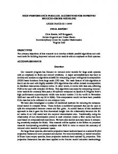
2.2.1 Eigensolvers A review of many eigensolvers was performed by Sunderland and Breitmoser [40] . The review found that the routines in ScaLAPACK performed the best in most circumstances. The only exception is if PESSL is installed on an IBM system, as this had similar routines to those of ScaLAPACK, but highly optimised for the specific architecture. A second technical report was published a year later by the same authors [41] comparing two routines from PLAPACK and two from ScaLAPACK for the solution of the symmetric eigenvalue problem. The study provided insight into how ScaLAPACK performs against another well established library. Fig-

17

ure 2.1 shows the execution time for the four algorithms (QR and MR3 from PLAPACK, and QR and D&C from ScaLAPACK). It can be seen that the D&C algorithm from ScaLAPACK is the fastest for all numbers of processors tested. Further results displayed in the report show that this was also the case for all matrix sizes investigated.

Figure 2.1: Time taken for the four routines to complete on a matrix size of 12,354. Routines includes QR and MR3 from PLAPACK, and QR (PDSYEV) and D&C (PDSYEVD) from ScaLAPACK. Taken from Breitmoser and Sunderland (2004) [41] .

2.2.2 Singular Value Decomposition From the parallel libraries listed in Table 2.2, the three libraries that include routines to compute the SVD of a rectangular dense matrix are PESSL, ScaLAPACK and the NAG parallel library. However, the PESSL library is only available on IBM systems and the NAG library is not open source. Therefore the ScaLAPACK is the only library which fulfils all the desired criteria.

2.3 Summary of Library Routines For libraries to be utilised in this project, they had to initially satisfy three conditions: they must be parallel, portable and available within the public domain. Several libraries satisfied two out of the three conditions; however, only the ScaLAPACK library fulfils all the desired requirements. Therefore routines from the ScaLAPACK library will be used for to implement the SVD and KLD methods.

18

Chapter 3

Test Cases and Numerical Implementations The following sections give details on the data sets that were used throughout the project and utilisation of the library routines. The final sections provide information on the structure of the code used for POD computations and the architectures that were used for testing.

3.1 Data Sets A range of cases of progressively higher complexity and size were used and are summerised in Table 3.1. This was necessary since the development of ideas and methods had to be assessed using serial code before developing the parallel methods. The lowest complexity flow tested was two-dimensional laminar flow over a circular cylinder and was used to gain initial results and verify the parallel library calls. Case No. 1 2 3 4 5

Test Case 2D Cylinder 2D Cylinder 2D Cavity 2D Cavity 3D Cavity

Flow Type Laminar Laminar Laminar Turbulent Turbulent

Grid Points 9,600 50,754 96,000 104,000 4,000,000

Reynolds Number 0.2 × 103 0.2 × 103 4.0 × 103 1.0 × 106 1.0 × 106

Mach Number 0.3 0.3 0.6 0.85 0.85

Table 3.1: Details of the test cases that will be used throughout the project.

19

3.1.1 Flow over a circular cylinder The flow over a circular cylinder is very distinctive and so it is a useful test case. It has also been studied using POD and so results from computations can easily be verified against published data.

[23, 24]

At Reynolds numbers between 4 and 40, the flow separates from the back of the cylinder and produces two stable counter-rotating vortices. If the Reynolds number is increased further, the vortices become unstable and begin to shed from the rear of the cylinder. The effect is known as the Karman vortex street. Figure 3.1 presents a visualisation of the vortex street using ink die in a water tunnel. It can be seen that the flow is highly periodic, with each vortex being shed alternately downstream in a regular fashion.

Figure 3.1: Circular cylinder wake at Reynolds number of 120, with a computational flow field inset for comparison.

Two 2D grids were constructed to compute the flow, one containing 9,600 points and the other 50,754 points. The computations were run at a Reynolds number of 200 (laminar flow) and a Mach number of 0.3. A total of 1000 timesteps were computed, with a flow field file being produced at every timestep. Approximately 100 timesteps were equal to one full oscillation cycle of the flow. Figure 3.1 also shows an instantaneous flow field with contours of vorticity, which was produced by a CFD computation on the smaller grid size. In a velocity field the vorticity, ξ , is defined as being

20

equal to the curl of the velocity [42] :

ξ = ∇ ×V

(3.1)

The vorticity is equal to twice the angular velocity in the flow and so by visualising this parameter, vortices in the flow can be seen. As with the experimental visualisation, the results from CFD computation shows the flow is asymmetric and vortices shed from the cylinder can be seen downstream. However, if the flow field was averaged over a large period of time (i.e. at least one flow oscillation cycle), then the result shows two symmetric vortices (Figure 3.2).

Figure 3.2: Averaged vorticity contours.

3.1.2 Cavity Flow At certain flow conditions, the flow over a cavity might be aperiodic and can contain various flow structures. As with the cylinder, a two-dimensional laminar test case was first computed. The grid is larger than both cylinder grids discussed in §3.1.1 and contained 96,000 points. Figure 3.3 presents the instantaneous flow-fields at four timesteps during the computation and represents one oscillation cycle of the flow. It can be seen that a vortex is created at the front of the cavity and grows as time progresses. Eventually it is shed at the rear of the cavity and a new vortex is generated at the cavity front. A grid of similar size that was suitable for the analysis of the two-dimensional turbulent cavity flow was also generated. The main grid for the cavity test case is three-dimensional and contains 4 million grid points. Due to the complexity of the flow and the high quantity of storage required, the case was only run for 80,000 time steps and 80 flow-field files are available. The 3D turbulent flow is more complex than the 2D flow and contains many more smaller and higher frequency structures.

21

(a) Timestep 500

(b) Timestep 510

(c) Timestep 520

(d) Timestep 530

Figure 3.3: Instantaneous flow fields of the two-dimensional laminar cavity flow.

22

3.2 Data Distribution When using the ScaLAPACK library, data contained in the input matrices was required to be ordered in a very specific way. This makes the computations on dense matrices as efficient as possible for distributed memory machines. The data layout that ScaLAPACK uses is based on the most efficient layout for Gaussian elimination (Figure 3.4). A two-dimensional block-cyclic distribution ensures that the processors will be load balanced throughout the computation. Figure 3.5 shows a two-dimensional cyclic distribution of processors. Each processor would have an n × n block of data, which then creates the 2D block cyclic data distribution.

Figure 3.4: Schematic showing Gaussian Elimination.

Figure 3.5: Schematic showing a two-dimensional cyclic distribution of processors.

23

3.3 Code Design The structure and information relating to the driver code for the SVD and KLD calculations will be explained here. The code was written in the C programming language and it can be seen in full in Appendix A. The code is is split into four different parts: the control program, data input and distribution, SVD or KLD calculation and output.

3.3.1 The Control Program The main program first reads the arguments given in the command line. These include the location of the files on disk and the start and end points of the calculation. Further details of how to run the code can be found in Appendix A. The main program then initialises MPI and sets up the process grid. The dimensions of the process grid are obtained using the MPI library, but it is then set up using the BLACS (Basic Linear Algebra Communication Subprograms) library. The ScaLAPACK library is written on top of four other libraries (Figure 3.6): BLAS (Basic Linear Algebra Subprograms), BLACS, LAPACK and PBLAS (Parallel BLAS). Therefore any routines in these four libraries can also be used in conjunction with ScaLAPACK. The call to the BLACS library produces a handle variable for the setup of the grid, which is then passed to any ScaLAPACK routines used in the code. The program then calls the data input subroutine,

ScaLAPACK PBLAS

BLACS

LAPACK

BLAS

Global Local

Message Passing Primitives (MPI, PVM, etc)

Figure 3.6: Schematic showing the ScaLAPACK software hierarchy.

24

the SVD or KLD subroutine (depending on which the user has specified) and the output subroutine.

3.3.2 Input and Output The input and output (I/O) was originally done using master I/O. Therefore all the data was read using the master processor and then distributed to all the other processors using a global broadcast command. After the SVD/KLD computations, all the results were collected on the master processor using a global reduction command and then written to disk. This method is only suitable for small problems where all the data can fit into the memory of a single processor. Therefore both the input and output needed to be made parallel. The most obvious solution would be to use MPI I/O; however, the flow-field files are stored in a format readable by visualisation software and so text information about the grid is also included throughout the file. Therefore, MPI I/O was not used in the program. The current version of the code outputs the data from each processor to file, then a single processor reads these files and outputs it in the right order. The U matrix is written in the same format as the flowfield files from the solver and so can be read by visualisation software. The S and V matrices are written as simple data files. Reading data from the flow-field files in parallel was more difficult, especially since it needs to be distributed on the processors in the correct format for the library calls (as discussed in §3.2). The parallel input is performed in two stages, with both stages using counters in order to ensure each processor reads the right data files. The first stage ensures each column of the process grid reads the data files in a block-cyclic fashion and the second stage then ensures that each processor reads the data in each file in a block-cyclic distribution.

3.3.3 SVD or KLD Calculation The calculation for the SVD and KLD are spread over four subroutines (two for each). The first subroutine for each method sets up the necessary arrays and performs any preliminary computational work. For the KLD method, this would involve a call to the PBLAS routine PDGEMM (Parallel, Double precision, General Matrix Multiplication) to calculate the covariance matrix.

25

The second subroutine is then called by the first and the parallel calculation of the SVD or KLD is performed. SVD and eigensolver algorithms were chosen from the ScaLAPACK library and are discussed in the following section. The full list of arguments for both routines can be found in Appendix B.

SVD The driver routine PxGESVD performs the SVD of a real M × N matrix in single or double precision and calls the recommended sequence of ScaLAPACK routines. It requires a distributed input matrix, A, and outputs distributed U and V matrices. The array containing the singular values is identical on all processors. It also requires an additional input array which allows space for the SVD routine to perform calculations.

Eigensolver (KLD) The driver routine PxSYEV computes the eigenvalues and the eigenvectors of a real symmetric N × N matrix in single or double precision by calling the recommended sequence of ScaLAPACK routines. The routine requires a distributed input matrix and outputs a distributed matrix containing the eigenvectors. The output array containing the eigenvalues is identical on all processors. As with the SVD routine, an additional input array is needed for workspace.

Passing Variables It is worth noting that since the libraries are written in Fortran 77, all variables have to be passed by reference when calling any of the routines. When the libraries are linked to a C program, passing single variables is a simple process. However, it means that when passing data in multi-dimensional arrays, all the data has to be contiguous in memory. This is not usually the case when allocating memory for multi-dimensional arrays in C. In the code shown in Appendix A, ensuring the data in multi-dimensional arrays was contiguous in memory was achieved by using the arralloc program provided by EPCC.

26

3.4 Architectures The dissertation will focus on two different architectures: HPCx and the Liverpool Beowulf cluster. The two architectures were chosen since they represent types of machines that many engineering problems are performed on. HPCx is the UK national supercomputing service and due to the large scale of the system, it would be very expensive to purchase and the running costs are high. Therefore this represents the type of system that a user would ’buy’ time on and use ’on demand’. The Beowulf cluster is more representative of a system that a user might own as it is relatively inexpensive to purchase and the running costs are low. A brief description of each architecture is given in the following section.

3.4.1 HPCx HPCx is a cluster of 160 IBM eServer 575 Power5 Symmetric Multi-processor (SMP) frames [43] . The eServer frames utilise the IBM Power5 processor, which is a 64-bit RISC processor with a clock rate of 1.5 GHz. There are two floating point multiply-add units, each of which can deliver one result per clock cycle, giving a theoretical peak performance of 6.0 Gflops per processor. The eServer frames contain 8 chips, which each chip containing two processors. Each processor has its own level 1 (L1) cache and a shared level 2 (L2) and level 3 (L3) cache. The L1 cache is split into a 32 Kbyte data cache and a 64 Kbyte instruction cache. The L2 cache is a 1.9 Mbyte combined data and instruction cache. The L3 cache is 36 Mbytes in size. Each frame has 32Gbytes of main memory, allowing 2Gbytes per processor [43] . The system’s 160 frames are connected through IBM’s High Performance Switch (HPS), also known as "Federation". Each eServer frame has two network adapters, with two links per adapter, giving a total of four links between each frame and the switch network [43] . The 2560 processors have a theoretical peak performance of 15 Tflops and on LINPACK [25] the system has achieved a peak performance of 12 Tflops[26] . The sustained performance of the system is approximately 6 Tflops.

27

3.4.2 Beowulf Cluster The second architecture is the Liverpool Beowulf cluster. The cluster consists of 130 Intel Pentium 4 processors, which have a clock speed of 2.8 GHz. The processor has two Arithmetic Logic Unit (ALU) for integer and logic arithmetic and one floating point (FP) multiply-add unit, each of which can output 2 single-precision operations or 1 double-precision operation per clock cycle [44] . This gives the Pentium 4 processor a theoretical peak performance of 11.2 Gflops in single precision and 5.6 Gflops in double precision. The processor has a 16 Kbyte L1 data cache, 1 Mbyte L2 combined data and instruction cache and 1 Gbyte of main memory. The processors are connected through a 100 Mbit switch. The performance of this switch would be much lower than the one installed in HPCx. Therefore computations involving high levels of communications would not complete as fast on this system as they would on HPCx. The 130 processors have a theoretical peak performance of 728 Gflops in double precision.

3.5 Summary The project used five different test cases with increasing grid size or flow complexity: two based on the laminar flow over a cylinder, one based on the laminar flow over a cavity and two based on turbulent flow over a cavity. The library routines were taken from the ScaLAPACK library, which needed a twodimensional block-cyclic distribution for mapping the data to the processors. The code reads the data from disk in parallel so the required mapping is created. The SVD or the KLD is then performed and the output from each processor is then written to disk. The project focused on two different architectures: HPCx (a cluster of SMPs) and the Liverpool Beowulf Cluster. It was deemed the two architectures are examples of systems that are utilised for many engineering problems.

28

Chapter 4

Initial Investigations into POD

4.1 Results from Serial Algorithms Serial programs were developed before any parallel programs in order to gain some initial insight into the SVD and KLD algorithms. Serial versions of the ScaLAPACK routines identified in §3.3.3 exist in the LAPACK library and so were used here. Using these serial routines would not only give valid experience of programming with scientific libraries, but would also give a set of results to validate the correctness of the parallel routines.

4.1.1 SVD The SVD of the two-dimensional circular cylinder data was performed using three methods: the first was with MATLAB, the second was with a routine from Numerical Recipes (NR) [36] and the third was using LAPACK [35] . Many of the MATLAB routines stored in the math library, including the SVD routine, are based upon LAPACK algorithms. This makes the results from MATLAB reliable and therefore good for validation purposes. The numerical recipes SVD routine was available in either Fortran90 or C. As with the ScaLAPACK library, the LAPACK routines are written in Fortran 77. The three outputs were compared in order to ensure the LAPACK routine was being called correctly. It can be seen from Table 4.1 that the MATLAB and LAPACK results were identical, which was

29

MATLAB 9.28416e+01 8.94843e+01 1.28008e+01 1.13731e+01

Mode 1 Mode 2 Mode 3 Mode 4

NR 9.28415e+01 8.94843e+01 1.28008e+01 1.13731e+01

LAPACK 9.28416e+01 8.94843e+01 1.28008e+01 1.13731e+01

Table 4.1: First four singular values for each method tested.

expected since the MATLAB routines are taken from the LAPACK library. Even when the results were compared to those from Numerical Recipes, the magnitude of mode 1 only differed by the last significant figure. The magnitude of the three other modes were identical to those of MATLAB and LAPACK.

4.1.2 Eigensolver The same check that was performed for the SVD was then performed for the eigensolver routines. As with the SVD, the eigensolver routines in MATLAB are implementations of those in the LAPACK library. It can be seen in Table 4.2 that the LAPACK library was being called correctly since the eigenvalues were identical to those from MATLAB.

Mode 1 Mode 2 Mode 3 Mode 4

MATLAB 8.53422e+01 7.92817e+01 1.62239e+00 1.28067e+00

LAPACK 8.53422e+01 7.92817e+01 1.62239e+00 1.28067e+00

Table 4.2: First four eigenvalues for each method tested.

4.1.3 Performance of Serial Routines The serial programs developed using the LAPACK routines were tested to assess the relative performance. The programs were tested with the small cylinder grid (test case 1 in Table 3.1) using 400 snapshots. Table 4.3 compares the performance of the SVD library routine, the eigensolver library routine and the KLD method. The execution times for the whole SVD method are not shown as the times were almost identical to the times for the SVD library routine. It can be seen that the eigensolver routine executed substantially quicker than the SVD routine. However, since it operated on the covariance matrix (refer to §1.3.2), the matrix size was only 400 × 400, whereas the SVD library routine operated on the entire input data matrix, which had dimensions of 9600 × 400. Therefore a comparison between

30

the library routines is not a fair one. The two methods can be compared since the KLD method utilised the PBLAS routine DGEMM (Double precision, General Matrix Multiply) to perform a matrix-matrix multiply before and after the computation of the eigenvalues. Therefore the KLD method as a whole operated on the same size matrix as the SVD routine. Even with the extra calls and computations, the KLD method is over twice as fast as the SVD for this matrix size. It can also be seen in Table 4.3 that there is a large difference in the times that were gained on HPCx and on the Beowulf cluster. It is thought that the difference was likely due to the high level of optimisation used when the libraries were compiled and installed on HPCx.

4.2 Data Compression After the SVD or KLD has been calculated, the magnitude of the singular values or eigenvalues are equivalent to the energy of the flow captured by that mode (refer to §1.3.2). For the flow over a cylinder, the magnitude of each mode is plotted in Figure 4.1. It can be seen that the modes for both methods come in pairs. When this occurs, it suggests that there is symmetry within the flow. Also shown in Figure 4.1 is the cumulative energy for increasing amounts of modes. For both methods the first four modes capture over 95% of the energy of the flow. Increasing this to eight modes captures over 99% of the energy. The flow-field files were then reconstructed using four and eight SVD modes (Figure 4.2). The reconstructed files from KLD calculations are not shown as they were very similar to the SVD reconstructions. It can be seen that the reconstruction using four modes has good agreement with the original flow-field. The reconstruction using eight SVD modes is even better, only displaying very small discrepancies. Figures 4.2(d) and 4.2(e) are the normalised differences between the original flow-field data and the reconstructed data. Therefore at every point in the flow, the following computation is performed: Normalised Di f f erence = (XR − XO )/XO

Time on HPCx (s) Time on Cluster (s)

SVD 3.31 16.66

Eigensolver 0.23 0.49

(4.1) KLD 1.61 5.56

Table 4.3: Execution times of the serial programs on the small cylinder grid (test case 1).

31

Figure 4.1: The energy fraction for each mode and the cumulative energy for the flow over a cylinder.

where XO is the value of the data in the original data file and XR is the value of the data in the reconstructed data file. It can be seen from both figures the main vortical structures of the flow were not affected when only a small fraction of the modes were used. Only the space around the structures in the reconstructed flow-fields differ to those of the original flow-fields, with the difference being less than 1% at every point in the flow when using eight modes. The level of data compression that can be achieved by the two methods was investigated. Table 4.4 shows the storage requirements for the original flow field files and the SVD files for one flow oscillation. The results show that when using eight modes, the SVD files require over 12 times less storage space compared to the original flow field files. Also shown is the difference in storing the SVD calculated from 100 files and from 10 files in one flow oscillation. It can be seen that only the storage requirements of the right singular vector, V , change due to the increased number of files and so it is advantageous to use as many files as possible to calculate the SVD or KLD.

32

(a) Original at timestep 630

(b) Reconstruction using 4 modes

(c) Reconstruction using 8 modes

(d) Difference using 4 modes

(e) Difference using 8 modes

Figure 4.2: Original flow-field data compared to reconstruction using four and eight modes for the laminar flow over a cylinder.

All Files on Disk SVD, 10 Files SVD, 100 Files

U(Kbytes)

S(Kbytes)

V (Kbytes)

9830 9830

0.8 0.8

6.5 65

Total (Mbytes) 120 9.6 9.7

Table 4.4: Size of the original files on disk compared to the storage required for 8 SVD modes.

33

4.3 Verification of Parallel Library Call The output from the parallel routines can be compared to the output from the serial routines, since this is now known to be correct. Table 4.5 shows the singular values and eigenvalues produced by the parallel ScaLAPACK and serial LAPACK calls. It can be seen that they are identical and so it can be concluded that the parallel library calls are correct.

Mode 1 Mode 2 Mode 3 Mode 4

KLD LAPACK ScaLAPACK 8.53422e+01 8.53422e+01 7.92817e+01 7.92817e+01 1.62239e+00 1.62239e+00 1.28067e+00 1.28067e+00

SVD LAPACK ScaLAPACK 9.28416e+01 9.28416e+01 8.94843e+01 8.94843e+01 1.28008e+01 1.28008e+01 1.13731e+01 1.13731e+01

Table 4.5: First four eigenvalues for each method tested.

4.4 Summary Serial programs were developed before parallel programs in order to gain some initial insight into the SVD and KLD algorithms. The LAPACK versions of the parallel ScaLAPACK routines were utilised for the programs. It was shown that the KLD algorithm is not only a faster method, but also better in terms of data compression as it required less modes to reconstruct the flow. The serial results were then used to ensure the parallel programs gave the correct output.

34

Chapter 5

Parallel Performance for Small Problems To gain some insight into the performance of the parallel code, it was initially tested on the first two test cases from Table 3.1. The data from both these cases were from the laminar flow over a cylinder, with the medium data set being 5 times larger than the smallest data set in terms of grid points. Also the smallest data set used 400 files, while the medium data set used 1000 flow-field files. The results shown were performed on HPCx only. Unfortunately, there were difficulties in installing the ScaLAPACK library onto the cluster and so no results were acquired.

5.1 Distribution Blocksize The first parameter to be investigated was the blocksize for the two-dimensional block-cyclic distribution. The ScaLAPACK reference manual [29] suggests using a blocksize as large as possible although it is very dependent on the algorithm and the size of the data set being used. Both the SVD and the eigensolver routines were tested on 16 and 32 processors for the smallest data set (test case 1), the results of which can be seen in Figure 5.1 Many conclusions can be drawn from these initial results. Firstly, it can be seen that the eigen-

35

Figure 5.1: Execution time for the SVD and eigensolver routines for varying blocksize in the 2D blockcyclic data distribution. Results are for the small problem size (test case 1).

solver routine has a substantially quicker execution time than the SVD routine on both numbers of processors. However, the execution times for the eigensolver routine on 16 processors were faster than those on 32 processors, which indicated that the data set used was too small and so the computation was dominated by the communication between processors rather than the computation of the eigenvalues and eigenvectors. It can also be seen that the variation of performance curves for the SVD routines are much more pronounced than those of the eigensolver routines for increasing blocksize. For the SVD routine, the execution time on 16 and 32 processors was approximately 0.97 and 0.57 seconds respectively for a blocksize of 2. As the blocksize was increased, the execution time drops significantly and reached a minimum at a blocksize of 8, where the execution times were 0.74 and 0.47 seconds. The difference in times equates to a reduction of 24% and 18% in the execution times for 16 and 32 processors respectively. For the eigensolver routine, the curve was much flatter and reached a minimum at a blocksize of 16. Table 5.1 shows the minimum and maximum number of rows and columns across 16 processors for three different blocksizes. For a blocksize of 4, the amount of data on all the processors is the same

36

Rank Minimum Maximum % Imbalance

Blocksize: 4 Cols Rows 2400 100 2400 100 0 0

Blocksize: 8 Cols Rows 2400 96 2400 104 0 8.3

Blocksize: 32 Cols Rows 2400 96 2400 112 0 16.7

Table 5.1: Data distribution on 16 processors for 3 different blocksizes.

and so the processors are perfectly balanced. When the blocksize is increased to 8, there is an imbalance of 8 rows (19,200 data points) between the processors. Since the processors have different amounts of data, the amount of work that the processor would have to perform would also be different. Therefore it is likely that the imbalance of data would translate to a load imbalance. However, Figure 5.1 shows that the execution time for both routines decreases despite this imbalance and so in this case it can be concluded that the advantage of increasing the blocksize outweighed the performance deficit created by the load imbalance. The load imbalance increases further at a blocksize of 32, when it has a value of 16 rows (38,400 data points) between the processors. Figure 5.1 shows that when increasing the blocksize from 8 to 16, the execution time only increased for the SVD routine. Therefore it can be concluded that the SVD routine is more sensitive to the larger load imbalances than the eigensolver routines.

5.2 Matrix Sizes The effect of the number of snapshots (matrix dimension N) was investigated to see how the execution time of each routine varied with matrix size. Figure 5.2 gives the execution time for the computation of the SVD, KLD and the eigensolver library routine call on the small cylinder grid (test case 1). For the SVD, the only extra work needed outside calling the routine is setting up the array descriptors, whereas the KLD method has a matrix-matrix multiply before and after the library routine call. However, since the matrix operations are done in parallel on the distributed matrices, the method is still faster than the SVD library call. The trend continues for test case 2 (Figure 5.3), which is the larger problem size. It can be seen that with 1,000 snapshots in the matrix, the KLD method is almost 5 times quicker than SVD.

37

Figure 5.2: Execution times for increasing number of snapshots in the matrix. Execution times are for two POD methods and the eigensolver library routine call for test case 1.

Figure 5.3: Execution times for increasing number of snapshots in the matrix. Execution times are for two POD methods and the eigensolver library routine call for test case 2.

38

Figure 5.4: Execution times for increasing number of snapshots in the matrix comparing test cases 1 and 2 for both POD methods.

The data presented in Figures 5.2 and 5.3 were combined to give the execution times for total points in the matrix. Figure 5.4 shows that the execution times of both methods are more effected by the number of snapshots in the matrix than the number of spatial points. For a given number of total elements in the input matrix, both methods execute faster when the ratio between M and N is large. From this, it can be concluded that computing the SVD or KLD of a very large problem with only a few snapshots (which is the case with the three-dimensional cavity flow test case) is likely to take a relatively short amount of time.

5.3 Scaling Performance The scaling performance of both the library routines and the POD methods needed to be investigated. It would be desirable to have the routines scale well in terms of speed-up; however, it is more desirable to investigate which routine performs best in absolute terms. Therefore comparisons between the SVD and KLD methods are done with the execution times.

39

Figure 5.5: Execution times on increasing number of processors. Execution times are for two POD methods and the eigensolver library routine call for test case 1.

The execution times were recorded for test cases 1 and 2 on increasing amounts of processors. Figure 5.5 compares the performance of the library routines and the POD methods on test case 1. The execution time for the SVD decreases steadily between 2 and 8 processors, then looks to level off at 16 processors. However, there is then a decrease in execution time at 32 processors, which could be due to cache effects and will be further investigated in the following section. The execution times for the eigensolver library routine fluctuate, but stay at approximately 0.2 seconds for all numbers of processors tested. The fact that the execution time does not decrease with the increase in processors suggests that the input matrix is too small. Therefore the calculation is dominated by the communication between the processors rather than the computations that are performed on each processor. The KLD method shows a reduction in execution time with increasing numbers of processors. Therefore since the eigensolver does not benefit from the increase in numbers of processors, the routine that performs the matrix multiplications before and after the eigenvalue computation must benefit. A similar trend is seen for the scaling performance for test case 2 (Figure 5.6), although the execution times for both the SVD and KLD methods are an order of magnitude higher than for test case

40

Figure 5.6: Execution times on increasing number of processors. Execution times are for two POD methods and the eigensolver library routine call for test case 2.

1. The SVD routine has an execution time of almost 20 seconds on 16 processors, which decreases to 10 seconds on 32 processors. The execution time reduces further and on 512 processors, it is approximately 2 seconds. Therefore the routine scales well for low numbers of processors for this matrix size, but does not scale up to large numbers of processors. As with the smaller problem size, the execution times for the eigensolver routine fluctuate and actually increase slightly as the number of processors becomes very large. Therefore it can be concluded that the problem size is still too small for the number of processors being used.

5.4 Cache Effects The performance of the library routines are not only influenced by the amount of data in the matrix, but also by how quickly the processors can access that data. Figure 5.7 shows the boundaries for the cache levels on the Power5 processors and data distribution for test cases 1 and 2. It can be seen that for the smaller problem size the distributed data arrays can be stored in the L3 cache on 2 processors and in the

41

Figure 5.7: Data cache size on HPCx and data per processor for small and medium grid sizes.

L2 cache on 32 processors. For the larger problem size, the data can be stored in the L3 cache on 32 processors and in the L2 cache on 512 processors. Looking again at Figure 5.5, the slight increase in performance displayed between 16 and 32 processors for the SVD routine call could be due to the input data matrix being stored on the L2 cache instead of the L3 cache. However, the input data matrix is not the only input array to the library routine calls. As shown in §3.3.3, a double precision array is also needed as workspace. Therefore the size of the workspace and where it is stored could also affect the performance of the library routines.

5.4.1 Size of the Workspace Eigensolver Subroutine PDSYEV The routine PDSYEV is a driver routine for calculating eigenvalues and eigenvectors. Although only a single call is performed by the main program, the library actually calls a predetermined sequence of subroutines. Therefore the workspace required for all the subroutines needs to be allocated before the driver routine is called. The PDSYEV makes two main calls to perform the following operations:

42

1. Reduce the symmetric N × N matrix to a symmetric tridiagonal matrix. 2. Calculates the Eigenvalues and Eigenvectors of the symmetric tridiagonal matrix using the QR algorithm. The formulation for the size of the workspace is given as: Size o f workspace >= (5 × N) + (N × LDC) + MAX(SizeMQRLe f t, QRmem) + 1

(5.1)

where N is the dimension of the global matrix, (N × LDC) is equal to the amount of data on each processor from the input matrix, SizeMQRLe f t and QRmem are array sizes which relate to calculating the eigenvalues and eigenvectors using the QR algorithm. QRmem is dependent on the global matrix dimensions whereas SizeMQRLe f t is mainly dependent on the blocksize and data distribution. The third terms in the equation above are small, therefore as the number of processors increases, the first term becomes dominant since this is independent of the number of processors used. Overall, the amount of space required for the workspace in this routine is small compared to the size of the data matrix.

SVD Subroutine PDGESVD As with the eigensolver routine, the SVD routine PDGESVD is a driver and makes two main calls to perform the following operations: 1. Reduce the general M × N matrix to a bidiagonal matrix. 2. Calculates the SVD of the bidiagonal matrix. The formulation for the size of the workspace is given as: Size o f workspace >= 2 + (6 × MAX(M, N)) + MAX(Watobd,Wbdtosvd)

(5.2)

where M and N are the dimensions of the global matrix, Watobd is the workspace size needed to transform the general matrix to a bidiagonal matrix and Wbdtosvd is the workspace size needed to calculate the SVD from the bidiagonal matrix. The calculations for both Watobd and W bdtosvd are quite long and depend on many different parameters. The main dependencies though are the blocksize and the data distribution, which are local to each processor. The second term in the formulation is based on the global matrix size and so stays constant irrespective of the amount of processors used in the computation. Since

43

Figure 5.8: Data cache size on HPCx and size of input arrays (data matrix and required workspace) for the SVD subroutine. The curves are for small and medium cylinder problems (test cases 1 and 2).

the second term reduces in size as the number of processors increases, the third term becomes more dominant as the number of processors increases. The size of the workspace was recorded for increasing numbers of processors. This was then added to the size of the data matrix and plotted in Figure 5.8. It can be seen that for both problem sizes the total size of the input arrays would fit into the L3 cache on most numbers of processors tested. Therefore it is more difficult to account for the increase in performance described previously in §5.3. The only way to be certain about how the data is stored and the effect that the cache has is to use performance analysis programs. Through these, hardware counters that look at aspects such as cache hits and misses can be analysed. However, this was not done for the present study for two reasons: the first is that for large programs, this becomes complicated and the analysis of the output is a lengthy and difficult process. The second is that the aim is to use the parallel code to compute the SVD or KLD for very large problems. Therefore the data would not fit into the cache of the system and so the ratio of cache misses to hits would probably be very high.

44

5.5 Summary An initial insight into the performance of the SVD and KLD methods was gained. It was shown that the eigensolver routine had a substantially quicker execution time than the SVD routine on all numbers of processors. However, looking at the execution times for the eigensolver routine revealed that the data set used was too small and so the computation was dominated by the communication between processors rather than the computation of the eigenvalues and eigenvectors. An attempt was made to justify the performance variation of the methods by looking at the data and cache sizes. However, this was inconclusive and would not apply for large scale problems.

45

Chapter 6

2D and 3D Cavity Results

6.1 2D Laminar Flow The first cavity case to be computed was the laminar flow over a cavity. The laminar flow has much less complexity than the turbulent flow due to the lower Reynolds number that the simulation was performed at. The magnitudes of the SVD and KLD modes are shown in Figure 6.1 and it can be seen that like the laminar flow over a cylinder, a significant amount of the energy of the flow is contained in relatively few modes. For both methods, over 95% of the original flow can be reconstructed using just 10 modes. If that is increased to 20, then 99% of the original flow-field can be reconstructed. To visualise what the modes of the flow look like, the first four modes are shown in Figure 6.2. These four modes represent 75% of the energy of the flow and in the caption in each figure, the individual contribution is shown. Figure 6.3 shows the reconstructed flow-field at one timestep that is gained when using just these modes. Figure 6.3(c) shows that the difference between the original flow-field and the reconstructed flow-field is less than 10% at all points in the flow and the areas that are most affected are at the front of the cavity. Comparisons between the original flow-fields and reconstructions at one timestep using 10 and 20 modes are shown in Figure 6.4. It can be seen that both reconstructed flow-fields are very similar to the original. The normalised differences (Figures 6.4(d) and 6.4(e)) show that the areas around the front

46

Relative Cumulative Energy (%)

100 80 60 40 20 0 0

SVD POD 10

20 30 Number of Modes

40

Figure 6.1: The energy fraction for each mode and the cumulative energy for laminar cavity flow.

of the cavity still had the highest variation from the original flow. Although, when using 20 modes, the variation is less than 1% at all points in the flow. This result is in agreement with the analysis of the eigenvalues (Figure 6.1).

6.2 3D Turbulent Flow 6.2.1 Probe Files An initial investigation into the three-dimensional cavity was done using the output from probes in the flow. When a computation is started using the CFD solver, the user can specify coordinates of points in the flow where detailed information is required. Information about the flow is recorded at every computational timestep and stored in ’probe files’ in ASCII format. For the three-dimensional cavity case, 250 probes were specified in the cavity and so this forms a very course grid over which an analysis with high temporal resolution can be performed. Figures 6.5, 6.6 and 6.7 show reconstructions of the time signals using 10, 50 and 100 modes respectively. Also shown in the figures are the frequency spectra, which give a clear picture of the effect of increasing the number of modes when trying to reconstruct the original signal. It can be seen that using just 10 modes to reconstruct the data almost captures the time signal. The magnitude of the

47

(a) Mode 1 (32% of the flow)

(b) Mode 2 (20% of the flow)

(c) Mode 3 (13% of the flow)

(d) Mode 4 (10% of the flow)

Figure 6.2: Modes 1 to 4 for the two-dimensional laminar cavity. The SVD was performed on the pressure fluctuations inside the cavity.

48

(a) Original at timestep 900

(b) Reconstruction using 4 modes

(c) Difference using 4 modes

Figure 6.3: Original flow-field data compared to reconstruction using 4 modes for laminar flow over a two-dimensional cavity.

49

(a) Original at timestep 900

(b) Reconstruction using 10 modes

(c) Reconstruction using 20 modes

(d) Difference using 10 modes

(e) Difference using 20 modes

Figure 6.4: Original flow-field data compared to reconstruction using 10 and 20 modes for laminar flow over a two-dimensional cavity.

50

pressure fluctuations are smaller then the original time signal but the main outline is represented. The frequency spectrum shows that the reconstruction is only similar to the original data below a frequency of 1 kHz. Recall that in §1.3.1 it was stated that it might be satisfactory to reconstruct the time signal accurately for only the lower frequencies as long as the high intensity tones are reconstructed well. From this result, it might be the case that storing as few as 10 modes might be sufficient for even the turbulent cavity flow case. When the number of modes used for the reconstruction was increased to 50, the pressure signal was captured with more accuracy. Looking at the time signal, the amplitudes of the peaks are better represented and more of the detail is captured. This is also reflected in the frequency spectra, where the reconstructed data is very close to the original data for the lower frequency peaks. The curve for the reconstructed data is also much closer to the original data for the higher frequencies. The reconstruction using 100 modes has very few discrepancies when compared to the original data. The time signal for both curves are almost identical and there is only a very small difference in the frequency spectra in the high frequency parts. In conclusion, it can be seen that the low frequency part of the signal can be represented with relatively few modes. The peaks in the low frequency end of the spectrum are caused by the large structures in the flow and so these can be captured with a small amount of modes. Above a frequency of about 1 kHz, the signal is mostly due to noise and so representing this part of the signal is not as important.

6.2.2 Flow-Field Data The SVD and KLD for the three-dimensional cavity flow-fields were computed. The magnitude of the SVD and KLD modes are shown in Figure 6.8. It can be seen that the initial modes do not contain as much of the flow energy as with the laminar flow over the cavity. Therefore many more modes might be needed for an accurate reconstruction of the flow. From the reconstructions of the flow over a cylinder, it was assumed to be the case that at least 90% of the flow would be needed for an accurate representation. However, it was seen from the probe files in §6.2.1 that when the flow was decomposed using 250 modes, only the first 50 needed to be stored for a good reconstruction of the signal.

51

(a) Time signal.

5

10

Original Signal Reconstruction

PSD of Pressure (Pa2/Hz)

4

10

3

10

2

10

1

10

0

10

0

500

1000

1500

2000

Frequency (Hz) (b) Frequency spectrum.

Figure 6.5: Reconstruction of pressure signal using 10 modes.

52

2500

3000

(a) Time signal.

5

10

Original Signal Reconstruction

PSD of Pressure (Pa2/Hz)

4

10

3

10

2

10

1

10

0

10

0

500

1000

1500

2000

Frequency (Hz) (b) Frequency spectrum.

Figure 6.6: Reconstruction of pressure signal using 50 modes.

53

2500

3000

(a) Time signal.

5

PSD of Pressure (Pa2/Hz)

10

Original Signal Reconstruction

4

10

3

10

2

10

1

10

0

500

1000

1500

2000

Frequency (Hz) (b) Frequency spectrum.

Figure 6.7: Reconstruction of pressure signal using 100 modes.

54

2500

3000

Figure 6.8: The energy fraction for each mode and the cumulative energy for the cavity flow.

The execution times for both the methods are shown in Figure 6.9. It can be seen that the execution times for the eigensolver routine actually increased with the number of processors used in the computation. Since there were only a small number of flow files, the covariance matrix was very small. Therefore when large numbers of processors were used, the execution times were higher due to the increased amount of communications that were needed between the processors. As with the small problems discussed in Chapter 5, the KLD method was substantially quicker than the SVD method for all numbers of processors tested and the shapes of the curves were similar. However, at present, it is unclear why the curves of both programs follow the same profile. Figure 6.10 displays iso-surfaces of pressure for the averaged flow-field. It can be seen that even though the geometry of the cavity is symmetrical about the centerline of the cavity, the averaged flow is not quite symmetrical. Iso-surfaces of pressure for modes 1 to 3 from the SVD calculation are given in Figure 6.11. Since the averaged flow is not symmetrical, the modes are also not symmetrical. The 3D cavity was then reconstructed using 10 and 20 modes. Figure 6.12 shows the original flow-field at one time instant and a reconstruction using 10 modes. For clarity, slices down the centerline

55

Figure 6.9: Execution times on increasing number of processors. Execution times are for two POD methods and the eigensolver library routine call for test case 5.

Figure 6.10: Iso-surfaces of averaged pressure for 3D cavity.

56

(a) Mode 1

(b) Mode 2

(c) Mode 3

Figure 6.11: Iso-surfaces of pressure for 3D cavity. Modes 1 to 3 are shown.

57

(a) Original at timestep 4500

(b) Reconstruction using 10 modes

(c) Difference using 10 modes

Figure 6.12: Original flow-field data compared to reconstruction using 10 modes for turbulent flow over a 3D cavity.

58

(a) Original at timestep 4500

(b) Reconstruction using 20 modes

(c) Difference using 20 modes

Figure 6.13: Original flow-field data compared to reconstruction using 20 modes for turbulent flow over a 3D cavity.

59

of the cavity are shown. It can be seen that the two flow-fields look similar, although the reconstruction lacked some of the small scale detail of the original. Figure 6.12(c) highlights the extent that the two flow-fields differ and the locations that were most affected. It shows that areas close to the shear layer towards the rear of the cavity were most affected. However, even though only a small number of modes were used, the difference between the original and the reconstruction was a maximum of approximately 5% anywhere in the flow. When the number of modes was increased to 20 (Figure 6.13), the reconstruction improved slightly, although it still lacked the small scale detail of the original. Figure 6.13(c) shows that the differences between the two are much less than when using only 10 modes. However, the maximum difference is still approximately 5% at any point in the flow.

6.2.3 Data Compression For a problem of this size, the size of the matrix containing the spatial modes (U) was much larger than the matrix containing the time variant part (V ) or the eigenvalues/singular values (S). This was also shown in 4.4 for the small matrix size. Since the U matrix was written out in the same format as the flow-field files (§3.3.2), each mode that is produced from performing the SVD or KLD is the same size on disk as one of the flow field files (i.e. storing 20 modes on disk will required the same amount of space on disk as storing 20 flow-field files). Therefore both the methods have the potential to substantially reduce the amount of data stored for even complex flows.

6.3 Summary It was shown that, as with the laminar flow over a cylinder, the laminar flow over a cavity could be reconstructed to a high level using very few modes. From an initial analysis of the eigenvalues for the 3D turbulent flow over a cavity, it was assumed that the number of modes that would have to be stored would be very high. However, from an analysis of the probes, it was found that the low frequency end of the spectrum could be reconstructed using just 10 modes. Reconstructing the flow-fields from 10 modes showed that only the basic flow structures were reconstructed.

60

Chapter 7

Compatibility with the CFD Solver The usage of SVD and KLD computations with a CFD solver is discussed in this chapter. Firstly, using the parallel code for post processing is summarised, then two candidate methods for full integration are discussed.

7.1 Post-Processing of the Results The simplest method of implementation is to compute a set of solutions in time, then perform the SVD/KLD on the complete data set to gain the modes of the solution. The results above and from Chapters 4, 5 and 6 were gained using this method. Unfortunately the method is restricted by disk space required to store all the time solution files and by the amount of memory on the target architecture. Another constraint would be the input and output (I/O) of the data from disk to the processors, as reading large amounts of data from file takes large amounts of time. These issues are reflected in the work mentioned in Refs [22–24, 45] , as the size of the problems are small in comparison to the 3D cavity flow in terms of both grid size and flow complexity. The SVD and KLD for the full three-dimensional cavity flow problem reported above were gained on HPCx. To gauge what is possible using such an architecture (where it has large amounts of memory per processor), the maximum value of N (i.e. number of snapshots) for the grid size needed to be found. A modification to the code allowed data to be copied and added to the data matrix and so minimal

61

Figure 7.1: Execution times for increasing number of snapshots in the matrix. Execution times are for two POD methods and the eigensolver library routine call on the large grid size.

time could be spent reading data from disk. After numerous test runs, the maximum was found to be approximately 2,240 when using 256 processors (Figure 7.1). Even though the computation is possible, in practice it is not a viable method since it would take a very large amount of time to read from the disk when compared to the time taken to perform the computation. As stated in chapter 1, each one of the flow field files is 450 Mbytes in size and so to read the data in the memory from file would take a large amount of time. Therefore the computation of the SVD or KLD needs to be done immediately after the solver has computed the solution for the time step. This would require a method for integrating the calculation of the POD with the solver and also an incremental method for calculating the POD.

7.2 Integration with the CFD Solver 7.2.1 Method 1 Most modern architectures are based on the MIMD (Multiple Instruction, Multiple Data) architecture [46]

and so each processor does not have to execute the same set of instructions. The first method for

62

integration could use a small subset of the available processors to calculate the POD and so the rest would be used for the computation of the solution files. When the flow field information became available on the processors, they would send the data to the appropriate processor as defined by the two-dimensional block cyclic distribution. After all the data had been received, the calculation of the POD or SVD would be performed and the output written to disk. Although the method would work, it would involve a large amount of communication to transfer the data from the main set of processors to the small subset of processors.

7.2.2 Method 2 The most desirable method for implementation would be to calculate the POD using the same processors that are computing the CFD solution. The schematic in Figure 7.2 shows the process that would be performed, starting from distributing the multi-block grid onto the available processors. During the calculation, the solver produces output from each timestep, which gets added to the data matrix. Since each processor computes solutions for the same section of the grid at every timestep, the data stored on the processors looks like a one-dimensional block-cyclic distribution, not like the two-dimensional blockcyclic distribution that ScaLAPACK requests. However, even though the documentation for the library routines states that the decomposition should be two-dimensional, a one-dimensional block-cyclic data distribution still produces the correct output. The next stage was to assess the degradation in performance of the library routines due to the change in data distribution.

7.3 Results for 1D Block-Cyclic Distribution Figures 7.3 and 7.4 compare the performance of the library routines and the POD methods for a 2D and 1D data distributions. From Figure 7.3 it can be seen that the SVD routine is largely unaffected by the change in data distribution. The same cannot be said for the eigensolver routine, where there is a large performance degradation as the number of processors used in the calculation increased. Comparing the performance of the SVD and KLD methods, it can be seen that for low numbers of processors, the KLD is still the faster method. However, due to the decrease in performance of the

63

Figure 7.2: Schematic showing the output of the solver and how the data would be arranged in a 1D block-cyclic distribution.

Figure 7.3: Execution times on increasing number of processors. Execution times are for the library routines on 2D and 1D block-cyclic distributions.

64

Figure 7.4: Execution times on increasing number of processors. Execution times are for the two POD methods on 2D and 1D block-cyclic distributions.

eigensolver routine in the KLD method, the performance of the SVD matched that of the KLD for larger numbers of processors. The call to the matrix-matrix multiply routine PDGEMM makes up the extra computational time in the KLD method. Therefore the change in performance of the routine with the change in data decomposition was checked. Figure 7.5 shows the speed-up curves for the PDGEMM routine for both decompositions. It can be seen that both decompositions scale almost linearly and that the change has very little effect on the performance. There is only a small decrease for the largest number of processors tested.

7.4 Incremental Methods As stated in §7.2.2, for full integration into the solver, the same processors that perform the CFD calculation should also perform the POD computation. Therefore an incremental method of calculating the SVD or POD was needed. The method for calculating the SVD incrementally was based on the method by

65

Figure 7.5: Speed-up curve for the matrix-matrix multiply routine PDGEMM in PBLAS. Curves are for 1D and 2D block-cyclic data distributions.

Brand [47] . However, no method for the calculating KLD was found and so only an incremental method for the SVD was implemented. The incremental SVD method is as follows: the SVD of an initial data matrix is calculated as before, providing the initial U, S and V matrices. These can be updated with either one new column of data or a matrix containing multiple new columns of data. The first step was to implement a version of the algorithm in serial. The routine uses the LAPACK SVD routine to perform the updating of the three matrices. Figure 7.6 shows the initial results from the updating of the SVD of the small cylinder data set (case 1). At present, there is one small issue with the updating of the SVD. If the SVD matrices are only updated a small number of times, the output is the same as performing one computation of the SVD on the whole data matrix. The incremental SVD curve in Figure 7.6 was updated after adding every new column of data. The most significant singular values remain unchanged after the updating; however, at approximately the 30th singular value, the values differ from those of the original SVD. It is thought that this could be due to a loss of orthogonality of the U and V matrices through numerical error [47] . It must also be stressed that even though the decomposition is

66

5

Magnitude of Singular Value

10

Incremental SVD SVD

0

10

−5

10

0

20 40 60 80 Number of Snapshots in Matrix

100

Figure 7.6: Comparison of the singular values produced by the traditional post-processing SVD and the incremental SVD routine.

67

slightly different through using the incremental SVD, if all the modes are used for a reconstruction, then the original data matrix is recreated and no information about the data is lost.

7.5 Summary For the largest data set (test case 5), the maximum number of files that could be processed was determined to be 2,240. Afterwhich, the system does not have enough memory to store the input data and carry out the SVD or KLD calculations. However, reading in 2,240 files from disk would take a large amount of time. Therefore the calculations need to be carried out directly after the simulation. The incremental SVD was investigated so that the SVD decomposition could be updated when new data became available. If the SVD matrices were only updated a small number of times, the output was the same as performing one computation of the SVD on the whole data matrix. However, if a large number of updates were performed, the singular values start to differ. It is thought that this could be due to a loss of orthogonality of the U and V matrices through numerical error.

68

Chapter 8

Conclusions and Future Work The main objective of the project was to assess the SVD and KLD methods as data compression techniques. A significant part of both methods was done using routines from scientific libraries. Since this project was based on the CFD solver at the University of Liverpool, any libraries utilised had to conform to three criteria: they must be parallel, portable and be available within the public domain. Several libraries satisfied two out of the three conditions; however, only the ScaLAPACK library fulfilled all the desired requirements. Therefore routines from the ScaLAPACK library were used for to implement the SVD and KLD methods. The project used 5 different test cases with increasing problem size or flow complexity. An initial insight into the parallel performance of the SVD and KLD methods was gained using the small problems. Test cases 1 and 2 were tested on up to 64 and 512 processors respectively. It was shown that the eigensolver routine had a substantially quicker execution time than the SVD routine on all numbers of processors for both test cases. However, looking at the execution times for the eigensolver routine revealed that the data set used was too small and so the computation was dominated by the communication between processors rather than the computation of the eigenvalues and eigenvectors. The largest test case was also tested up to 512 processors and since there were only a small number of flow files, the result was the same as the results from the smaller test cases. Analysis of the ’probe’ files (which are high in temporal resolution but low in spatial resolution)

69

from the turbulent flow over a cavity show that only a limited number of modes are needed to recreate the desired data. Both the SVD and KLD methods were tested using 250 spatial coordinates and from this, only 50 modes needed to be stored. From the flow-field files (which are high in spatial resolution but relatively low in temporal resolution when compared to the probe files) it was shown that if 50 files were used to calculate the SVD or KLD, then only 20 needed to be stored in order to recreate the flow to within 5% at each spatial point. Each mode that is produced from performing the SVD or KLD is the same size on disk as one of the flow field files. Therefore both the methods have the potential to substantially reduce the amount of data stored, even for complex flows. The performance of the library routines for 2D and 1D data distributions were compared as a 1D distribution would be required if the method was integrated into the Liverpool solver. The SVD routine was largely unaffected by the change in data distribution, whereas the eigensolver routine suffered a large performance degradation as the number of processors used in the calculation increased. Comparing the performance of the SVD and KLD methods, for low numbers of processors the KLD method was still the faster method. However, due to the decrease in performance of the eigensolver routine in the KLD method, the performance of the SVD method matched that of the KLD method for larger numbers of processors. The incremental SVD was investigated so that the decomposition could be updated if new data became available. If the SVD matrices are only updated a small number of times, the output is the same as performing one computation of the SVD on the whole data matrix . However, if a large number of updates were performed, the singular values start to differ. It is thought that this could be due to a loss of orthogonality of the U and V matrices through numerical error. It must also be stressed that even though the decomposition is slightly different through using the incremental SVD, if all the modes are used for a reconstruction, then the original data matrix is recreated and no information about the data is lost. Further investigation into the incremental SVD needs to be performed to see if the problem can be solved. Also, since the KLD method was shown to be the faster and more optimal method, investigations into incremental KLD should be performed.

70

Bibliography [1] Message Passing Interface Forum, MPI: A Message-Passage Interface Standard, International Journal of Supercomuter Applications and High Performance Computing, 8(3/4), 1994. [2] K. Hanjalic, Turbulence and Transport Phenomena: Modelling and Simulation. , 2005. [3] K. Karamcheti, Acoustic Radiation from Two-Dimensional Rectangular Cutouts in Aerodynamic Surfaces, Technical report, NACA Technical Report 3487, California Institute of Technology, August 1955. [4] A. Roshko, Some Measurements of Flow in a Rectangular Cut-Out, Technical report, NACA Technical Report 3488, California Institute of Technology, August 1955. [5] J.E. Rossiter, Wind Tunnel Experiments on the Flow Over Rectangular Cavities at Subsonic and Transonic Speeds, Technical Report 64037, Royal Aircraft Establishment, October 1964. [6] D.P. Rizzetta, Numerical Simulation of Supersonic Flow Over a Three-Dimensional Cavity, AIAA Journal, 26(7):799–807, July 1988. [7] M.B. Tracy, E.B. Plentovich, and J. Chu, Measurements of Fluctuating Pressure in a Rectangular Cavity in Transonic Flow at High Reynolds Numbers, Technical Memorandum 4363, NASA, 1992. [8] J.A. Ross, Cavity Acoustic Measurements at High Speeds, Technical Report DERA/MSS/MSFC2/TR000173, QinetiQ, March 2000. [9] S.A. Ritchie, N.J. Lawson, and K. Knowles, An Experimental and Numerical Investigation of an Open Transonic Cavity, AIAA Paper, (AIAA-2003-4221), June 2003. [10] D.P. Rizzetta and M.R. Visbal, Large-Eddy Simulation of Supersonic Cavity Flowfields Including Flow Control, AIAA Journal, 41(8):1452–1462, August 2003. [11] L. Larchevêque, P. Sagaut, T.-H Lê, and P. Comte, Large-Eddy Simulation of a Compressible Flow in a Three-Dimensional Open Cavity at High Reynolds Number, Journal of Fluid Mechanics, 516:265–301, 2004. [12] P. Nayyar, G. Barakos, and K. Badcock, Numerical Simulation of Transonic Cavity Flows using LES and DES, The Aeronautical Journal, 111(1117):153–164, 2007. [13] Image of X-45 UCAV. http://www.boeing.com/companyoffices/gallery/images/military/x45/DVD-691-02.html, 2007. [14] Image of B747 Undercarriage. http://www.theairlinehub.com/uploads/Undercarriage.b747.arp.jpg, 2007. [15] Image of 2007 BMW X5 SAV Sunroof. http://car-news.roadfly.com/category/auto-types/4x4-offroaders, 2007. [16] Image of Car Sunroof with Deflector. http://www.ultimateautoaccessories.com/Car_Accessories.htm, 2007. [17] P. Nayyar, CFD Analysis of Transonic Turbulent Cavity Flows, PhD thesis, University of Glasgow, August 2005. [18] G. Berkooz, P. Holmes, and J.L. Lumley, The Proper Orthogonal Decomposition in the Analysis of Turbulent Flows, Annual Review of Fluid Mechanics, 25:539–575, 1993. [19] A. Chatterjee, An Introduction to the Proper Orthogonal Decomposition, Current Science, 78(7):808–817, April 2000. [20] J.L. Lumley, Stochastic Tools in Turbulence, volume 12 of Applied Mathematics and Mechanics, An International Series of Monographs. Academic Press, 1970.

71

[21] L. Sirovich, Turbulence and the Dynamics of Coherent Structures, Quarterly of Applied Mathematics, 3:561–590, 1987. [22] B. Podvin, Y. Fraigneau, F. Lusseyran, and P. Gougat, A Reconstruction Method for the Flow Past an Open Cavity, Jounal of Fluids Engineering, 128:531–540, May 2006. [23] Q. Liang, P.H. Taylor, and A.G.L. Borthwick, Particle Mixing and Reactive Front Motion in Unsteady Open Shallow Flow - Modelled using Singular Value Decomposition, Computers and Fluids, 36:248–258, 2007. [24] K. Cohen, S. Siegel, and T. McLaughlin, A Heuristic Approach to Effective Sensor Placement for modeling of a Cylinder Wake, Computers and Fluids, 35:103–120, 2006. [25] A. Petitet, R. C. Whaley, J. Dongarra, and A. Cleary. HPL - A Portable Implementation of the High-Performance Linpack Benchmark for Distributed-Memory Computers. http://www.netlib.org/benchmark/hpl/, 2004. [26] The Top 500 Supercomputer List. http://www.top500.org/, 2007. [27] HSL. A Collection of Fortran Codes for Large Scale Scientific Computation. http://www.numerical.r1.ac.uk/hsl/, 2004. [28] Numerical Algorithms Group. The NAG Parallel Library. http://www.nag.co.uk/. [29] L. S. Blackford, J. Choi, A. Cleary, E. D’Azevedo, J. Demmel, I. Dhillon, J. Dongarra, S. Hammarling, G. Henry, A. Petitet, K. Stanley, D. Walker, and R. C. Whaley, ScaLAPACK Users’ Guide. Society for Industrial and Applied Mathematics, Philadelphia, PA, 1997. [30] S. Balay, K. Buschelman, V. Eijkhout, W. Gropp, D. Kaushik, M. Knepley, L.Curfman McInnes, B. Smith, and H. Zhang. PETSc User’s Manual. http://www-unix.mcs.anl.gov/petsc/, 2007. [31] R.S. Tuminaro, M. Heroux, S.A. Hutchinson, and J.N. Shadid. Official Aztec User’s Guide: Version 2.1. http://www.cs.sandia.gov/CRF/aztec1.html, 1999. [32] R.B. Lehoucq, D.C. Sorensen, and C. Yang. ARPACK User’s Guide: Solution of Large Scale Eigenvalue Problems. http://www.caam.rice.edu/software/ARPACK/, 1997. [33] IBM. Engineering and Scientific Subroutine Library for AIX, Version 4 Release 1, and Linux on pSeries, Version 4 Release 1 Guide and Reference. [34] The GNU Scientific Library. http://www.gnu.org/software/gsl/. [35] E. Anderson, Z. Bai, C. Bischof, S. Blackford, J. Demmel, J. Dongarra, J. Du Croz, A. Greenbaum, S. Hammarling, A. McKenney, and D. Sorensen, LAPACK Users’ Guide. Society for Industrial and Applied Mathematics, Philadelphia, PA, third edition, 1999. [36] William H. Press ... [et al. ], Numerical recipes in C : the art of scientific computing. Cambridge : Cambridge University Press, 1988. [37] K. Maschhoff and D. Sorensen. Parallel ARPACK Home Page. http://www.caam.rice.edu/∼kristyn/parpack_home.html. [38] IBM. Parallel Engineering and Scientific Subroutine Library for AIX, Version 3 Release 1, and Linux on pSeries, Version 3 Release 1 Guide and Reference. [39] R.A. Van de Geijn, P. Alpatov, G. Baker, C. Edwards, J. Gunnels, G. Morrow, and J. Overfelt. Using PLAPACK: Parallel Linear Algebra Package. http://www.cs.utexas.edu/∼plapack/, 1997. [40] A.G. Sunderland and E.Y. Breitmoser, An Overview of Eigensolvers for HPCx, Technical report, HPCx Compatibility Computing Consortium, EPCC, University of Edinburgh, UK and Daresbury Laboratory, Warrington, UK, 2003. [41] E.Y. Breitmoser and A.G. Sunderland, A Performance Study of the PLAPACK and ScaLAPACK Eigensolvers on HPCx for the Standard Problem, Technical report, HPCx Compatibility Computing Consortium, EPCC, University of Edinburgh, UK and Daresbury Laboratory, Warrington, UK, 2004. [42] J.D. Anderson Jr., Fundamentals of Aerodynamics. McGraw-Hill Series in Aeronautical and Aerospace Engineering, second edition, 1991. [43] A. Gray. User’s Guide to the HPCx Service, Version 2.02. http://www.hpcx.ac.uk/support/documentation/UserGuide/HPCxuser/, 2007. [44] G. Hinton, D. Sager, M. Upton, D. Boggs, D. Carmean, A. Kyker, and P. Roussel, The Microarchitecture of the Pentium4 Processor, Technical report, Intel Technology Journal Q1, 2001.

72

[45] J.S.R. Anttonen, P.I. King, and P.S. Beran, Applications of Multi-POD to a Pitching and Plunging Airfoil, Mathematical and Computer Modelling, 42:245–259, 2005. [46] M.J. Flynn, Some Computer Organizations and Their Effectiveness, IEEE Trans.Comput, C21(9):948–960, September 1972. [47] M. Brand, Incremental Singular Value Decomposition of Uncertain Data with Missing Values, Technical report, Mitsubishi Electric Research Laboratory, May 2002.

73

Appendix A

Parallel Code for SVD or KLD Calculations A.1

Running the code

To run the program, the following format must be followed: mpirun -np X ./pod where: • • • • • • •

X is the number of processors that are to be utilised in the calculation. is the path of the data files. is the file name of the data files is the number of digits used in the file name for the denotion of the time step. is the time step number to start the calculation from. is the time step number to end the calculation on. selects whether the SVD or the KLD is to be calculated.

74

A.2

Headerfile

/* ==================== Include Header Files ==================== */ #include #include #include #include #include #include #include #include #include /* ==================== Declare structures ==================== */ struct file { int first,last,digits; char fileroot[128], path[128], method[8]; }; struct grid { int nb,vars,tnp,nf; }; struct coords { double x, y, z; }; struct var_names { char var[8]; }; struct block_size { int x, y, z, np; }; /* ==================== Declare functions ==================== */ /* Array allocation routine from EPCC */ void *arralloc(size_t size, int ndim, ...); /* Matrix operations in ’utils.c’ */ void matmul(double **A, double **B, double **C, int lim1, int lim2, int lim3); void matvec(double *A, double **B, double *C, int lim1, int lim2); void trans(double **A, double **B, int lim1, int lim2); /* MPI routines */ void begin_parallel(int *nprocs, int *rank); void end_parallel(); void end_blacs_parallel(int ictxt); void barrier(); /* Grid_parameters function: calculates grid parameters */ struct grid *grid_param(struct file *fp); /* Reads data files written for Tecplot Software */ void read_data(struct file *fp, double ***var, int num_blocks, int num_vars, int filenumber, int num, int *dims, int *coords); void read_coords(struct file *fp, struct grid *gp, struct coords **xyz, struct block_size **bp, struct var_names **v_names); /* Creates filename for Tecplot files */ void filename(struct file *fp, char *file2read, int filenumber);

75

/* Routines to create cartesian grid using BLACS library */ void create_dims(int nprocs, int *dims); void create_grid(int *ictxt, int *dims, int *coords); /* Finds out how much data each processor should have in distributed matrix */ int numrc(int M, int coord, int dim); /* Parallel SVD calculation */ void calc_svd(int var,struct file *fp,struct grid *gp,int nprocs,int rank, int M,int N,double **distA,int *dims,int *coords,int ictxt); void psvd(int rank, double **distA, int M, int N, int *dims, int *coords, int ictxt, double **U, double *S, double **VT, double *elapsed); /* Parallel POD calculation */ void calc_pod(int var,struct file *fp,struct grid *gp,int nprocs,int rank, int M,int N,double **distA,int *dims,int *coords,int ictxt); void peig(int nprocs, int rank, double **distA, int N, int *dims, int *coords, int ictxt, double **V, double *S, double *elapsed); /* Write output to file */ void write_modes(int var, struct file *fp, struct grid *gp, double *w); void write_output(struct file *fp, struct grid *gp, int nprocs, int *dims); void write_vectors(struct file *fp, struct grid *gp, int nprocs, int *dims); /* ==================== Define Constants ==================== */ /* Define dimensions of calculation */ #define ndims 2 /* Length of array descriptor */ #define dlen 9 /* Block size on 2D block cyclic distribution */ #define blocksize 2 /* Define macro to find max of two variables */ #define max(A,B) ( (A) > (B) ? (A):(B))

76

A.3

Control Program

/*================================================================*/ /* Program to calculate parallel SVD/EIG from ScaLAPACK algorithm */ /*================================================================*/ #include "headerfile.h" int main(int argc, char *argv[]) { struct file *fp; struct grid *gp; int i,j,k; int rank,nprocs; int filenumber; char file2read[128]; FILE *ifp; /* Global arrays */ double ***distA; /* Grid properties */ int num_blocks, num_vars; /* Grid and block sizes */ int M,N; int NB = blocksize; /* Grid properties */ int dims[ndims],coords[ndims],ictxt,NR,NC; /* Counters */ int col_read, file_count, block_count; /*================================================================*/ /*=== Begin Parallel section, create grid and read global data ===*/ /*================================================================*/ begin_parallel(&nprocs,&rank); /* Check for correct amount of command line arguments */ if (argc != 7) { if (rank == 0) { printf("Usage: svd \n"); } end_parallel(); exit(1); } /* Read in command line arguments */ fp = malloc(sizeof(struct file)); assert( fp != NULL ); sscanf(argv[1],"%s",&fp->path); sscanf(argv[2],"%s",&fp->fileroot); sscanf(argv[3],"%d",&fp->digits); sscanf(argv[4],"%d",&fp->first); sscanf(argv[5],"%d",&fp->last); sscanf(argv[6],"%s",&fp->method); if (rank == 0) { /* calculate grid parameters */ gp = grid_param(fp);

77

/* Define Grid Sizes */ M = gp->tnp; N = gp->nf; num_blocks = gp->nb; num_vars = (gp->vars) - 3; } /* Broadcast global data size to all processors */ MPI_Bcast(&M,1,MPI_INT,0,MPI_COMM_WORLD); MPI_Bcast(&N,1,MPI_INT,0,MPI_COMM_WORLD); MPI_Bcast(&num_blocks,1,MPI_INT,0,MPI_COMM_WORLD); MPI_Bcast(&num_vars,1,MPI_INT,0,MPI_COMM_WORLD); /* Create grid */ create_dims(nprocs,dims); create_grid(&ictxt,dims,coords); /*================================================================*/ /*=================== Create distributed data ====================*/ /*================================================================*/ /* Find out how much data each proc should have */ NR = numrc(M,coords[0],dims[0]); NC = numrc(N,coords[1],dims[1]); printf("Rank: %d, Local Rows: %d, Local Columns: %d\n",rank,NR,NC); /* Define arrays and distribute data */ distA = arralloc(sizeof(double),3,num_vars,NC,NR); assert( distA != NULL ); /* Initialise counter variables */ file_count = 0; col_read = 0; block_count = 0; /* Read distributed global data onto processors */ for (filenumber=fp->first;filenumberlast;filenumber++) { /* Create filename */ filename(fp,file2read,filenumber); /* open file */ ifp = fopen(file2read,"r"); if ( ifp != NULL ) { fclose(ifp); if (col_read == dims[1]) { col_read = 0; } if (col_read == coords[1]) { /*printf("Processor %d reading data\n",rank);*/ /* Read Global data */ read_data(fp,distA,num_blocks,num_vars,filenumber, file_count,dims,coords); file_count = file_count + 1; } block_count = block_count + 1; if (block_count == NB) { col_read = col_read + 1; block_count = 0; }

78

} } if (rank == 0) { printf("\nFinished reading global data\n"); } /*================================================================*/ /*===================== Perform parallel call ====================*/ /*================================================================*/ for (i=0;imethod,"svd")) == 0) { calc_svd(i,fp,gp,nprocs,rank,M,N,distA[i],dims,coords,ictxt); } else if ((strcmp(fp->method,"pod")) == 0) { calc_pod(i,fp,gp,nprocs,rank,M,N,distA[i],dims,coords,ictxt); } } free(distA); if (rank == 0) { write_output(fp,gp,nprocs,dims); write_vectors(fp,gp,nprocs,dims); } /*================================================================*/ /*==================== Exit parallel libraries ===================*/ /*================================================================*/ end_blacs_parallel(ictxt); return; }

79

A.4

Input

#include "headerfile.h" /*================================================================*/ /*======== Subroutine to find the properties of the grid =========*/ /*================================================================*/ struct grid *grid_param(struct file *fp) { /* declare variables */ struct grid *gp; char file2read[128],str1[128]; int nx,ny,nz,np; int filenumber,tmp; FILE *ifp; long int pos1; int i,j,k,l; int count = 0; /* allocate memory */ gp = malloc(sizeof(struct grid)); assert( gp != NULL ); /* calculate filenumber */ for (filenumber=fp->first;filenumberlast;filenumber++) { /* Create filename */ filename(fp,file2read,filenumber); /* open file */ ifp = fopen(file2read,"r"); if (count == 0) { if ( ifp == NULL ) { fprintf(stdout,"Cannot open file \"%s\".\n",file2read); exit(0); } printf("Opening file \"%s\"\n",file2read); /* count number of variables */ while ( strcmp(str1,"\"RHO\"") != 0 ) { fscanf(ifp,"%s",str1); } gp->vars = 3; while ( strcmp(str1,"ZONE") != 0 ) { printf("%s ",str1); gp->vars += 1; pos1 = ftell(ifp); fscanf(ifp,"%s",str1); } printf("\nVariables = %d\n",gp->vars); fseek(ifp,pos1,SEEK_SET); /* count number of blocks and total points*/ gp->nb = 0; gp->tnp = 0; while ( feof(ifp) == 0 ) { fscanf(ifp,"%s",str1); if ( strcmp(str1,"ZONE") == 0 ) { gp->nb += 1; fscanf(ifp," T=\"Block %d\"\n",&tmp);

80

fscanf(ifp," STRANDID=0, SOLUTIONTIME=0\n"); fscanf(ifp," I=%d, J=%d, K=%d, ZONETYPE=Ordered\n",&nx,&ny,&nz); np = nx*ny*nz; printf("ZONE = %d I=%d J=%d K=%d Total=%d\n",tmp,nx,ny,nz,np); gp->tnp += np; } } printf("Blocks = %d\n",gp->nb); printf("Points = %d\n",gp->tnp); count += 1; } else { if ( ifp == NULL ) continue; else count += 1; } fclose(ifp); } printf("No. of files: %d\n",count); gp->nf = count; return gp; } /*================================================================*/ /*======== Subroutine to read data from flowfield files ==========*/ /*================================================================*/ void read_data(struct file *fp, double ***var, int num_blocks, int num_vars, int filenumber, int num, int *dims, int *coords) { /* declare variables */ int i,j,k,l; char file2read[128],str1[128]; int np_tmp, tmp; FILE *ifp; int nx,ny,nz,np; int xcoord, ycoord, zcoord; int MB = blocksize; float scrap; int row_read, row_count, point_count; /* Create filename */ filename(fp,file2read,filenumber); /* open file */ ifp = fopen(file2read,"r"); if ( ifp != NULL ) { printf("Opening file \"%s\"\n",file2read); /* Initialise counter variables */ np_tmp = 0; row_read = 0; row_count = 0; point_count = 0; fscanf(ifp,"%s",str1); /* Loop over blocks */

81

for (i=0;idigits == 5 ) { /* 5 digits */ k1=filenumber/10000; k2=(filenumber-k1*10000)/1000; k3=(filenumber-k1*10000-k2*1000)/100; k4=(filenumber-k1*10000-k2*1000-k3*100)/10; k5=(filenumber-k1*10000-k2*1000-k3*100-k4*10); ext[0]=’.’; ext[1]=k1+48; ext[2]=k2+48; ext[3]=k3+48; ext[4]=k4+48; ext[5]=k5+48; ext[6]=’\0’; } else if ( fp->digits == 6 ) { /* 6 digits */ k1=filenumber/100000; k2=(filenumber-k1*100000)/10000; k3=(filenumber-k1*100000-k2*10000)/1000; k4=(filenumber-k1*100000-k2*10000-k3*1000)/100; k5=(filenumber-k1*100000-k2*10000-k3*1000-k4*100)/10; k6=(filenumber-k1*100000-k2*10000-k3*1000-k4*100-k5*10); ext[0]=’.’; ext[1]=k1+48; ext[2]=k2+48; ext[3]=k3+48; ext[4]=k4+48; ext[5]=k5+48; ext[6]=k6+48; ext[7]=’\0’; } else { fprintf(stdout,"%s\n","Must specify either 4, 5 or 6 for digits used for filenumber."); exit(1); } /* append filenumber to fileroot */ strcat(file2read,ext); /* append extension to file */ strcat(file2read,".plt");

83

strcat(file2read,"."); for (i=0;idigits;i++) { strcat(file2read,"0"); } return; }

84

A.5

SVD Subroutine

/*================================================================*/ /*========== Routine to call ScaLAPACK SVD algorithm =============*/ /*================================================================*/ #include "headerfile.h" void calc_svd(int var, struct file *fp, struct grid *gp, int nprocs, int rank, int M, int N, double **distA, int *dims, int *coords, int ictxt) { int i,j; /* Distributed output arrays */ double **distU, **distVT, *S; int NR, NR_V, NC; /* Output files */ char write_file[128], tmp[8]; FILE *ufh; /*================================================================*/ /*================== Perform parallel call =======================*/ /*================================================================*/ /* Find out how much data each proc should have */ NR = numrc(M,coords[0],dims[0]); NR_V = numrc(N,coords[0],dims[0]); NC = numrc(N,coords[1],dims[1]); /* Define SVD output arrays */ distU = arralloc(sizeof(double),2,NC,NR); distVT = arralloc(sizeof(double),2,NC,NR_V); S = calloc(N,sizeof(double)); /* Check memory allocation */ assert( distU != NULL ); assert( distVT != NULL ); assert( S != NULL ); /* parallel SVD call to library */ if (rank == 0) { printf("\nStart parallel SVD calculation\n"); } /* Call parallel routine */ psvd(rank,distA,M,N,dims,coords,ictxt,distU,S,distVT); if (rank == 0) { printf("Finished parallel SVD calculation!\n"); } /*================================================================*/ /*====================== Print output from SVD ===================*/ /*================================================================*/ strcpy(write_file,fp->path); strcat(write_file,"/"); strcat(write_file,fp->fileroot); strcat(write_file,".U"); sprintf(tmp,"%d",var); strcat(write_file,tmp); strcat(write_file,".rank"); sprintf(tmp,"%d",rank); strcat(write_file,tmp);

85

ufh = fopen(write_file,"w"); for (i=0;ifileroot); strcat(write_file,".VT"); sprintf(tmp,"%d",var); strcat(write_file,tmp); strcat(write_file,".rank"); sprintf(tmp,"%d",rank); strcat(write_file,tmp); ufh = fopen(write_file,"w"); for (i=0;imethod); strcat(write_w,"modes.dat"); /* Open files */ if (var == 0) { wfp = fopen(write_w,"w"); } else { wfp = fopen(write_w,"a"); } for (i=0;inf; int M = gp->tnp; double var; bp = (struct block_size **)malloc(gp->nb*sizeof(struct block_size *)); for (i=0;inb;i++) { bp[i] = (struct block_size *)malloc(sizeof(struct block_size)); } xyz = (struct coords **)malloc(M*sizeof(struct coords *)); for (i=0;ivars-3)*sizeof(struct var_names *)); for (i=0;ivars-3);i++) { v_names[i] = (struct var_names *)malloc(sizeof(struct var_names)); } read_coords(fp,gp,xyz,bp,v_names); ufr = (FILE ***)malloc((gp->vars-3)*sizeof(FILE **)); for (i=0;ivars-3);i++) { ufr[i] = (FILE **)malloc(nprocs*sizeof(FILE *)); for (j=0;jpath); strcat(file_path,"/"); strcat(file_path,fp->fileroot); for (i=0;ivars-3);i++) { strcpy(var_file,file_path); strcat(var_file,".U"); sprintf(tmp,"%d",i);

95

strcat(var_file,tmp); strcat(var_file,".rank"); for (j=0;jmethod,"pod")) == 0) { filenumber = N-i-1; } /* 5 digits */ k1=filenumber/10000; k2=(filenumber-k1*10000)/1000; k3=(filenumber-k1*10000-k2*1000)/100; k4=(filenumber-k1*10000-k2*1000-k3*100)/10; k5=(filenumber-k1*10000-k2*1000-k3*100-k4*10); ext[0]=’.’; ext[1]=k1+48; ext[2]=k2+48; ext[3]=k3+48; ext[4]=k4+48; ext[5]=k5+48; ext[6]=’\0’; strcat(write_u,ext); strcat(write_u,".plt"); /* Open files */ ufp[i] = fopen(write_u,"w"); } /* Write headers in files */ for (i=0;ivar); }

96

fprintf(ufp[i],"\n"); } /* Initialise row counters */ row_read = 0; row_block = 0; /* Loop over blocks */ for (i=0;inb;i++) { printf("Write out block %d\n",i); for (ii=0;iix, bp[i]->y,bp[i]->z); } /* loop over number of points */ for (j=0;jnp;j++) { /* Print x,y,z coordinates */ l = np_tmp + j; for (ii=0;iix,xyz[l]->y,xyz[l]->z); } /* Initialise column counters */ col_read = 0; col_block = 0; if (row_read == dims[0]) { row_read = 0; } for (k=0;kvars-3)*sizeof(FILE **)); for (i=0;ivars-3);i++) { ufr[i] = (FILE **)malloc(nprocs*sizeof(FILE *)); for (j=0;jpath); strcat(file_path,"/"); strcat(file_path,fp->fileroot); for (i=0;ivars-3);i++) { strcpy(var_file,file_path); strcat(var_file,".VT"); sprintf(tmp,"%d",i); strcat(var_file,tmp); strcat(var_file,".rank"); for (j=0;jmethod,"pod")) == 0) { filenumber = N-i-1; } /* 5 digits */ k1=filenumber/10000; k2=(filenumber-k1*10000)/1000; k3=(filenumber-k1*10000-k2*1000)/100; k4=(filenumber-k1*10000-k2*1000-k3*100)/10; k5=(filenumber-k1*10000-k2*1000-k3*100-k4*10); ext[0]=’.’; ext[1]=k1+48; ext[2]=k2+48; ext[3]=k3+48; ext[4]=k4+48; ext[5]=k5+48; ext[6]=’\0’; strcat(write_v,ext); strcat(write_v,".dat"); /* Open files */ ufp[i] = fopen(write_v,"w"); } /* Initialise row counters */ row_read = 0; row_block = 0; /* Loop over points */ for (i=0;iy,&bp[i]->z); bp[i]->np = bp[i]->x*bp[i]->y*bp[i]->z; while ( strcmp(str1,")") != 0 ) { fscanf(ifp,"%s",str1); } /* loop over number of points */ for (j=0;jnp;j++) { l = np_tmp + j; fscanf(ifp," %lf %lf %lf",&xyz[l]->x,&xyz[l]->y,&xyz[l]->z); for (k=0;kvars - 3);k++) { fscanf(ifp," %f",&scrap); } fscanf(ifp,"\n"); } np_tmp += bp[i]->np; } /* close files */ fclose(ifp); } return; }

101

A.11 MPI/BLACS Libray Calls /*================================================================*/ /*======= Routines for MPI and BLACS Libraries ===================*/ /*================================================================*/ #include "headerfile.h" /* Start MPI */ void begin_parallel(int *nprocs, int *rank) { /* Initialise MPI */ MPI_Init(NULL,NULL); /* General MPI Parameters */ Cblacs_pinfo(rank,nprocs); return; } /* End MPI sections */ void end_parallel() { /* ===== Exit MPI =====*/ MPI_Finalize(); return; } /* End BLACS/MPI sections */ void end_blacs_parallel(int ictxt) { /* ===== Exit Blacs =====*/ Cblacs_gridexit(ictxt); Cblacs_exit(0); return; } /* Sync processors with barrier */ void barrier() { MPI_Barrier(MPI_COMM_WORLD); return; } /* Create array of dimensions for P processors */ void create_dims(int nprocs, int *dims) { int i; for (i=0;i