Parallel Processing in a Multifeature Whole-Report Paradigm

Journal of Experimental Psychology: Human Perception and Performance 2007, Vol. 33, No. 1, 64 – 82

Copyright 2007 by the American Psychological Association 0096-1523/07/$12.00 DOI: 10.1037/0096-1523.33.1.64

Parallel Processing in a Multifeature Whole-Report Paradigm Søren Kyllingsbæk and Claus Bundesen University of Copenhagen Observers given brief exposures of pairs of colored bars and asked to report both the color and the orientation of each bar showed evidence of stochastic independence between reports of the 4 features (2 colors and 2 orientations). The authors also found virtually perfect stochastic independence between reports of colors and directions of motion of pairwise presented circular disks at each of 3 levels of exposure duration that varied unpredictably from trial to trial. Stimulus triples, rather than pairs, yielded more complex results. However, the findings provide strong evidence that the relevant features of the 2–3 stimuli were identified and localized in parallel across the display. Keywords: vision, attention, perceptual independence

functions should be understood quantitatively. Should a slope of the reaction time function at 20 ms/item be considered steep (serial processing) rather than shallow (parallel processing)? By varying target– distractor similarity and analyzing the slopes of the functions relating reaction time to display set size, Duncan and Humphreys (1989) found no clear division between fast (parallel) and slow (serial) search. Rather, search rates seemed to increase with increasing similarity between targets and distractors, yielding a continuum of search efficiency. Similarly, by analysis of a large sample of experiments, Wolfe (1998) found no evidence of a bimodal distribution of search rates corresponding to parallel versus serial procedures. Many experiments on visual search have yielded target-present and target-absent mean reaction times that are linear functions of display set size with a present-to-absent slope ratio of 1:2 (see, e.g., Bricolo, Gianesini, Fanini, Bundesen, & Chelazzi, 2002; Grossberg, Mingolla, & Ross, 1994; Treisman & Gelade, 1980; Wolfe, 1994). This pattern of results is predicted by a selfterminating serial-processing model in which attention is shifted from stimulus to stimulus until a target has been found or the display has been searched exhaustively without finding any target. However, as first shown by Atkinson, Holmgren, and Juola (1969) and by Townsend (1969), the same pattern of mean reaction times can be predicted by a parallel-processing model with limited processing capacity. In general, it seems hard or impossible to distinguish between parallel and serial processing by analyses of the way in which mean reaction times depend on display set size (see Bricolo et al., 2002, for an approach based on reaction time distributions).

The way in which visual information is extracted from a single fixation has been studied extensively over the past 50 years (see Bundesen & Habekost, 2005, for a recent review). A central question is whether simultaneously presented stimuli can be identified at the same time (parallel processing) or only one stimulus can be identified at a time (serial processing). The two ways of processing can be defined as follows: Parallel processing occurs when processing begins on all elements simultaneously and proceeds until each element is completed (or until all processing is terminated for some reason). Serial processing occurs when processing takes place on one element at a time, each element being completed before the next is begun. (Townsend & Ashby, 1983, p. 9)

The distinction between parallel and serial processing is fundamental and has been studied very widely. However, studies targeting the issue have mostly been based on analyses of set size functions in visual search paradigms. Following Treisman and Gelade (1980), many researchers have relied on the assumption that parallel processing can be identified by reaction time functions showing only minor increase with display set size whereas serial processing is implied by steep linear increases in reaction time with set size. Though the use of set size variation in visual search intuitively seems a straightforward way to determine when processing is parallel and when it is serial, it has notoriously been difficult to distinguish the two types of processing when looking at data from actual experiments. One of the major problems has been how the qualitative distinction between shallow and steep reaction time

The Multifeature Whole-Report Paradigm

Søren Kyllingsbæk and Claus Bundesen, Center for Visual Cognition, Department of Psychology, University of Copenhagen, Copenhagen, Denmark. This work was supported by grants from the University of Copenhagen, the Carlsberg Foundation, the Danish Research Council for the Humanities, and the Danish Strategic Research Council. We thank Sune Malmgren and Morten Clausen for practical help running the experiments. Correspondence concerning this article should be addressed to Søren Kyllingsbæk, Center for Visual Cognition, Department of Psychology, University of Copenhagen, Linne´sgade 22, DK-1361 Copenhagen K, Denmark. E-mail: [email protected]

Bundesen, Kyllingsbæk, and Larsen (2003) introduced a novel paradigm for investigating parallel versus serial processing: the multifeature whole-report paradigm. The paradigm was constructed on the basis of the definition of parallel versus serial processing given above: Suppose two features must be processed from each of two stimuli (i.e., a total of four features). Let processing be interrupted at some point in time before all of the four features have finished processing. If and only if processing is parallel, there will be cases in which one and only one feature from 64

PARALLEL PROCESSING

each of the two stimuli (a total of two features) has finished processing before the interruption. This event in which the observer has only partially encoded each of the two stimuli should never happen when processing is serial. Thus, states of partial information from more than one stimulus are the fingerprint of parallel processing (cf. Townsend, 1990, p. 51; Townsend & Evans, 1983). Observers in the experiment of Bundesen et al. (2003) were presented with brief exposures of pairs of colored letters and asked to report both the color and the identity of each letter. This technique combined a standard whole-report procedure (e.g., Sperling, 1960) with procedures for investigating dependencies between processing of different feature dimensions (e.g., Nissen, 1985). Previous studies investigated report of either one feature (e.g., shape) from multiple stimuli (whole report; Allport, 1968; Eriksen & Lappin, 1967; Shibuya & Bundesen, 1988; Sperling, 1963, 1967; Townsend & Ashby, 1983) or multiple features from a single stimulus (e.g., Duncan, 1984, 1993; Magnussen, Greenlee, & Thomas, 1996; Monheit & Johnston, 1994; Nissen, 1985; van der Velde & van der Heijden, 1997; Vecera & Farah, 1994). The results of Bundesen et al. (2003) show strong evidence of states of partial information from each of the two stimuli (e.g., information of just the color of one of the stimuli and the shape of the other one). Furthermore, these results could be fitted surprisingly well by a simple parallel-processing model assuming stochastically independent processing of features both within and between the two stimuli.1 In the present article, we first extend our findings to reports of orientation and color of pairwise presented bar-shaped stimuli (Experiment 1). We then show virtually perfect stochastic independence between reports of colors and directions of motion of pairwise presented circular disks at each of three levels of exposure duration that vary unpredictably from trial to trial (Experiment 2). This finding is particularly important because it allows us to reject not only a simple serial model in which each object is completed before the next is begun but also a modified serial model in which attention is shifted between the two stimuli in a pair at a time that is independent of whether and when the observer has identified any features of the first selected stimulus. We finally test the generality of our findings by having observers report shapes and colors from stimulus triples instead of pairs (Experiment 3). In our analyses of the new data and a reanalysis of data presented in Bundesen et al. (2003), we introduce a new way of analyzing occurrences of illusory conjunctions (e.g., Treisman & Schmidt, 1982). We model these by assuming random guessing in combination with our simple independent parallel-processing model.

General Procedure The same multifeature whole-report paradigm was used in the three experiments reported: Participants were presented with two or three stimuli on a cathode ray tube controlled by a personal computer. Exposure durations were short (⬍200 ms) to discourage eye movements and prevent ceiling effects. Masks covering each stimulus position were presented immediately after the stimuli to terminate visual processing (cf. Sperling, 1960). Each of the stimuli had two critical features, which were color and either orientation, direction of stimulus motion, or letter shape.

65

The participants’ task was to report as many of the critical features from the stimuli as possible, while indicating which of the reported features were from which stimulus. The reports were verbal to minimize errors due to forgetting. Order of report was free. Responses were recorded by an experimenter on a second computer. Thus, in a typical trial in which a blue G and a red J were presented, the participant might report, “G to the left and red J to the right,” which was then recorded by the experimenter.

Experiment 1: Orientation and Color From Two Stimuli In Experiment 1 we investigated identification of a total of four features from two bar-shaped stimuli. Participants were presented with two colored bars and were to report both the color and the orientation of each stimulus. Identification accuracy of each of the four features was measured.

Method Participants. Six students and employees from the University of Copenhagen participated in the experiment. The mean age of the participants was 27 years (range ⫽ 24 –30 years). All participants had normal or corrected-to-normal visual acuity. Five of the participants were naive with respect to the purpose of the study. Stimuli. Colored bars with six different orientations (0°, 30°, 60°, 90°, 120°, or 150°) were used as stimuli in Experiment 1. The six different colors used were red, yellow, green, blue, purple, and gray (see Table 1 for Commission Internationale de l’Eclairage [CIE] x, y coordinates). The length and width of the bars were 80 mm (5.6° of visual angle) and 8.4 mm (0.59°), respectively. Masks consisted of six overlapping bars in the six possible orientations printed in white (CIE x, y coordinates of .277/.328; 76.4 cd/m2). All stimuli were presented against a black background (0.0 cd/m2). Procedure. Participants were seated 80 cm in front of a cathode ray tube with a refresh rate of 70 Hz controlled by a PC. At the start of each trial a small fixation cross appeared at the center of the screen. The participant fixated the cross and when ready pressed the spacebar of the computer keyboard. Immediately thereafter the two colored bars were presented, centered 80 mm (5.7°) to the left and right of fixation. Participants were asked to divide their attention equally between the two stimuli and keep their attentional set as constant as possible during the experiment. During the practice session the participant learned to designate each bar orientation by a number from 1 to 6 to make the verbal report more efficient. None of the participants reported difficulty in following this procedure. After the presentation, the participant verbally reported the color and the orientation of the two stimuli. The participants were free to report the features in any desired order. The experimenter typed in the responses on a second computer. When the responses had been recorded, the experimenter told the participant that the next trial could commence. For each participant, the exposure duration of the bar stimuli was calibrated so that performance was neither at ceiling nor at floor. The calibrated exposure durations were 29 ms, 43 ms, or 57 ms. The exposure duration of the masks was 500 ms.

1 Stochastically independent processing of features within and between the two stimuli implies occurrence of states of partial information from each of the two stimuli. The converse is not true: Occurrence of states of partial information does not imply stochastic independence. An interesting example of a model that implies states of partial information but not stochastic independence is the serial–parallel hybrid “carwash” model of attention, in which stimuli are selected serially (one at a time) but processed in parallel (overlapping in time; see, e.g., Wolfe, 2003).

KYLLINGSBÆK AND BUNDESEN

66 Table 1 Stimulus Colors

CIE coordinates Color

x

y

cd/m2

Red Yellow Green Blue Purple Gray Cyana Browna

.61 .40 .29 .16 .28 .28 .20 .56

.34 .50 .58 .06 .14 .28 .27 .38

1.5 11.9 1.1 0.7 4.4 7.9 6.1 2.5

Note. CIE ⫽ Commission Internationale de l’Eclairage. Used only in Experiment 2.

a

Design. Each of the six colors and orientations appeared equally often to the left and to the right of fixation. Otherwise, the four critical features of a stimulus pair were chosen at random, independently of each other. There were no constraints on whether the orientation or the color could be the same for the two stimuli presented in a trial. Each participant ran a total of 216 trials in blocks of 36 trials, except Participant S3, who by mistake ran two additional blocks of trials, thus a total of 288 trials. The day before the actual experiment, a practice session was run comprising 100 trials to familiarize the participant with the procedure.

Results Performance was neither at ceiling nor at floor. Averaged across participants and stimuli (left vs. right), the observed probability that the orientation of a stimulus was correctly reported was .588 (.587 when the two stimuli differed in orientation), and the prob-

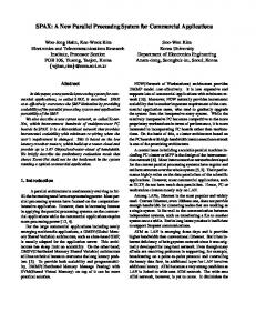
ability that the color was correctly reported was .715 (.736 when the stimuli differed in color). The corresponding probabilities that the orientation and the color were erroneously reported were .40 and .28, respectively, and the probabilities that no report was attempted were .01 and .01. We found a substantial proportion of trials on which just one feature from each of the two stimulus letters was reported correctly (see Figure 1). Across the 6 participants, the proportion of trials of this type ranged between .051 and .32 with a median of .19. Assuming that the four features are processed mutually independently, the probabilities of each of the 16 (i.e., 24) possible combinations of correctly and not correctly reported features (see Table 2) can be predicted from the observed (marginal) probabilities of correct report of each of the four features. For example, for a given participant, the probability of correct report of both the orientation and the color of the left-hand bar and the orientation but not the color of the right-hand bar (Report Type 12 in Table 2) should equal the product of (a) the (overall) probability (for the given participant) of correct report of the orientation of the lefthand bar, (b) the probability of correct report of the color of the left-hand bar, (c) the probability of correct report of the orientation of the right-hand bar, and (d) the complement of the probability of correct report of the color of the right-hand bar. Figure 2 shows graphs of observed and predicted probability distributions for the 16 different response types for each of the 6 participants under the assumption of mutually independent processing. As can be seen from the graphs, many of the participants showed strikingly close fits between the observed and theoretically predicted probabilities assuming identification of the four features to be mutually independent. Calculations of product–moment correlations between observed and predicted probabilities yielded values larger than .90

0.40 0.35

0 stimuli 1 stimulus 2 stimuli

Proportion of Trials

0.30 0.25 0.20 0.15 0.10 0.05 0.00 0

1

2

3

4

Correctly Reported Features Figure 1. Observed probability distribution of the number of correctly reported features in Experiment 1. The solid bar represents cases in which no features were correctly reported, open bars represent cases in which features from just one stimulus were reported correctly, and hatched bars represent cases in which one or more features from both stimuli were reported correctly.

PARALLEL PROCESSING

Table 2 Possible Types of Report in Experiments 1 and 2 Left Type

Feature 1

1 2 3 4 5 6 7 8 9 10 11 12 13 14 15 16

0 1 0 0 0 1 0 1 0 1 0 1 1 1 0 1

a

Right a

a

Feature 2

Feature 1

Feature 2a

0 0 1 0 0 1 0 0 1 0 1 1 1 0 1 1

0 0 0 1 0 0 1 1 0 0 1 1 0 1 1 1

0 0 0 0 1 0 1 0 1 1 0 0 1 1 1 1

Note. In Experiment 1, Features 1 and 2 were orientation and color, respectively. In Experiment 2, Features 1 and 2 were direction of motion and color, respectively. a 1 ⫽ correctly reported; 0 ⫽ not correctly reported.

(range ⫽ .934 –.987) for all 6 participants (see values in each panel of Figure 2). The square of the product–moment correlation between the observed and predicted probabilities is the proportion of variance in the observed probabilities that can be accounted for by the predicted probabilities (Winer, Brown, & Michels, 1991, p. 916). Given the correlations in Figure 2, the values for the 6 participants ranged between 87% and 97%. To verify the assumption of mutual independence of identification, a multinomial test of the correspondence between observed and predicted probabilities was performed for each participant using Monte Carlo simulations (see Appendix A). The resulting p values for each of the 6 participants are listed in Figure 2. The deviations of the observed probabilities from the probabilities predicted by assuming mutual independence were nonsignificant at a .05 level for 4 out of the 6 participants. For 2 of these 4 participants, the p values exceeded .50. To test the robustness of the conjecture of independent processing of the four features, we further analyzed the results of Experiment 1 by looking for evidence against independent processing either within each stimulus (objectwise analyses) or between the two stimuli but separately for each feature (featurewise analyses). In the objectwise analyses, the data were fitted separately for each of the two stimuli. The upper four panels of Figure 3 show observed and predicted probabilities for each of the two stimuli based on the marginal probabilities of the four features to be reported for two representative participants (S2 and S4). The four (22) different combinations of correctly and not correctly reported features from each stimulus are listed in Table 3. The product–moment correlations between observed and predicted probabilities ranged between .969 and 1.000 for the left stimulus and .948 and 1.000 for the right stimulus, thus accounting for 94%–100% and 90%–100% of the variance, respectively. Owing to the small number of different response types, it was feasible to run exact versions of the multinomial tests comparing

67

the observed and predicted probability distributions. Among the 6 participants, 5 participants showed no significant deviation between observed and predicted probabilities for the left-hand stimulus and 3 showed no significant deviation for the right-hand stimulus at a .05 level of significance. As many as 7 out of the 12 p values exceeded .50. In the featurewise analyses, the data were fitted within each of the two feature dimensions (orientation and color). The lower four panels of Figure 3 show observed and predicted probabilities for the two feature dimensions based on the marginal probabilities of the four features to be reported. The four (22) different combinations of correctly and not correctly reported features from the two stimuli are listed in Table 4. The product–moment correlations ranged between .939 and 1.000 for orientation and between .994 and 1.000 for color, thus accounting for 88%–100% and 99 –100% of the variance, respectively. The multinomial tests comparing the observed and predicted probability distributions yielded p values above .05 for 5 of the 6 participants’ reports of orientation and for all of the 6 participants’ reports of color. As many as 8 of the 12 p values exceeded .50. In the terminology proposed by Sperling and Speelman (1970), the analyses we have reported so far were based on position scores (numbers of features reported correctly with respect to both their identities and their locations). Let the identity score with respect to color or orientation be the position score that would be obtained if, before scoring, the locations of the colors or orientations, respectively, were permuted so as to maximize the position score. Mislocalizations of presented colors or orientations (illusory conjunctions; Treisman & Schmidt, 1982) should increase the identity scores relative to the position scores. In general, however, the identity score for each feature was only slightly higher than the corresponding position score. Averaged across participants, the position scores were 1.43 colors and 1.18 orientations per trial. The corresponding identity scores were 1.47 colors and 1.25 orientations per trial. To analyze the cause of the illusory conjunctions, we compared the observed identity scores with identity scores predicted by a model assuming independent parallel processing combined with random guessing (see Appendix B): For each feature, the probability of correct report (Pc) and the probability of an erroneous report (Pe) were assumed to result from a two-stage process. The first stage is the perceptual identification of the feature, which succeeds with probability P. If successful, the participant reports the feature at the correct location. If the perceptual identification process fails, a second guessing stage is engaged with probability Pg. At this stage the participant guesses randomly at the feature. The probability of guessing a feature at a given location correctly is 1/Nf, where Nf is the number of different categories within the feature dimension (6 for both the orientation and the color dimensions). The derivation of the unknown probabilities P and Pg is described in Appendix B. Averaged across participants and stimuli, probability P was .66 for color and .51 for orientation, whereas probability Pg was .97 for color and .94 for orientation. By Monte Carlo simulations (10,000 iterations per run) using probabilities P and Pg, we computed the predicted identity scores for each of the two features and each of the 6 participants. The observed identity score was then plotted against the corresponding predicted identity score for each feature and each participant (see Figure 4). A linear regression analysis of the observed identity

KYLLINGSBÆK AND BUNDESEN

68

0.5

0.6

S1

r = .987 p < .001

0.4 0.3

Observed Predicted

0.2

0.4 Proportion of Trials

Proportion of Trials

0.5

0.1

0.3 0.2 0.1

1 2 3 4 5 6 7 8 9 10 11 12 13 14 15 16

1 2 3 4 5 6 7 8 9 10 11 12 13 14 15 16

Type of Report

Type of Report

0.20

0.20

S3

0.18

r = .965 p = .505

0.16 0.14 0.12 0.10 0.08 0.06 0.04

S4

r = .962 p = .650

0.16 Proportion of Trials

Proportion of Trials

r = .979 p = .097

0.0

0.0

0.18

S2

0.14 0.12 0.10 0.08 0.06

0.02

0.04

0.00

0.02 0.00 1 2 3 4 5 6 7 8 9 10 11 12 13 14 15 16

1 2 3 4 5 6 7 8 9 10 11 12 13 14 15 16

Type of Report

Type of Report

0.30

S5

r = .938 p = .188

0.25 Proportion of Trials

Proportion of Trials

0.25

0.30

0.20 0.15 0.10 0.05 0.00

S6

r = .934 p = .045

0.20 0.15 0.10 0.05 0.00

1 2 3 4 5 6 7 8 9 10 11 12 13 14 15 16

1 2 3 4 5 6 7 8 9 10 11 12 13 14 15 16

Type of Report

Type of Report

Figure 2. Observed and predicted probability distributions for reports of pairs of colored bars across 16 types of report in Experiment 1. Panels S1–S6 represent the results for Participants S1–S6. Each panel also includes the correlation coefficient, r, between observed and predicted probabilities across the 16 possible types of report and the p value obtained by the multinomial test comparing predicted and observed probabilities across the 16 types of report. Report Types 1, 2–5, 6 –11, 12–15, and 16 stand for 0, 1, 2, 3, and 4 features correctly reported, respectively.

score as a function of the predicted identity score yielded a zero intercept of 0.11 and a slope of 0.94. The correlation coefficient was .998.

Discussion The results of Experiment 1 agreed very well with predictions by a simple parallel-processing model assuming stochastically

independent processing of features both within and between the two stimuli (see Figure 2). In particular, the results showed strong evidence of states of partial information from each of the two stimuli (states in which just one feature could be reported from each stimulus), and the probabilities of these states conformed to predictions by the independent parallel model. One might speculate that splitting the set of 216 trials for each participant across as many as 16 types of report could have masked

1.0

Proportion of trials

0.8

S2 Left

S4 Left

r = 1.000 p = 0.893

r = 0.977 p = 0.531

0.6 0.4 0.2 0.0

1.0

Proportion of trials

0.8

r = 0.979 p = 0.016

S2 Right

S4 Right

r = 0.996 p = 0.891

0.6 0.4 0.2 0.0

1.0

Proportion of trials

0.8

S4 Orientations

S2 Orientations

0.6

r = 0.999 p = 0.985

r = 1.000 p = 0.811

0.4 0.2 0.0

1.0

Proportion of trials

0.8

S2 Colors

r = 0.994 p = 0.462

S4 Colors

0.6

r = 1.000 p = 1.000

Observed Predicted

0.4 0.2 0.0 1

2

3

Type of Report

4

1

2

3

4

Type of Report

Figure 3. Observed and predicted probability distributions for different types of reports by two representative participants (S2 and S4) in Experiment 1. Each panel includes the correlation coefficient, r, between observed and predicted probabilities across the four possible types of report and the p value obtained by the multinomial test comparing predicted and observed probabilities across the four types of report. First row: Reports of features from the left stimulus. Report Types 1, 2, 3, and 4 stand for (a) neither orientation nor color correct, (b) just orientation correct, (c) just color correct, and (d) both orientation and color correct, respectively. Second row: Reports of features from the right stimulus (with types the same as for the left stimulus). Third row: Reports of the orientations of the two colored bars. Report Types 1, 2, 3, and 4 stand for (a) neither left nor right stimulus correct, (b) just left stimulus correct, (c) just right stimulus correct, and (d) both left and right stimuli correct, respectively. Fourth row: Reports of the colors of the two colored bars (with types the same as for orientation).

KYLLINGSBÆK AND BUNDESEN

70

small but systematic deviations from independent processing. However, analysis of the data separately both within stimuli (objectwise analyses) and between stimuli (featurewise analyses) showed no such systematic deviations from independence (see Figure 3). Thus, the analyses corroborated the conclusion that the four features (two colors and two orientations) of a stimulus pair were processed very nearly independently of each other. Mislocalizations of features (illusory conjunctions of orientations or colors with locations) were rare. Identity scores were only slightly higher than position scores. Furthermore, the identity scores were closely predicted by a model assuming independent parallel processing with perfect localization of features identified during perception combined with random guessing on some of those trials on which the perceptual feature identification failed (see Figure 4). Obviously, the assumption of perfect localization of features identified during perception is very strong and unlikely to be true in general. The generality of our model for illusory conjunctions must be limited to cases in which the locations of the stimuli are relatively far from each other. The results of Experiment 1 are hard to reconcile with a simple serial model, which assumes that all processing of one object is completed before the processing of the next object is commenced. In the context of the present experiment, the simple serial model predicts that both color and orientation of one of the stimuli are processed before processing of the color and the orientation of the second stimulus is begun. Reports containing just one feature from each of the two stimuli could occur if a feature was erroneously encoded, an encoded feature was forgotten, or a guess was made, but such events should be exceptions. However, the results showed that all observers gave many reports containing just one feature from each of the two stimuli: both orientations (Report Type 8 in Figure 2), both colors (Report Type 9), or even the orientation of one of the stimuli and the color of the other one (Report Types 10 and 11). Even more striking, the frequency of these and other types of report corresponded very closely to the frequencies predicted from the observed marginal probabilities of reporting each of the four relevant features by assuming stochastically independent processing both within and between the two stimuli. This finding seems incompatible with the simple serial model. Could the simple serial model be modified to predict stochastic independence between the four features (two colors and two orientations) of the stimulus pairs? Assume that instead of completing processing of one of the stimuli before processing of the other one is begun, the time spent on the first stimulus is kept constant across trials. A participant in Experiment 1 might, for example, spend

Table 3 Possible Types of Report for a Given Object Type

Feature 1a

Feature 2a

1 2 3 4

0 1 0 1

0 0 1 1

Note. In Experiment 1, Features 1 and 2 were orientation and color, respectively. In Experiment 2, Features 1 and 2 were direction of motion and color, respectively. In Experiment 3, Features 1 and 2 were shape and color, respectively. a 1 ⫽ correctly reported; 0 ⫽ not correctly reported.

Table 4 Possible Types of Report for a Given Feature in Experiments 1 and 2

a

Type

Left stimulusa

Right stimulusa

1 2 3 4

0 1 0 1

0 0 1 1

1 ⫽ correctly reported; 0 ⫽ not correctly reported.

60% of the available processing time on the first stimulus and 40% of the time on the second stimulus, regardless of whether and when the participant identifies any features of the first stimulus. If (a) the available processing time is constant across trials, (b) order of processing is fixed (e.g., left to right), and (c) features belonging to the same stimulus are processed independently, then the modified serial model predicts the same results as the model assuming mutually independent parallel processing of all four features. Note that any variation in the order of processing from trial to trial would induce positive correlations between features belonging to the same stimulus and negative correlations between features belonging to different stimuli. In general, any variation in the time spent, say, on the left-hand stimulus should induce a positive correlation between the two features of this stimulus. Also, if the time spent on the right-hand stimulus varies inversely with the time spent on the left-hand stimulus (e.g., the sum of the two processing times might equal the total exposure duration), any variation in the time spent on the left-hand stimulus also should induce a positive correlation between the two features of the right-hand stimulus as well as negative correlations between features from different stimuli.2,3

2 The performance predicted by the modified serial model can be simulated by actually presenting the two stimuli sequentially (and postmasked), forcing processing to be sequential. We found it instructive to demonstrate the predictions this way. 3 Referring to findings by Luck, Hillyard, Mangun, and Gazzaniga (1989), Mu¨ller, Malinowski, Gruber, and Hillyard (2003), and, in particular, Alvarez and Cavanagh (2005), an anonymous reviewer suggested that independent parallel processing may obtain for stimuli presented to different hemispheres (left vs. right) but not for stimuli presented to the same hemisphere. We tested this conjecture in a control study with stimulus displays showing two objects in the same visual hemifield (left or right), one above and one below the horizontal meridian. The design was similar to that of Bundesen et al. (2003), but trials were blocked by condition such that in one condition, the stimuli (colored letters) were presented to the left of fixation, and in the other condition, the stimuli were presented to the right of fixation. Proper fixation was monitored via an infrared video camera setup. The results conformed to predictions by the assumption of independent parallel processing. By our multinomial tests using Monte Carlo simulations, none of the 5 participants showed even marginally significant deviations between observed and predicted probabilities in either the left or the right hemifield (in each case, p ⬎ .10). Five of the 10 tests yielded p values above .50.

PARALLEL PROCESSING

71

Experiment 1

Experiment 2 3.0

3.0 Orientation Color

2.5

2.5

2.0

Observed

Observed

2.0

1.5

1.5

1.0

1.0

0.5

0.5

0.0

Motion (short) Color (short) Motion (medium) Color (medium) Motion (long) Color (long)

0.0 0.0

0.5

1.0

1.5

2.0

2.5

3.0

0.0

0.5

1.0

Predicted

2.0

2.5

3.0

2.5

3.0

Predicted

Experiment 3

Bundesen et. al. (2003)

3.0

3.0 Shape Color

2.5

Shape Color

2.5

2.0

Observed

2.0

Observed

1.5

1.5

1.5

1.0

1.0

0.5

0.5

0.0

0.0 0.0

0.5

1.0

1.5

2.0

2.5

3.0

0.0

Predicted

0.5

1.0

1.5

2.0

Predicted

Figure 4. Scatter plots comparing observed and predicted mean identity scores in each of four experiments (the current Experiments 1, 2, and 3 as well as the experiment of Bundesen et al., 2003). In each panel, the diagonal line indicates perfect correspondence between observed and predicted values. For Experiment 2, exposure duration is indicated by symbol shape.

Experiment 2: Motion and Color From Two Stimuli, Varying Exposure Duration In Experiment 2, the validity of the modified serial model was tested by using three different exposure durations. The order of trials with different exposure durations was randomized so that it was impossible for participants to predict the exposure duration of the two stimuli in any given trial. To further extend our findings from previous experiments, we included stimulus motion as one of

the relevant features. Participants were presented with two colored disks that moved independently of each other in one of eight different directions. The participant’s task was to report the color and the direction of motion of each of the two stimuli.

Method Participants. Six students and employees from the University of Copenhagen participated in the experiment. The mean age of the partici-

KYLLINGSBÆK AND BUNDESEN

Results Averaged across participants and stimuli (left vs. right) at short, medium, and long exposure durations, respectively, the probability that the motion of a stimulus was correctly reported was .14, .46, and .88 (.14, .46, and .87 when the two stimuli differed in direction of motion), and the probability that the color was correctly reported was .35, .65, and .81 (.35, .65, and .80 when the stimuli differed in color). The corresponding values of the probability that the motion was erroneously reported were .66, .51, and .12, in that order, and the corresponding values of the probability that the color was erroneously reported were .60, .34, and .19. Thus, at short, medium, and long exposure durations, respectively, the probability that no report of the motion of a stimulus was attempted was .20, .03, and .00, and the probability that no report of the color of a stimulus was attempted was .05, .01, and .00. Figure 5 shows the observed probability distributions of the number of correctly reported features. The data are shown in three panels (Panels A–C), one for each of the three exposure durations used. Again we found many trials on which only one feature from each of the two stimuli was reported correctly (Report Types 8 –11; see Table 2). The median proportions across the 6 participants were .16, .25, and .06 for short, medium, and long exposure durations,

0.6

Proportion of Trials

0.5

A

0 stimuli 1 stimulus 2 stimuli

0.4 0.3 0.2 0.1 0.0 0

1

2

3

4

Correctly Reported Features 0.6 0.5 Proportion of Trials

pants was 29 years (range ⫽ 24 –35 years). All participants had normal or corrected-to-normal visual acuity. Four of the participants were naive with respect to the purpose of the study. Stimuli. The stimulus material consisted of colored disks with a diameter of 12 mm (0.85° of visual angle). Eight different colors were used: red, yellow, green, blue, purple, cyan, brown, and gray (see Table 1 for CIE x, y coordinates). Each disk could move in one of eight different directions (N, NE, E, SE, S, SW, W, or NW). The speed of the disks was kept constant at a rate of 30 mm/s (⬃2°/s). A stationary mask was constructed by superimposing drawings in white (CIE x, y coordinates of .277/.328; 76.4 cd/m2) of the longest paths of motion (trajectories) in each of the eight possible directions. As in the prior experiment, all stimuli were presented on a black (0.0 cd/m2) background. Procedure. The general procedure was the same as in Experiment 1. The two disks initially appeared 80 mm (5.7°) to the left and right of fixation, respectively, each disk moving in one of the eight directions. After the disks had moved, two stationary masks covering all of the eight possible trajectories were presented, centered on the initial positions of the two disks. Before the actual experiment, participants were taught to designate the eight possible directions by numbers 1 to 8. Design. Each of the eight colors and directions of motion appeared equally often to the left and to the right of fixation in each block of 192 trials. Otherwise, the four critical features of a stimulus pair were chosen at random, independently of each other. There were no constraints on whether the direction of motion or the color could be the same for the two stimuli presented on a trial. Three different exposure durations (motion times) were used. The exposure durations were calibrated for each participant during the practice session to prevent ceiling and floor effects. The durations were chosen so that the difference between the short and the medium exposure duration was 28 ms (two screen refreshes) and the difference between the short and the long exposure duration was 69 ms (five refreshes). The selected short exposure duration was 74 ms for one participant and 46 ms for the remaining participants. As with color and direction of motion, the exposure duration was randomized across trials within each block of trials. Each of 2 participants ran a total of 576 trials (3 blocks of 192 trials); each of the remaining 4 participants ran a total of 384 trials (2 blocks of 192 trials). The day before the actual experiment, a practice session was run comprising 100 trials to familiarize the participant with the procedure.

B

0.4 0.3 0.2 0.1 0.0 0

1

2

3

4

Correctly Reported Features 0.6 0.5 Proportion of Trials

72

C

0.4 0.3 0.2 0.1 0.0 0

1

2

3

4

Correctly Reported Features

Figure 5. Observed probability distributions of the number of correctly reported features in Experiment 2. Panels A–C show the results obtained with short, medium, and long exposure durations, respectively. The solid bars represent cases in which no features were reported correctly, open bars represent cases in which features from just one stimulus were reported correctly, and hatched bars represent cases in which one or more features from both stimuli were reported correctly.

respectively. The corresponding ranges were .08 –.23, .17–.30, and .03–.10. The marginal probabilities of reporting each of the four relevant features (two colors and two directions of motion) were calculated for each of the 6 participants in each of the three different exposure

PARALLEL PROCESSING

Proportion of Trials

0.3

A

Observed Predicted r = .982 p = .432

0.2

0.1

0.0 1 2 3 4 5 6 7 8 9 10 11 12 13 14 15 16 Type of Report 0.2 r = .974 p = .518

Proportion of Trials

B

0.1

0.0 1 2 3 4 5 6 7 8 9 10 11 12 13 14 15 16 Type of Report

0.8 r = 1.000 p = .263

C Proportion of Trials

duration conditions and used to compute predicted probability distributions as in Experiment 1. The correspondence between observed and predicted probability distributions is shown for a representative participant with short, medium, and long exposure durations, respectively, in Figure 6. As in the previous experiment, we found strikingly good fits to the observed distributions. Across all combinations of participants and exposure durations, the product–moment correlations between the observed and the predicted probability distributions ranged between .813 and 1.00 (i.e., accounting for 66.0%–99.9% of the variance in the observed data), with a median of .983. At the .05 level of significance, the multinomial tests gave nonsignificant p values for all three exposure duration conditions in 4 participants, just one significant p value for a 5th participant, and significant p values for two of the three conditions in the last participant. Of the 18 tests, 8 yielded p values above .50. As in the analysis of Experiment 1, we further tested the assumption of independent processing by analyzing the data separately within each stimulus (objectwise analyses) and between the two stimuli for each feature (featurewise analyses) using the types of report defined in Tables 3 and 4. The results for a representative participant are shown in Figure 7. In the objectwise analyses of performance with the left-hand stimulus, the correlations between observed and predicted report probabilities ranged between .982 and 1.000 (96%–100% of the variance accounted for), .950 and 1.000 (90%–100%), and .999 and 1.000 (100%–100%) for the short, medium, and long exposure durations, respectively. For the right-hand stimulus, the corresponding correlations ranged between .996 and 1.000 (99%– 100%), .982 and 1.000 (96%–100%), and .999 and 1.000 (100%– 100%). Surprisingly, at the .05 level of significance, no participants showed significant deviations between the observed and predicted values at any of the three exposure durations for either the left- or the right-hand stimulus. A total of 32 of the 36 p values were above .50. In the featurewise analyses of reports of motion, the correlations between observed and predicted report probabilities ranged between .983 and 1.000 (97%–100% of the variance accounted for), .735 and .993 (54%–99%), and .979 and 1.000 (96%–100%) for the short, medium, and long exposure durations, respectively. For reports of color, the corresponding correlations ranged between .808 and .999 (65%–100%), .813 and 1.000 (66%–100%), and .995 and 1.000 (99%–100%) for the short, medium, and long exposure durations. Four of the 6 participants showed nonsignificant results at every exposure duration for both motion and color. A total of 32 of the 36 p values were above .05, and 25 of the p values exceeded .50. Identity and position scores were calculated for color and direction of motion at each of the three exposure durations. The identity scores were only moderately higher than the corresponding position scores. Averaged across participants, the position and identity scores were 0.27 (SD ⫽ 0.06) and 0.41 (SD ⫽ 0.05) for motion and 0.68 (SD ⫽ 0.22) and 0.81 (SD ⫽ 0.18) for color at the short exposure duration. At the medium exposure duration, the position and identity scores averaged 0.92 (SD ⫽ 0.30) and 1.02 (SD ⫽ 0.25) for motion and 1.30 (SD ⫽ 0.22) and 1.34 (SD ⫽ 0.19) for color. Finally, at the long exposure duration, the position and identity scores averaged 1.75 (SD ⫽ 0.09) and 1.78 (SD ⫽ 0.08) for motion and 1.61 (SD ⫽ 0.10) and 1.63 (SD ⫽ 0.09) for color.

73

0.6

0.4

0.2

0.0 1 2 3 4 5 6 7 8 9 10 11 12 13 14 15 16 Type of Report

Figure 6. Observed and predicted probability distributions for reports of pairs of moving colored disks across 16 types of report by a representative participant (Participant S1) in Experiment 2. Panels A–C show the results obtained with short, medium, and long exposure durations, respectively. Each panel includes the correlation coefficient, r, between observed and predicted probabilities across the 16 possible types of report and the p value obtained by the multinomial test comparing predicted and observed probabilities across the 16 types of report. Report Types 1, 2–5, 6 –11, 12–15, and 16 stand for 0, 1, 2, 3, and 4 features correctly reported, respectively.

As in Experiment 1, the observed identity scores were closely predicted by the model assuming independent parallel processing combined with random guessing (see Figure 4). Averaged across participants and stimuli, the perceptual identification probability P

KYLLINGSBÆK AND BUNDESEN

74 1.0

A

rl = 1.000 pl = 1.000 rr = 0.998 pr = 0.700

D

B

rl = 0.997 pl = 0.851 rr = 0.996 pr = 0.917

E

0.5

rm = 1.000 pm = 0.997 rc = 0.935 pc = 0.727

0.0

Proportion of Trials

1.0

0.5

rm = 0.735 pm = 0.805 rc = 0.999 pc = 0.812

0.0

1.0

C

F

rl = 1.000 pl = 0.986 rr = 1.000 pr = 0.997

0.5

rm = 1.000 pm = 0.571 rc = 0.999 pc = 0.383

0.0 1

2

3

Type of Report

4

1

2

3

4

Type of Report

Figure 7. Observed and predicted probability distributions for different types of reports by a representative participant (S1) in Experiment 2. Panels A–C show the results obtained with short, medium, and long exposure durations, respectively, separately for each of the two stimuli. Each panel shows results from both stimuli. Observed probabilities are shown by circles (left stimulus) and triangles (right stimulus). Predicted probabilities are indicated by unmarked points connected with unbroken lines (left stimulus) and dashed lines (right stimulus). Each panel includes the correlations rl (left stimulus) and rr (right stimulus) between observed and predicted probabilities across the four possible types of report and p values pl (left stimulus) and pr (right stimulus) obtained by the multinomial tests comparing predicted and observed probabilities across the four types of report. Report Types 1, 2, 3, and 4 stand for (a) neither motion nor color correct, (b) just motion correct, (c) just color correct, and (d) both motion and color correct, respectively. Panels D–F show the results obtained with short, medium, and long exposure durations, respectively, separately for motion and color. Each panel shows results for both features. Observed probabilities are shown by circles (motion) and triangles (color). Predicted probabilities are indicated by unmarked points connected with unbroken lines (motion) and dashed lines (color). Each panel includes the correlations rm (motion) and rc (color) between observed and predicted probabilities across the four possible types of report and p values pm (motion) and pc (color) obtained by the multinomial tests comparing predicted and observed probabilities across the four types of report. Report Types 1, 2, 3, and 4 stand for (a) neither left nor right stimulus correct, (b) just left stimulus correct, (c) just right stimulus correct, and (d) both left and right stimuli correct, respectively.

PARALLEL PROCESSING

at short, medium, and long exposure durations, respectively, was .05, .39, and .86 for motion and .26, .60, and .78 for color. The corresponding values of the guessing probability Pg were .78, .93, and .98 for motion and .93, .97, and .99 for color, respectively. A linear regression analysis of the observed identity score as a function of the identity score predicted by the model yielded an intercept of 0.002 and a slope of 1.01. The overall correlation coefficient between observed and predicted values was .998. Finally, we compared the development of the marginal probabilities across the three different exposure durations. As shown in Figure 8, an increase in exposure duration resulted in a corresponding increase in the marginal probabilities for both the left and the right stimuli.

Discussion The results of Experiment 2 showed clear evidence in 4 of the 6 participants of essentially perfect stochastic independence between encoding of each of the four stimulus features (two colors and two directions of motion) at each of the three exposure durations. Also, the observed identity scores were predicted very closely by our model assuming independent parallel processing with perfect localization of features identified during perception combined with random guessing on some of those trials on which the perceptual feature identification failed. If the data obtained with a single exposure duration (short, medium, or long) were considered separately, the stochastic independence we observed might be explained by the modified serial model in which the processing time spent on the first stimulus is kept constant across trials, regardless of whether and when the observer identifies any features of the first stimulus. Given that (a) the available processing time for a stimulus pair is constant across trials, such that both the time spent on the first stimulus and the

75

time spent on the second stimulus are constant across trials; (b) order of processing is fixed (or exactly the same length of time is spent on each of the two stimuli); and (c) features belonging to the same stimulus are processed independently, the modified serial model predicts mutually independent processing of all four features. However, in Experiment 2, the exposure duration varied from trial to trial. Because the variation was unpredictable, the participant could not adjust the processing time spent on the first stimulus to the exposure duration of the stimulus pair. In this situation, any trial-to-trial variations in the time spent on the first stimulus would induce positive correlations (within the affected exposure duration conditions) between features belonging to the same stimulus and negative correlations between features belonging to different stimuli. Keeping constant the time spent on the first stimulus combined with a fixed order of processing would make performance on either the left- or the right-hand stimulus independent of exposure duration, contrary to the actual results (see Figure 8). Keeping constant the time spent on the first stimulus but varying the order of processing would again induce positive correlations between features belonging to the same stimulus and negative correlations between features belonging to different stimuli. Thus, the results of Experiment 2 seem incompatible not only with the simple serial model but also with the modified serial model. To account for the data of Experiment 2, a serial model must assume multiple shifts of processing between the two stimuli. If processing is shifted sufficiently rapidly to and fro, the serial model will mimic the predictions of the simple parallel model. The idea is similar to the procedure used in modern multitasking operating systems, in which the computer rapidly shifts between the active programs, giving the user an impression that many programs are running at the same time. Thus, at a macroscopic level, this rapid-shifting serial model behaves in a parallel manner.

Experiment 3: Shape and Color From Three Stimuli 1.0

There is considerable evidence to suggest that visual short-term memory (VSTM) has a storage capacity of about three to four objects (e.g., Cattell, 1885; Lee & Chun, 2001; Luck & Vogel, 1997; Shibuya & Bundesen, 1988; Sperling, 1960; but see also Alvarez & Cavanagh, 2004; Wilken & Ma, 2004). In Experiment 3, our aim was to investigate whether the assumption of independent parallel processing used to model the data of Experiments 1 and 2 would hold when the number of stimuli was increased beyond the two objects used in the previous experiments. We also wanted to test our random-guessing model for illusory conjunctions at a display set size greater than two. The task of the participants was to report both letter type and color of each of three letters (i.e., a total of six features).

Report Probability for Right Stimulus

Exposure duration Short Medium Long

0.8

0.6

0.4

0.2

Method 0.0 0.0

0.2

0.4

0.6

0.8

1.0

Report Probability for Left Stimulus Figure 8. Probability of correct report from the right stimulus plotted against the probability of correct report from the left stimulus at each of the three exposure durations for each of the two feature dimensions in each of the 6 participants in Experiment 2.

Participants. Six students and employees from the University of Copenhagen participated in the experiment. The mean age of the participants was 35 years (range ⫽ 25–53 years). All participants had normal or corrected-to-normal visual acuity. Two of the participants were naive with respect to the purpose of the study. Stimuli. The stimulus material consisted of colored capital letters. All letters of the English alphabet except W (25 in total) were used. The letters were printed in one of six different colors also used in Experiment 1 (see Table 1 for CIE x, y coordinates). The letters were presented on a black

76

KYLLINGSBÆK AND BUNDESEN

background (0.0 cd/m2). The mean width of the letters was 34 mm (2.4° of visual angle; range, 0.86°–3.0°), and the height of all letters was 54 mm (3.9°). A 48 mm (3.4°) by 64 mm (4.6°) rectangle composed of 3 ⫻ 3-mm gray squares in three different gray levels was used as a mask. The CIE x, y coordinates for the three different gray levels were .31/.28 at 1.0 cd/m2; .29/.28 at 2.5 cd/m2; and .29/.28 at 4.8 cd/m2. Procedure. The procedure was the same as in Experiments 1 and 2 except as noted. Each stimulus display showed three colored letters positioned at the perimeter of an imaginary circle centered at fixation with a radius of 48 mm (3.4° of visual angle). Letter 1 (the top letter) was located at the 12 o’clock position, Letter 2 (the leftmost letter) at half past 7 o’clock, and Letter 3 (the rightmost letter) at half past 4 o’clock. The exposure duration of the letters was calibrated for each participant in a practice session to prevent ceiling and floor effects. The calibrated exposure duration of the letters ranged between 29 ms and 43 ms across the 6 participants. The exposure duration of the three masks was 500 ms. Participants were asked to try to “pay equally much attention” to each of the three stimuli on each trial of the experiment. After the presentation, the participant verbally reported the color and the letter type of each of the three stimuli. Design. Each of the 25 letter types and each of the six colors were presented equally often at each of the three display positions. There were no constraints on whether letters in the same display could be the same in color or shape. Before the experiment was begun, participants were informed of the possible letter types and colors and informed that both letter types and colors were drawn with replacement for each trial. Each participant ran a total of 200 trials. Short breaks were held between blocks of 50 trials. The day before the actual experiment, a practice session was run comprising 100 trials to familiarize the participant with the procedure.

Results Performance was neither at ceiling nor at floor. Averaged across participants and stimuli, the observed probabilities that the shape (letter type) and the color of a stimulus were correctly reported were .49 and .71, respectively. The corresponding probabilities that the features were erroneously reported were .17 and .11, respectively, and the probabilities that no report was attempted were .34 and .18. On a considerable proportion of trials, participants gave reports containing just one feature from each of two of the three letters (median probability across the 6 participants ⫽ .10; range ⫽ .003–.17), one feature from each of the three letters (median ⫽ .06; range ⫽ .04 –.13), or two features from one letter and one feature from each of the two remaining letters (median ⫽ .16; range ⫽ .12–.32). Because only 200 trials were run for each participant, we did not analyze the data split across all 64 (26) different types of report. However, we tested for independence both within each stimulus (objectwise analyses) and between the stimuli but separately for each feature (featurewise analyses). In the objectwise analyses, the data were fitted separately for each of the three stimuli. Figure 9 shows observed and predicted probabilities for the top letter, the leftmost letter, and the rightmost letter, respectively, for a representative participant. The predictions are based on the marginal probabilities of the six features to be reported. The four (22) different combinations of correctly and not correctly reported features from each letter are listed in Table 3. The product–moment correlations between observed and predicted probabilities were high, but the fits were noticeably less good than the corresponding fits in Experiments 1 and 2. Across

participants, the correlations ranged between .869 and 1.00 for the top letter, .316 and .997 for the leftmost letter, and .748 and .998 for the rightmost letter, thus accounting for 76%–100%, 10%– 99%, and 56%–100% of the variance, respectively. Owing to the small number of different response types, we were again able to run exact versions of the multinomial tests comparing the observed and predicted probability distributions. Among the 6 participants, 3 participants showed no significant deviation between observed and predicted probabilities for the top letter, 2 showed no significant deviation for the leftmost letter, and 2 showed no significant deviation for the rightmost letter at a .05 level of significance. A total of 3 of the 18 p values were above .50. In the featurewise analyses, the data were fitted within each of the two feature dimensions (shape and color). Figure 10 shows observed and predicted probabilities for the two feature dimensions based on the marginal probabilities of the six features to be reported. The eight (23) different combinations of correctly and not correctly reported features from the three letters are listed in Table 5. The featurewise fits were good. The product–moment correlations ranged between .790 and .976 for shape and between .965 and .996 for color, thus accounting for 62%–95% and 93%–99% of the variance, respectively. The multinomial tests comparing the observed and predicted probability distributions were done via Monte Carlo simulations. The tests yielded p values above .05 for 4 of the 6 participants’ reports of shape and for all of the 6 participants’ reports of color. As many as 5 of the 12 p values were above .50. As in Experiments 1 and 2, the identity scores were not much higher than the corresponding position scores. Averaged across participants, the position and identity scores were 1.46 (SD ⫽ 0.34) and 1.53 (SD ⫽ 0.37) for shape and 2.14 (SD ⫽ 0.26) and 2.20 (SD ⫽ 0.23) for color. Also, as in Experiments 1 and 2, the observed identity scores were closely predicted by the model assuming independent parallel processing combined with random guessing (see Figure 4). Averaged across participants and stimuli, the perceptual identification probability P was .48 for shape and .69 for color, whereas the guessing probability Pg was .41 for shape and .43 for color. A linear regression analysis of the observed identity score as a function of the identity score predicted by the model yielded an intercept of 0.04 and a slope of 1.00. The correlation was .997.

Discussion To a first approximation, the results of Experiment 3 agreed reasonably well with predictions by the simple parallel-processing model assuming stochastically independent processing of features both within and between the three stimuli. In particular, the correspondence between observed and predicted values was good when considering independence of feature processing between the three stimuli (featurewise analyses; cf. Figure 10). However, by tests for independence of feature processing within each of the three stimuli (objectwise analyses; cf. Figure 9), the assumption of independent processing was violated in many of the participants. The violations appeared as overrepresentations of Report Types 1 and 4 and underrepresentations of Report Types 2 and 3 (cf. Table 3) relative to the predictions by the independent parallelprocessing model. In reports of Types 1 and 4, either none or both of the relevant features are reported correctly; in reports of Types

PARALLEL PROCESSING

77

0.7

A

Proportion of Trials

0.6 0.5

Observed Predicted

0.4

r = .998 p = .166

0.3 0.2 0.1 0.0

1

2

3

4

Type of Report

0.5

0.6

B

C

0.3

r = .983 p < .001

0.2 0.1

Proportion of Trials

Proportion of Trials

r = .985 p = .176

0.5

0.4

0.4 0.3 0.2 0.1

0.0

0.0 1

2

3

4

1

Type of Report

2

3

4

Type of Report

Figure 9. Observed and predicted probability distributions across four types of report of features from each of the three colored letters in Experiment 3. Data are for one representative participant (S1). Panels A, B, and C are for the top letter, the leftmost letter, and the rightmost letter, respectively. Each panel includes the correlation coefficient, r, between observed and predicted probabilities across the four types of report and the p value obtained by the multinomial test comparing predicted and observed probabilities across the four types of report. Report Types 1, 2, 3, and 4 stand for (a) neither shape nor color correct, (b) just shape correct, (c) just color correct, and (d) both shape and color correct, respectively.

2 and 3, only a single feature is reported correctly. Thus, the results showed positive correlations between reports of features belonging to the same stimulus. A plausible explanation for this finding is that the distribution of attention across the three stimuli may have varied somewhat from trial to trial. Keeping the distribution of attention (the relative attentional weights; Bundesen, 1990) constant across three stimuli should be more difficult than keeping it constant across two stimuli, and any variation in the distribution from trial to trial should induce positive correlations between reports of features from the same stimulus and negative correlations between reports of features from different stimuli. Despite the complexity of the task, one of the participants seemed able to comply very precisely with the instruction to keep a constant attentional set, showing clear evidence of independent parallel processing, similar to the data patterns found in Experiments 1 and 2. Thus, this participant seemed able to process a total

of six features, two from each of three stimuli, in parallel and perfectly independently. As in our experiments with stimulus pairs, mislocalizations of features (illusory conjunctions of shapes or colors with locations) were rare. Identity scores were not much higher than position scores, and they were fairly well predicted by a model assuming independent parallel processing with perfect localization of features identified during perception combined with random guessing on some of those trials on which the perceptual feature identification failed (see Figure 4).

General Discussion Summary Bundesen et al. (2003) presented observers with brief exposures of pairs of colored letters and asked them to report both the color

KYLLINGSBÆK AND BUNDESEN

78 0.4

Proportion of Trials

A 0.3

Observed Predicted

0.2

r = .976 p = .769

0.1

0.0 1

2

3

4

5

6

7

8

Type of Report

0.8

r = .994 p = .170

B Proportion of Trials

0.6

0.4

0.2

0.0

1

2

3

4

5

6

7

8

Type of Report Figure 10. Observed and predicted probability distributions for reports of the shapes (A) and colors (B) of the three letters across eight possible types of report in Experiment 3. Data are for Participant S1. Each panel includes the correlation coefficient, r, between observed and predicted probabilities across the eight types of report and the p value obtained by the multinomial test comparing predicted and observed probabilities across the eight types of report. Report Types 1, 2– 4, 5–7, and 8 stand for 0, 1, 2, and 3 objects correctly reported, respectively.

and the identity of each letter. Several participants showed clear evidence of nearly perfect stochastic independence between reports of the four features (two colors and two letter identities). In Experiment 1 of the present study, we replicated this finding with a stimulus material consisting of pairs of colored bars. The participants were asked to report both the color and the orientation of each bar, and the results agreed very well with predictions by a simple parallel-processing model assuming stochastically independent processing of features both within and between the two stimuli. In particular, the results showed strong evidence of states of partial information from each of the two stimuli (states in which just one feature could be reported from each stimulus), and the probabilities of these states conformed closely to predictions by the independent parallel model. Mislocalizations of features (illusory conjunctions of orientations or colors with locations) were rare. Identity scores were not much higher than position scores,

and the identity scores were closely predicted by a model assuming independent parallel processing with perfect localization of features identified during perception combined with random guessing on some of those trials on which the perceptual feature identification failed. By a simple serial model, “processing takes place on one element at a time, each element being completed before the next is begun” (Townsend & Ashby, 1983, p. 9). As regards Experiment 1, the simple model predicts that both the color and the orientation of one of the stimuli are encoded before either the color or the orientation of the other stimulus is encoded. There should be no trials on which the observer encodes just one feature from one of the stimuli and one feature from the other one. Contrary to this prediction, we found stochastic independence between reports of the four features. This finding seems incompatible with the simple serial model. To predict stochastic independence between the four features of a stimulus pair in Experiment 1, the serial model could be modified by assuming that instead of completing processing of one of the stimuli before processing of the other one is begun, the time spent on the first stimulus is kept constant, regardless of whether and when the observer identifies any features of the stimulus. In Experiment 2, we tested the modified serial model by varying exposure durations unpredictably from trial to trial. With a stimulus material consisting of pairs of colored moving disks, we found virtually perfect stochastic independence between reports of color and direction of motion of each of the two disks at each of the three levels of exposure duration. At the same time, performance improved for both stimuli as exposure duration was increased. As explained in the discussion of Experiment 2, this combination of results seems incompatible not only with the simple serial model but also with the modified serial model. The position scores found in Experiments 1 and 2 agreed closely with predictions by a model assuming that the four features of a stimulus pair were processed (identified and localized) in parallel and stochastically independently. Similarly, the identity scores were closely predicted by a model assuming independent parallel processing with perfect localization of features identified during perception combined with random guessing on some of those trials on which the perceptual feature identification failed. In Experiment 3, we tested the generality of our findings by presenting observers with triples of colored letters and asking them to report the color and the type of each of the three letters. To a first approximation, the position scores agreed reasonably well

Table 5 Possible Types of Report for a Given Feature (Shape or Color) in Experiment 3 Type

Letter 1a

Letter 2a

Letter 3a

1 2 3 4 5 6 7 8

0 1 0 0 1 1 0 1

0 0 1 0 1 0 1 1

0 0 0 1 0 1 1 1

a

1 ⫽ correctly reported; 0 ⫽ not correctly reported.

PARALLEL PROCESSING

with predictions by a model assuming that the six features of a stimulus pair were processed (identified and localized) in parallel and stochastically independently, and the identity scores agreed closely with the same model combined with random guessing on some of those trials on which the perceptual feature identification failed. However, the correspondence between observed and predicted probabilities was less close with the stimulus triples in Experiment 3 than with the stimulus pairs in our previous experiments. Just 1 of the 6 participants seemed able to process the set of six features, two from each of three stimuli, completely independently across trials. Apparently, when the display set size was increased from two to three stimulus objects, most participants were unable to keep the attentional weighting of the stimulus letters strictly constant from trial to trial.

Theoretical Implications Our findings are hard to reconcile with the feature integration theory of Treisman (1988, 1993, 1996; Treisman & Gelade, 1980; Treisman & Sato, 1990; Treisman & Schmidt, 1982) and the guided search model of Wolfe (1994, 1998; Cave & Wolfe, 1990; Wolfe, Cave, & Franzel, 1989). In both theories, simple stimulus features such as color and orientation are registered automatically, without attention, and in parallel across the visual field. However, registration of objects (items that are defined by conjunctions of features) requires a further stage of processing during which spatial attention is directed to one object at a time. Spatial attention is likened to a spotlight, and the function of directing attention to a particular location in space is to bind (link) all features at the attended location to each other as well as binding them to the location. Thus, localizing a feature requires spatial attention, and only one location can be attended at a time. This is hard to reconcile with the evidence we have provided that multiple features of each of two to three stimuli can be identified and localized in parallel. Our findings also bear on biased competition models of the type described by Desimone and Duncan (1995; Desimone, 1998; Duncan, 1996, 1998; Duncan, Humphreys, & Ward, 1997). In some implementations of biased competition, activation of a neural unit representing that a given object has a particular feature (e.g., object x is red) facilitates activation of units representing other, unrelated categorizations of the same object (e.g., object x moves upward) and inhibits activation of units representing (related or unrelated) categorizations of objects other than x. This is the integrated competition hypothesis of Duncan (1996); units representing categorizations of the same object reinforce each other while competing against units representing categorizations of other objects. The formulation suggests that trial-to-trial variations in whether a certain feature of a given object is reportable should be (a) positively correlated with variations in whether other features of the same object are reportable and (b) negatively correlated with variations in whether features of other objects are reportable. Our experiments show that this is not invariably so. In Experiments 1 and 2, trial-to-trial variations in whether a particular feature was correctly reported showed little or no dependence on whether (a) the other feature of the same object was correctly reported or (b) features of the other object were correctly reported. Our findings lend support to independent parallel-processing theories such as the unlimited-capacity theory of Palmer, Verghese, and Pavel (2000) and the limited-capacity theory of visual

79

attention called TVA (Bundesen, 1990; also see Bublak et al., 2005; Bundesen, 1991, 1998a, 1998b; Bundesen, Habekost, & Kyllingsbæk, 2005; Bundesen, Kyllingsbæk, Houmann, & Jensen, 1997; Duncan et al., 1999, 2003; Finke et al., 2005; Habekost & Bundesen, 2003; Hung, Driver, & Walsh, 2005; Kyllingsbæk, 2006; Kyllingsbæk, Schneider, & Bundesen, 2001). Formally, TVA may be regarded as another implementation of biased competition. In TVA, visual recognition and attentional selection consist in encoding visual categorizations of the form “object x has feature i” into VSTM. The storage capacity of VSTM is limited to about four different objects. The objects that become encoded into VSTM are those objects that first complete processing with respect to some categorization. Thus, the process of attentional selection is conceived as a parallel processing race. The time course of the race is stochastically modeled, such that the processing speed of the categorization “object x has feature i” is given by v共x,i兲 ⫽ ␩共x,i兲␤ i

wx

冘

,

(1)

wz

z僆S

where ␩(x,i) is the strength of the sensory evidence that supports the categorization, ␤i is the subject’s bias for ascribing feature i to objects, S is the set of all objects in the visual field, and wx and wz are attentional weights of objects x and z, respectively. By Equation 1, variation in the attentional weight of an object should generate positive correlation between probabilities of recognizing (selecting) different features of the given object but negative correlation between probabilities of recognizing features of the given object and recognizing features of other objects. However, if all processing parameters (␩, ␤, and w values) are kept constant, processing times for visual categorizations of different objects should be stochastically independent, as should processing times for functionally independent features of any given object. Thus, when attentional weights are kept constant, and VSTM capacity is not exceeded, stochastic independence should be found. If attentional weights are varied or VSTM capacity is exceeded, stochastic dependence should prevail. Whereas cases of perfect stochastic independence between reports of different objects may be rare, parallel identification of several objects from a given fixation may be the rule rather than the exception (cf. Bundesen, 1990; also see Awh & Pashler, 2000; Bichot, Cave, & Pashler, 1999; McMains & Somers, 2004, 2005). In general, however, an attention system capable of parallel processing with spatially selective allocation of processing resources is also capable of serial processing (Bundesen, 1990). The serial processing can be done by first using a spatial selection criterion for sampling objects from one part of the stimulus display, then shifting the selection criterion to sample objects from another part of the display, and so forth, with or without eye movements. Bundesen (1990) analyzed the efficiency of serial versus parallel search in terms of TVA. The analysis was based on the hypothesis that processing is optimized so that serial processing occurs when the time cost of shifting (reallocating) attention is outweighed by gain in speed of processing after attention has been shifted. For simplicity, let targets and distractors be equal in attentional weights, and consider search through a display consisting of two objects. If the objects are processed in parallel with a total capacity of C (objects per time unit), the mean time to the first completion of an object is C–1, and the mean time from the first to

KYLLINGSBÆK AND BUNDESEN

80

the second completion is (C/2)–1 ⫽ 2C–1. If processing is serial with a capacity of C, the mean time to the first completion is again C–1. The mean time from the first to the second completion is s ⫹ C–1, where s is the time taken to shift attention between objects. Therefore, to optimize performance, processing should be serial if, and only if, s ⬍ C–1. For example, if a shift of attention takes 100 ms, the two objects should be processed in series if, and only if, the mean time taken to process a singly presented object (C–1) is longer than 100 ms. Bundesen (1990) extended the above line of reasoning and considered the time cost of shifting attention to a group of n items and then processing the n items in parallel. The theoretical time cost per member of the group proved to be least if group size n equals the product of C and s or the smallest integer greater than Cs. Numerical calculations showed that typical data on slow feature (Treisman & Gormican, 1988) and conjunction (Treisman & Gelade, 1980) search could be explained by attention shifting among groups of stimulus objects such that processing is parallel within groups but serial between groups (cf. Bundesen & Pedersen, 1983; Pashler, 1987; Treisman, 1982). The more difficult the search, the smaller is the optimal group size. For example, if the time taken to shift attention (s) is 100 ms, and the total processing capacity (C) distributed over the n objects in a group is 100 objects/s, processing should be optimized at a group size of 10 objects. If the time taken to shift attention is 100 ms, but the total processing capacity is less than 10 objects/s, the optimal group size is only 1, so in this case only one object should be processed at a time (cf. Bricolo et al., 2002; also see Woodman & Luck, 1999).

References Allport, D. A. (1968). The rate of assimilation of visual information. Psychonomic Science, 12, 231–232. Alvarez, G. A., & Cavanagh, P. (2004). The capacity of visual short-term memory is set both by visual information load and by number of objects. Psychological Science, 15, 106 –111. Alvarez, G. A., & Cavanagh, P. (2005). Independent resources for attentional tracking in the left and right visual hemifields. Psychological Science, 16, 637– 643. Atkinson, R. C., Holmgren, J. R., & Juola, J. F. (1969). Processing time as influenced by the number of elements in a visual display. Perception & Psychophysics, 6, 321–326. Awh, E., & Pashler, H. (2000). Evidence for split attentional foci. Journal of Experimental Psychology: Human Perception and Performance, 26, 834 – 846. Bichot, N. P., Cave, K. R., & Pashler, H. (1999). Visual selection mediated by location: Feature-based selection of noncontiguous locations. Perception & Psychophysics, 61, 403– 423. Bricolo, E., Gianesini, T., Fanini, A., Bundesen, C., & Chelazzi, L. (2002). Serial attention mechanisms in visual search: A direct behavioral demonstration. Journal of Cognitive Neuroscience, 14, 980 –993. Bublak, P., Finke, K., Krummenacher, J., Preger, R., Kyllingsbæk, S., Mu¨ller, H. J., & Schneider, W. X. (2005). Usability of a theory of visual attention (TVA) for parameter-based measurement of attention: II. Evidence from two patients with frontal or parietal damage. Journal of the International Neuropsychological Society, 11, 843– 854. Bundesen, C. (1990). A theory of visual attention. Psychological Review, 97, 523–547. Bundesen, C. (1991). Visual selection of features and objects: Is location special? A reinterpretation of Nissen’s (1985) findings. Perception & Psychophysics, 50, 87– 89. Bundesen, C. (1998a). A computational theory of visual attention. Philo-

sophical Transactions of the Royal Society of London, Series B, 353, 1271–1281. Bundesen, C. (1998b). Visual selective attention: Outlines of a choice model, a race model, and a computational theory. Visual Cognition, 5, 287–309. Bundesen, C., & Habekost, T. (2005). Attention. In K. Lamberts & R. Goldstone (Eds.), Handbook of cognition (pp. 105–129). London: Sage. Bundesen, C., Habekost, T., & Kyllingsbæk, S. (2005). A neural theory of visual attention. Bridging cognition and neurophysiology. Psychological Review, 112, 291–328. Bundesen, C., Kyllingsbæk, S., Houmann, K. J., & Jensen, R. M. (1997). Is visual attention automatically attracted by one’s own name? Perception & Psychophysics, 59, 714 –720. Bundesen, C., Kyllingsbæk, S., & Larsen, A. (2003). Independent encoding of colors and shapes from two stimuli. Psychonomic Bulletin & Review, 10, 474 – 479. Bundesen, C., & Pedersen, L. F. (1983). Color segregation and visual search. Perception & Psychophysics, 33, 487– 493. ¨ ber die Zeit der Erkennung und Benennung SchriftCattell, J. M. (1885). U zeichen, Bildern und Farben [The time it takes to recognize and name letters, pictures, and colors]. Philosophische Studien, 2, 635– 650. Cave, K. R., & Wolfe, J. M. (1990). Modeling the role of parallel processing in visual search. Cognitive Psychology, 22, 225–271. Desimone, R. (1998). Visual attention mediated by biased competition in extrastriate visual cortex. Philosophical Transactions of the Royal Society of London, Series B, 353, 1245–1255. Desimone, R., & Duncan, J. (1995). Neural mechanisms of selective visual attention. Annual Review of Neuroscience, 18, 193–222. Duncan, J. (1984). Selective attention and the organization of visual information. Journal of Experimental Psychology: General, 113, 501–517. Duncan, J. (1993). Similarity between concurrent visual discriminations: Dimensions and objects. Perception & Psychophysics, 54, 425– 430. Duncan, J. (1996). Cooperating brain systems in selective perception and action. In T. Inui & J. L. McClelland (Eds.), Attention and performance XVI: Information integration in perception and communication (pp. 549 –578). Cambridge, MA: MIT Press. Duncan, J. (1998). Converging levels of analysis in the cognitive neuroscience of visual attention. Philosophical Transactions of the Royal Society of London, Series B, 353, 1307–1317. Duncan, J., Bundesen, C., Olson, A., Humphreys, G., Chavda, S., & Shibuya, H. (1999). Systematic analysis of deficits in visual attention. Journal of Experimental Psychology: General, 128, 450 – 478. Duncan, J., Bundesen, C., Olson, A., Humphreys, G., Ward, R., Kyllingsbæk, S., et al. (2003). Attentional functions in dorsal and ventral simultanagnosia. Cognitive Neuropsychology, 20, 675–701. Duncan, J., & Humphreys, G. W. (1989). Visual search and stimulus similarity. Psychological Review, 96, 433– 458. Duncan, J., Humphreys, G. W., & Ward, R. (1997). Competitive brain activity in visual attention. Current Opinion in Neurobiology, 7, 255–261. Eriksen, C. W., & Lappin, J. S. (1967). Independence in the perception of simultaneously presented forms at brief durations. Journal of Experimental Psychology, 73, 468 – 472. Finke, K., Bublak, P., Krummenacher, J., Kyllingsbæk, S., Mu¨ller, H. J., & Schneider, W. X. (2005). Usability of a theory of visual attention (TVA) for parameter-based measurement of attention: I. Evidence from normal subjects. Journal of the International Neuropsychological Society, 11, 832– 842. Grossberg, S., Mingolla, E., & Ross, W. D. (1994). A neural theory of attentive visual search: Interactions of boundary, surface, spatial, and object representations. Psychological Review, 101, 470 – 489. Habekost, T., & Bundesen, C. (2003). Patient assessment based on a theory of visual attention (TVA): Subtle deficits after a right frontal-subcortical lesion. Neuropsychologia, 41, 1171–1188. Hung, J., Driver, J., & Walsh, V. (2005). Visual selection and posterior

PARALLEL PROCESSING parietal cortex: Effects of repetitive transcranial magnetic stimulation on partial report analyzed by Bundesen’s theory of visual attention. Journal of Neuroscience, 25, 9602–9612. Kyllingsbæk, S. (2006). Modeling visual attention. Behavior Research Methods, 38, 123–133. Kyllingsbæk, S., Schneider, W. X., & Bundesen, C. (2001). Automatic attraction of attention to former targets in visual displays of letters. Perception & Psychophysics, 63, 85–98. Lee, D., & Chun, M. M. (2001). What are the units of visual short-term memory, objects or spatial locations? Perception & Psychophysics, 63, 253–257. Luck, S. J., Hillyard, S. A., Mangun, G. R., & Gazzaniga, M. S. (1989, November 30). Independent hemispheric attentional systems mediate visual search in split-brain patients. Nature, 342, 543–545. Luck, S. J., & Vogel, E. K. (1997, November 20). The capacity of visual working memory for features and conjunctions. Nature, 390, 279 –281. Magnussen, S., Greenlee, M., & Thomas, J. P. (1996). Parallel processing in visual short-term memory. Journal of Experimental Psychology: Human Perception and Performance, 22, 202–212. McMains, S. A., & Somers, D. C. (2004). Multiple spotlights of attentional selection in human visual cortex. Neuron, 42, 677– 686. McMains, S. A., & Somers, D. C. (2005). Processing efficiency of divided spatial attention mechanisms in human visual cortex. Journal of Neuroscience, 25, 9444 –9448. Monheit, M. A., & Johnston, J. C. (1994). Spatial attention to arrays of multidimensional objects. Journal of Experimental Psychology: Human Perception and Performance, 20, 691–708. Mu¨ller, M. M., Malinowski, P., Gruber, T., & Hillyard, S. A. (2003, July 17). Sustained division of the attentional spotlight. Nature, 424, 309 –312. Nissen, M. J. (1985). Accessing features and objects: Is location special? In M. I. Posner & O. S. M. Marin (Eds.), Attention and performance XI (pp. 205–219). Hillsdale, NJ: Erlbaum. Palmer, J., Verghese, P., & Pavel, M. (2000). The psychophysics of visual search. Vision Research, 40, 1227–1268. Pashler, H. (1987). Detecting conjunctions of color and form: Reassessing the serial search hypothesis. Perception & Psychophysics, 41, 191–201. Shibuya, H., & Bundesen, C. (1988). Visual selection from multielement displays: Measuring and modeling effects of exposure duration. Journal of Experimental Psychology: Human Perception and Performance, 14, 591– 600. Sperling, G. (1960). The information available in brief visual presentations. Psychological Monographs, 74(11, Whole No. 498). Sperling, G. (1963). A model for visual memory tasks. Human Factors, 5, 19 –31. Sperling, G. (1967). Successive approximations to a model for short term memory. Acta Psychologica, 27, 285–292. Sperling, G., & Speelman, R. G. (1970). Acoustic similarity and auditory short-term memory: Experiments and a model. In D. A. Norman (Ed.), Models of human memory (pp. 151–202). New York: Academic Press. Townsend, J. T. (1969). Mock parallel and serial models and experimental detection of these. In Purdue Centennial Symposium on Information Processing (pp. 617– 628). West Lafayette, IN: Purdue University.

81

Townsend, J. T. (1990). Serial vs. parallel processing: Sometimes they look like Tweedledum and Tweedledee but they can (and should) be distinguished. Psychological Science, 1, 46 –54. Townsend, J. T., & Ashby, F. G. (1983). Stochastic modeling of elementary psychological processes. Cambridge, England: Cambridge University Press. Townsend, J. T., & Evans, R. (1983). A systems approach to parallel–serial testability and visual feature processing. In H. G. Geissler (Ed.), Modern issues in perception (pp. 166 –189). Berlin, Germany: VEB Deutscher Verlag der Wissenschaften. Treisman, A. M. (1982). Perceptual grouping and attention in visual search for features and for objects. Journal of Experimental Psychology: Human Perception and Performance, 8, 194 –214. Treisman, A. M. (1988). Features and objects: The Fourteenth Bartlett Memorial Lecture. Quarterly Journal of Experimental Psychology: Human Experimental Psychology, 40(A), 201–237. Treisman, A. M. (1993). The perception of features and objects. In A. Baddeley & L. Weiskrantz (Eds.), Attention: Selection, awareness, and control (pp. 5–35). Oxford, England: Oxford University Press. Treisman, A. (1996). The binding problem. Current Opinion in Neurobiology, 6, 171–178. Treisman, A. M., & Gelade, G. (1980). A feature-integration theory of attention. Cognitive Psychology, 12, 97–136. Treisman, A. M., & Gormican, S. (1988). Feature analysis in early vision: Evidence from search asymmetries. Psychological Review, 95, 15– 48. Treisman, A. M., & Sato, S. (1990). Conjunction search revisited. Journal of Experimental Psychology: Human Perception and Performance, 16, 459 – 478. Treisman, A. M., & Schmidt, H. (1982). Illusory conjunctions in the perception of objects. Cognitive Psychology, 14, 107–141. van der Velde, F., & van der Heijden, A. H. C. (1997). On the statistical independence of color and shape in object identification. Journal of Experimental Psychology: Human Perception and Performance, 23, 1798 –1812. Vecera, S. P., & Farah, M. J. (1994). Does visual attention select objects or locations? Journal of Experimental Psychology: General, 123, 146 –160. Wilken, P., & Ma, W. J. (2004). A detection theory account of change detection. Journal of Vision, 4, 1120 –1135. Winer, B. J., Brown, D. R., & Michels, K. M. (1991). Statistical principles in experimental design. New York: McGraw-Hill. Wolfe, J. M. (1994). Guided search 2.0: A revised model of visual search. Psychonomic Bulletin & Review, 1, 202–238. Wolfe, J. M. (1998). What can 1 million trials tell us about visual search? Psychological Science, 9, 33–39. Wolfe, J. M. (2003). Moving towards solutions to some enduring controversies in visual search. Trends in Cognitive Sciences, 7, 70 –76. Wolfe, J. M., Cave, K. R., & Franzel, S. L. (1989). Guided search: An alternative to the feature integration model for visual search. Journal of Experimental Psychology: Human Perception and Performance, 15, 419–433. Woodman, G. F., & Luck, S. J. (1999, August 26). Electrophysiological measurement of rapid shifts of attention during visual search. Nature, 400, 867– 869.

(Appendixes follow)

KYLLINGSBÆK AND BUNDESEN

82

Appendix A A Multinomial Test for Mutually Independent Parallel Processing Here we present a multinomial test of the correspondence between observed and predicted probability distributions for the report types found in Experiments 1–3. Consider the analysis of Experiment 1 for Participant S1 as an example. The assumption of mutual independence between reports of the four features was evaluated for the participant by testing the hypothesis that the frequencies of the 16 types of report (see Table 2) followed a multinomial probability distribution for 216 trials, each with 16 possible outcomes, one for each of the 24 possible combinations of the results of four independent binary events (success or failure with respect to each of the four features). The hypothesis was tested by Monte Carlo computer simulations. First, the best fitting multinomial distribution was determined as the distribution with N ⫽ 216 trials, each with 16 possible outcomes with probabilities computed by treating the four observed marginal probabilities as the theoretical probabilities of the underlying four independent binary events. Second, the probability (q0) of the observed distribution of 216 reports across the 16 possible types of report was calculated by the multinomial probability law. Third, the participant’s run through 216 trials was simulated 106 times. On each of the 106 iterations, a distribution of 216 reports across the 16

possible types was generated, and the probability (qs) of the generated distribution was calculated by the multinomial probability law. Finally, the number of iterations (n) on which qs ⱕ q0 was determined. The probability ( p value) associated with the occurrence of the observed distribution under the multinomial hypothesis equals the probability that qs ⱕ q0, so the p value was estimated as n/106. In object- and featurewise analyses (tests for independence of processing within and between stimuli) with only 22 ⫽ 4 different report types, it was feasible to run exact versions of the multinomial tests instead of the Monte Carlo simulations described above. In the exact tests, multinomial probabilities for all possible distributions of the reports across the four types were computed and compared with the probability (q0) of the best fitting multinomial distribution. The multinomial probabilities were separated into two sets, one set with probabilities less than or equal to q0 and one set with probabilities greater than q0. The p value was computed as the sum of the probabilities in the first set (i.e., the set of probabilities that were as extreme as, or more extreme than, the probability of the best fitting multinomial distribution, q0).

Appendix B A Random-Guessing Model for Illusory Conjunctions For each of the relevant features of a stimulus at a given location, the probability of correct report (Pc) and the probability of an erroneous report (Pe) were assumed to result from a twostage process. The first stage is the perceptual identification of the feature, which succeeds with probability P. If the perceptual identification succeeds, the participant reports the feature at the correct location. If the perceptual identification fails, the participant ventures a guess with probability Pg or refrains from attempting to report the feature at the given location with probability 1 – Pg. Guessing is entirely random; when a guess at a feature of a stimulus at a given location is attempted, the probability of guessing the feature correctly (Pf) equals 1/Nf, where Nf is the number of different categories within the feature dimension. The two unknown probabilities P and Pg may then be derived as follows: Pc ⫽ P ⫹ 共1 ⫺ P兲Pg Pf and Pe ⫽ 共1 ⫺ P兲Pg 共1 ⫺ Pf 兲, whence P ⫽ Pc ⫺

Pe Pf 1 ⫺ Pf

(B1)

The predicted identity score for a given feature with a given participant was computed by Monte Carlo simulations using the probabilities derived from Equations B1 and B2. Specifically, the predicted identity score was approximated by the mean identity score obtained by simulating the participant’s performance trial by trial when running the experiment 10,000 times with the given values of P and Pg. We also reanalyzed the data of Bundesen et al. (2003) by the above model. Figure 4 contains a plot of the observed identity score against the corresponding predicted identity score for each feature and each of the 8 participants. Averaged across participants and stimuli, the perceptual identification probability P was .74 for shape and .53 for color, whereas the guessing probability Pg was .65 for shape and .63 for color. A linear regression analysis of the observed identity score as a function of the predicted identity score yielded a zero intercept of 0.06 and a slope of 0.96. The correlation coefficient was .997. Thus, we found nearly perfect correspondence between the observed identity scores and the identity scores predicted by our model. Apparently, the frequency of mislocalizations of features (illusory conjunctions of colors or shapes with locations) could be fully accounted for by assuming perfect localization of any features identified at the stage of perceptual feature identification combined with purely random guessing on a certain proportion of those trials on which the perceptual feature identification failed.

and Pc ⫹ Pe ⫺ P Pg ⫽ . 1⫺P

(B2)

Received December 21, 2005 Revision received July 10, 2006 Accepted July 12, 2006 䡲