parallel programming using functional languages. ... Functional languages are programming languages which express .... An application such as filter p l.
Parallel Programming using Functional Languages Paul Roe, M.Eng. (York)
A thesis submitted for the degree of Doctor of Philosophy Department of Computing Science, University of Glasgow. February 1991
c Paul Roe 1991
Acknowledgements I am greatly indebted to Simon Peyton Jones, my supervisor, for his encouragement and technical assistance. His overwhelming enthusiasm was of great support to me. I particularly want to thank Simon and Geo� Burn for commenting on earlier drafts of this thesis. Through his excellent lecturing Colin Runciman initiated my interest in functional programming. I am grateful to Phil Trinder for his simulator, on which mine is based, and Will Partain for his help with LaTex and graphs. I would like to thank the Science and Engineering Research Council of Great Britain for their nancial support. Finally, I would like to thank Michelle, whose culinary skills supported me whilst I was writing-up.
i
The Imagination the only nation worth defending a nation without alienation a nation whose flag is invisible and whose borders are forever beyond the horizon a nation whose motto is why have one or the other when you can have one the other and both a nation whose badge is a chrysanthemum of sweet wrappings maybe a nation whose laws are magnificent whose customs are not barriers whose uniform is multiform whose anthem is improvised whose hour is imminent and whose poetry does not have many laughs John Hegley, 1990
ii
Contents 1 Introduction 1.1 1.2 1.3 1.4
Functional programming : : : : : Parallel programming : : : : : : Parallel functional programming This thesis : : : : : : : : : : : : :
1 : : : :
: : : :
: : : :
: : : :
: : : :
: : : :
: : : :
: : : :
: : : :
: : : :
: : : :
: : : :
: : : :
: : : :
: : : :
: : : :
: : : :
: : : :
: : : :
: : : :
: : : :
: : : :
: : : :
: : : :
: : : :
: : : :
: : : :
2 Parallel machines 2.1 2.2 2.3 2.4 2.5 2.6 2.7
12
Parallel computer architecture : : : : : : : : : : Managing parallelism : : : : : : : : : : : : : : : Conservative versus speculative parallelism : : Distributed machines: task and data placement Shared memory machines: GRIP : : : : : : : : Scheduling: Eager's result : : : : : : : : : : : : The target machine : : : : : : : : : : : : : : : :
: : : : : : :
: : : : : : :
: : : : : : :
: : : : : : :
: : : : : : :
: : : : : : :
: : : : : : :
: : : : : : :
: : : : : : :
: : : : : : :
: : : : : : :
: : : : : : :
: : : : : : :
: : : : : : :
: : : : : : :
: : : : : : :
: : : : : : :
: : : : : : :
: : : : : : :
3 Parallel functional programming 3.1 3.2 3.3 3.4 3.5
1 4 5 8 12 13 14 15 16 17 18
19
A parallel functional language : : : : : : : : : : Implicit expression of parallelism : : : : : : : : Explicit expression of parallelism : : : : : : : : Algorithm classes and programming paradigms Conclusions : : : : : : : : : : : : : : : : : : : :
4 The experimental set-up
: : : : :
: : : : :
: : : : :
: : : : :
: : : : :
: : : : :
: : : : :
: : : : :
: : : : :
: : : : :
: : : : :
: : : : :
: : : : :
: : : : :
: : : : :
: : : : :
: : : : :
: : : : :
: : : : :
20 24 31 32 40
42
4.1 The simulators : : : : : : : : : : : : : : : : : : : : : : : : : : : : : : : : : : : : : 42 iii
CONTENTS
iv
4.2 The LML interpreter versus the Pascal interpreter : : : : : : : : : : : : : : : : : 44 4.3 The information collected and graphs : : : : : : : : : : : : : : : : : : : : : : : : 45
5 Squigol 5.1 5.2 5.3 5.4 5.5 5.6 5.7 5.8
46
Introduction : : : : : : : : : : : : : : : Basics : : : : : : : : : : : : : : : : : : Parallel Squigolling : : : : : : : : : : : Example: all shortest paths : : : : : : Example: n-queens : : : : : : : : : : : Example: A parallel greedy algorithm Summary : : : : : : : : : : : : : : : : Conclusions : : : : : : : : : : : : : : :
: : : : : : : :
: : : : : : : :
: : : : : : : :
: : : : : : : :
: : : : : : : :
: : : : : : : :
: : : : : : : :
: : : : : : : :
: : : : : : : :
: : : : : : : :
: : : : : : : :
: : : : : : : :
: : : : : : : :
: : : : : : : :
: : : : : : : :
: : : : : : : :
: : : : : : : :
: : : : : : : :
: : : : : : : :
: : : : : : : :
: : : : : : : :
: : : : : : : :
: : : : : : : :
: : : : : : : :
6 Parallelism control 6.1 6.2 6.3 6.4 6.5 6.6 6.7 6.8
85
Introduction : : : : : : : : : : : : : : : : What should be controlled? : : : : : : : A survey of parallelism control methods The goals of experiments : : : : : : : : : Data parallelism : : : : : : : : : : : : : Divide and conquer algorithms : : : : : Summary : : : : : : : : : : : : : : : : : Conclusions : : : : : : : : : : : : : : : :
: : : : : : : :
: : : : : : : :
: : : : : : : :
: : : : : : : :
: : : : : : : :
: : : : : : : :
: : : : : : : :
: : : : : : : :
: : : : : : : :
: : : : : : : :
: : : : : : : :
: : : : : : : :
: : : : : : : :
: : : : : : : :
: : : : : : : :
: : : : : : : :
: : : : : : : :
: : : : : : : :
: : : : : : : :
: : : : : : : :
: : : : : : : :
: : : : : : : :
: : : : : : : :
7 Bags 7.1 7.2 7.3 7.4 7.5 7.6 7.7
Survey : : : : : : : : : : : A bag abstract data type Bag comprehensions : : : Some useful bag functions Bag laws and semantics : Bag implementation : : : Parallel bags performance
46 46 51 56 63 73 83 83 85 86 87 92 93 108 146 147
148 : : : : : : :
: : : : : : :
: : : : : : :
: : : : : : :
: : : : : : :
: : : : : : :
: : : : : : :
: : : : : : :
: : : : : : :
: : : : : : :
: : : : : : :
: : : : : : :
: : : : : : :
: : : : : : :
: : : : : : :
: : : : : : :
: : : : : : :
: : : : : : :
: : : : : : :
: : : : : : :
: : : : : : :
: : : : : : :
: : : : : : :
: : : : : : :
: : : : : : :
: : : : : : :
: : : : : : :
: : : : : : :
: : : : : : :
: : : : : : :
: : : : : : :
149 150 152 153 154 158 169
CONTENTS 7.8 7.9 7.10 7.11
Sets : : : : : : : : : : Examples of bags use : Summary : : : : : : : Conclusions : : : : : :
v
: : : :
: : : :
: : : :
: : : :
: : : :
: : : :
: : : :
: : : :
: : : :
: : : :
: : : :
: : : :
: : : :
: : : :
: : : :
: : : :
: : : :
: : : :
: : : :
: : : :
: : : :
: : : :
: : : :
: : : :
: : : :
: : : :
: : : :
: : : :
: : : :
: : : :
: : : :
: : : :
: : : :
8 Performance analysis and debugging 8.1 8.2 8.3 8.4 8.5 8.6 8.7 8.8
Introduction : : : : : : : : : : Simple analysis : : : : : : : : Formal performance analysis Using the semantics : : : : : Abstract simulation : : : : : Debugging : : : : : : : : : : : Summary : : : : : : : : : : : Conclusions : : : : : : : : : :
: : : : : : : :
: : : : : : : :
: : : : : : : :
: : : : : : : :
171 173 176 177
178 : : : : : : : :
: : : : : : : :
: : : : : : : :
: : : : : : : :
: : : : : : : :
: : : : : : : :
: : : : : : : :
: : : : : : : :
: : : : : : : :
: : : : : : : :
: : : : : : : :
: : : : : : : :
: : : : : : : :
: : : : : : : :
: : : : : : : :
: : : : : : : :
: : : : : : : :
: : : : : : : :
: : : : : : : :
: : : : : : : :
: : : : : : : :
: : : : : : : :
: : : : : : : :
: : : : : : : :
: : : : : : : :
9 Further work
178 181 192 203 213 227 234 235
237
9.1 Expressing parallelism and parallel algorithms : : : : : : : : : : : : : : : : : : : : 237 9.2 Parallelism control : : : : : : : : : : : : : : : : : : : : : : : : : : : : : : : : : : : 244 9.3 Performance : : : : : : : : : : : : : : : : : : : : : : : : : : : : : : : : : : : : : : : 247
10 Conclusions 10.1 10.2 10.3 10.4 10.5 10.6
A parallel functional language : Squigol : : : : : : : : : : : : : : Parallelism control : : : : : : : Bags : : : : : : : : : : : : : : : Performance : : : : : : : : : : : A nal comment : : : : : : : :
249 : : : : : :
: : : : : :
: : : : : :
: : : : : :
: : : : : :
: : : : : :
: : : : : :
: : : : : :
: : : : : :
: : : : : :
: : : : : :
: : : : : :
: : : : : :
: : : : : :
: : : : : :
: : : : : :
: : : : : :
: : : : : :
: : : : : :
: : : : : :
: : : : : :
: : : : : :
: : : : : :
: : : : : :
: : : : : :
: : : : : :
: : : : : :
: : : : : :
249 250 250 251 251 252
Summary It has been argued for many years that functional programs are well suited to parallel evaluation. This thesis investigates this claim from a programming perspective; that is, it investigates parallel programming using functional languages. The approach taken has been to determine the minimum programming which is necessary in order to write e�cient parallel programs. This has been attempted without the aid of clever compile-time analyses. It is argued that parallel evaluation should be explicitly expressed, by the programmer, in programs. To do achieve this a lazy functional language is extended with parallel and sequential combinators. The mathematical nature of functional languages means that programs can be formally derived by program transformation. To date, most work on program derivation has concerned sequential programs. In this thesis Squigol has been used to derive three parallel algorithms. Squigol is a functional calculus for program derivation, which is becoming increasingly popular. It is shown that some aspects of Squigol are suitable for parallel program derivation, while others aspects are speci cally orientated towards sequential algorithm derivation. In order to write e�cient parallel programs, parallelism must be controlled. Parallelism must be controlled in order to limit storage usage, the number of tasks and the minimum size of tasks. In particular over-eager evaluation or generating excessive numbers of tasks can consume too much storage. Also, tasks can be too small to be worth evaluating in parallel. Several program techniques for parallelism control were tried. These were compared with a run-time system heuristic for parallelism control. It was discovered that the best control was e�ected by a combination of run-time system and programmer control of parallelism. One of the problems with parallel programming using functional languages is that nondeterministic algorithms cannot be expressed. A bag (multiset) data type is proposed to allow a limited form of non-determinism to be expressed. Bags can be given a non-deterministic parallel implementation. However, providing the operations used to combine bag elements are associative and commutative, the result of bag operations will be deterministic. The onus is on the programmer to prove this, but usually this is not di�cult. Also bags' insensitivity to ordering means that more transformations are directly applicable than if, say, lists were used instead. It is necessary to be able to reason about and measure the performance of parallel programs. For example, sometimes algorithms which seem intuitively to be good parallel ones, are not. For some higher order functions it is possible to devise parameterised formulae describing their performance. This is done for divide and conquer functions, which enables constraints to be formulated which guarantee that they have a good performance. Pipelined parallelism is di�cult to analyse. Therefore a formal semantics for calculating the performance of pipelined programs is devised. This is used to analyse the performance of a pipelined Quicksort. By treating the vi
SUMMARY
vii
performance semantics as a set of transformation rules, the simulation of parallel programs may be achieved by transforming programs. Some parallel programs perform poorly due to programming errors. A pragmatic method of debugging such programming errors is illustrated by some examples.
Chapter 1
Introduction 1.1 Functional programming This thesis contributes some ideas for programming parallel computers using functional languages. This chapter separately discusses the advantages of functional programming and the problems of parallel programming. Subsequently the bene ts of parallel programming with functional languages are described. Lastly the content of the whole thesis is outlined, along with the contributions which have been made.
1.1.1 Why functional languages? Functional languages are programming languages which express computation in terms of pure functions. A program is expressed as a function from its input to its output. These languages are radically di�erent from imperative languages and they are currently the subject of much research. Functional languages have several important advantages over conventional imperative ones. Many have advocated functional programming and the following references are recommended [1, 7, 56, 110]. Perhaps the most important advantage they have, as described by John Hughes [56], are their powerful facilities for modular design. In particular higher order functions enable common patterns of computation to be captured. This may be at a relatively low level such as a function for applying another function element-wise across a data structure or it may be the abstraction of a whole algorithm, for example a generic branch and bound algorithm. Conventional imperative languages do not include such powerful abstraction facilities. It is not that conventional languages have fewer abstraction facilities; it is that their facilities are less general. For example in languages like Pascal it is not possible to write generic list processing functions. This is due to limitations of the type system and limitations of procedural abstraction. Conventional languages are much more limited in the kind of abstractions which may be de ned and used. The better the abstraction facilities a language o�ers, the more ways there are of breaking up (and hence solving) a problem. Abstraction facilities are the key to modularisation and hence to programming in the large. Thus functional languages are good for programming in the large. There are at least two other bene ts of functional programming languages. The rst is that 1
CHAPTER 1. INTRODUCTION
2
they are mathematically tractable and hence they can be reasoned about more easily than conventional languages. This also makes program derivation much easier. The second bene t is that functional programs are amenable to parallel evaluation. This is the subject of this thesis; the basis for this is discussed in Section 1.3.
1.1.2 The language The language used throughout this thesis to express programs is based on Miranda1 ; Bird and Wadler's book provides an excellent introduction to functional programming in this style of language [11]. The examples used in this thesis are all quite simple and they should be easily understood with a little knowledge of a modern functional language. The key aspects of the functional language are:
� � � �
it is purely functional; there are no side e�ects, such as assignment it is polymorphically typed it is lazy it is curried
Some features of the language are now sketched. The language uses layout to indicate the scoping of identi ers and all valid program lines commence with a chevron, for example: > power4 x > >
= y * y where y = x * x
The function power4 raises a number to the fourth power. The de nition of y is local to the expression y * y; the layout expresses this. Lists are a commonly used data type. The empty list is represented by [] and the in x function for appending a single element onto the front of a list is represented by :. Lists may be written thus [1,2,3] which is a shorthand for 1:(2:(3:[])). Functions on lists may be de ned by cases. For example the higher order function map, which applies a function to each element in a list, may be written thus: > map :: (*->**) -> [*] -> [**] > map f [] = [] > map f (x:xs) = f x : map f xs
The rst line shows the type of map; it is optional and indicates that map takes a function from * to ** and a list of *s and produces a list of **s. The type variables * and ** are universally quanti ed: they range over all types. Patterns such as [] and x:xs are matched against the list 1 Miranda is a trademark of Research Software Limited.
CHAPTER 1. INTRODUCTION
3
argument of map. If x:xs matches the list argument, then x will be bound to the head of the list and xs will be bound to the tail of the list. An example use of map is: to raise all the numbers in the list [1,2,3,4] to the power four, the expression map power4 [1,2,3,4] could be used. Function composition is denoted by the in x . combinator. For example a function to calculate sine to the power four is: power4 . sin. Two useful list operators are # and !. The # operator determines the length of a list, for example #[99,100,101] is 3. The ! operator is an in x operator for indexing lists, for example [33,34,35,36]!1 is 34 (list indexing starts from 0). Equations may be guarded. For example a function, filter. An application such as filter p l returns a list of all the elements from l which satisfy the predicate p: > filter :: (*->bool) -> [*] -> [*] > filter p [] = [] > filter p (x:xs) = x:filter p xs, p x > = filter p xs, otherwise
The expression p x is a guard; the expression it guards (x:filter p xs) is only returned if the guard is true. Patterns and guards are tested sequentially from the top equation downwards, until a match and true guard are found. The otherwise guard represents a default guard, taken if none of the other guards are true. List comprehensions are also available (these are analogous to set comprehensions in ZermeloFrankel set theory). For example the filter function could have been de ned thus: > filter p l = [x| x treesum :: bintree num -> num > treesum = treereduce (+)
CHAPTER 1. INTRODUCTION
4
Notice how this function is only valid for bintree's of numbers (num). The reduction function on bintrees, treereduce, is de ned as: > treereduce :: (*->*->*) -> bintree * -> * > treereduce f (Leaf x) = x > treereduce f (Node l r) = f (treereduce f l) (treereduce f r)
This higher order function is useful for de ning reductions over binary trees. A $ symbol may be used to show that a function or constructor is being used as an in x operator, for example: (Leaf 1) $Node (Leaf 2).
1.2 Parallel programming There are good reasons why parallel machines are becoming common and hence parallel programming is becoming necessary. Parallel machines can be built which are cheaper than sequential machines o�ering the same raw performance. Also the highest absolute performance can only be achieved with parallel machines. Unfortunately programming parallel machines is much more di�cult than programming sequential ones. To write a parallel program a programmer must organise a parallel computation [10, 68, 95]. This involves: partitioning a program into tasks; mapping tasks onto a parallel machine, possibly dynamically; and arranging for tasks to safely communicate. All but the last issue are discussed in Chapter 2. However, the biggest problem associated with parallel programming is that of correctness. Di�culties arise due to the asynchronous nature of many parallel machines; such machines are usually programmed with non-deterministic parallel languages. For example networks of transputers may be programmed using the occam programming language [75]. Deterministic parallel languages may be reasoned about in the same way as sequential languages. This is because there is a sequential execution order for a deterministic parallel program, which always gives the same result as its parallel execution. However for non-deterministic languages this is not true; in particular all possible execution orders of a program must be considered. Reasoning about non-deterministic parallel programs is often couched in terms of two program properties: safety and liveness. Safety properties are analogous to partial correctness issues. They state the answers a program should produce, if it terminates. Liveness properties state that if something is supposed to happen, then eventually it will. For example a task wishing to communicate eventually will do so. These are similar to total correctness issues; a program should eventually terminate and produce the correct result. The worst breach of liveness is deadlock. Informally, deadlock arises when a collection of tasks hold resources, a cycle of demands for resources exists and no preemption occurs. In such a situation no machine progress can be made and the machine becomes locked up. Parallel programs' non-determinism also means that testing them is even less useful than testing sequential programs. Deadlock may not be revealed by testing and deadlock may occur on some program runs and not on others, with identical data. Debugging in general becomes very di�cult since program results may not be duplicable. For these reasons many formal
CHAPTER 1. INTRODUCTION
5
methods for reasoning about and deriving parallel programs have been developed [45, 72, 82, 102]. Unfortunately these are all complex re ecting the inherent complexity of these kinds of parallel languages.
1.3 Parallel functional programming 1.3.1 Parallel evaluation Functional programs may be evaluated in parallel [91]. Parallelism is achieved by evaluating function applications and their arguments in parallel. As mentioned in the previous section, the asynchronous behaviour of parallel machines means that they are usually programmed using nondeterministic languages. This makes programs' correctness di�cult to prove. What of functional languages? A super cial answer is that the parallel evaluation of functional languages must be determinate since functions are determinate. However the non-deterministic evaluation of a functional language will result in a non-deterministic reduction order and this could in theory yield incorrect or indeterminate results. A theorem is needed which states that the order in which reductions are performed always yields equivalent results. A suitable theorem exists for the untyped lambda calculus:
Church-Rosser (I) theorem:
if E may be reduced to M and if E may be reduced to N then there exists an expression T such that M may be reduced to T and N may be reduced to T
A corollary of this means that all sequences of reductions which reduce an expression to a normal form, will result in the same value (some renaming may be necessary). Any parallel reduction may be viewed as a particular sequence of reductions: a particular interleaving of several concurrent reductions. Thus providing a parallel reduction terminates it will always yield the same value; that is the parallel reduction will be determinate. Furthermore the value will be the same as if sequential lazy (normal order) reduction had been employed. Unfortunately the untyped lambda calculus is not a good basis for the functional language being used here. The functional language used here is typed, has delta rules, uses combinator reduction (not beta reduction) and reduces expressions to WHNF. Burn [20] has gone some way to extending the classical lambda calculus results in order to prove the safety of evaluating functional languages in parallel. Certainly, it is necessary to ensure that a parallel reduction terminates if a sequential normal order reduction would do so. This may be achieved by only evaluating expressions in parallel whose results will de nitely be required. Chapter 3 discusses this issue further. What about deadlock? Although terminating parallel reduction is deterministic, the reduction order itself is still non-deterministic. As previously stated deadlock can only arise when there are a set of tasks holding resources and a cycle of resource demands exists. To understand how this may arise parallel graph reduction must be understood.
CHAPTER 1. INTRODUCTION
6
@ @
@ @
+
3
+ @ @ +
2 1
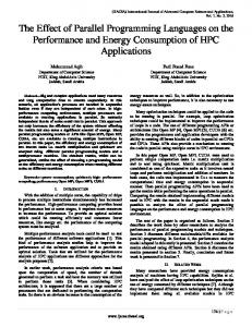
Figure 1.1: A program graph
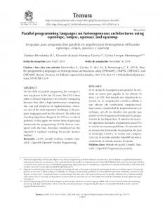
1.3.2 Parallel graph reduction Parallel graph reduction is the abstract execution mechanism which the functional language is presumed to use. A functional expression may be represented as a graph. For example consider the contrived expression bound to res: > res > > >
= x + y where x = 1 + 2 y = x + 3
The graphical representation of this is shown in Figure 1.1. The @ symbols represent function applications, left sub-graphs are functions and right sub-graphs are arguments. Notice how shared expressions are represented by shared graph nodes. Recursive expressions are represented by cyclic graphs. Evaluation proceeds by reducing graphs; for example + reduces both of its arguments to numbers, then the redex (node) is overwritten with the result of the addition, see Figure 1.2. Graph reduction is the process of locating redexes and reducing them by overwriting them with their values. Parallel graph reduction involves multiple tasks performing concurrent graph reduction. To prevent several tasks from reducing the same redex (node) a mutual exclusion mechanism is needed. This is achieved by tasks marking redexes. Thus in the previous example (Figure 1.1) the outermost + may reduce its arguments in parallel. (There is not much achieved by doing this here but it illustrates parallel graph reduction.) Therefore tasks will be created to evaluate the graphs corresponding to the arguments of + (x and y). The process of creating a task will be referred to as sparking. Each task will mark redexes it encounters to prevent other tasks from reducing them. Any task encountering a marked redex will block until the redex
CHAPTER 1. INTRODUCTION
7
Reduces to
@ @ +
3
2 1 Figure 1.2: A reduction @ @
@Y @
+
3
+ @X @ +
2 1
Figure 1.3: Concurrent reduction becomes unmarked; once unmarked the task will resume. Tasks unmark redexes (nodes) when they reduce (overwrite) them and they release any tasks blocked on that redex. In the example, the task evaluating y may block if the task evaluating x has not completed before it tries to access x. This is shown in Figure 1.3. Node marking has been shown by subscripting the appropriate node with X or Y to indicate which task is reducing which redex. Once the X task has evaluated x the @X node will be overwritten with 3 and unmarked; then the Y task can resume and perform its reduction. Now the deadlock question can be addressed. In parallel programming terms marking redexes corresponds to holding resources (mutual exclusion). Trying to evaluate redexes corresponds to demanding resources. Thus deadlock corresponds to a cycle of demands for redexes. However such a cycle is meaningless. It means that a value is dependent upon itself, for example: > a = a + 1
CHAPTER 1. INTRODUCTION
8
This equation has no solution; the value of a is dependent upon a and it is therefore unde ned. In a parallel interpreter this may give rise to deadlock, if the arguments to + are evaluated in parallel. A sequential implementation may loop inde nitely or some implementations may detect such self dependencies. Crucially, cyclic dependencies are the only way deadlock may arise. Thus deadlock can only arise in a parallel functional language for a program whose value is unde ned.
1.3.3 The advantages of parallel functional programming The advantages of parallel programming with functional languages are summarised below. These are in addition to the general advantages of functional programming, previously mentioned.
� Functional programs designed for parallel evaluation may be reasoned about in the same
way as sequential functional programs. � Parallel functional programs, unlike other parallel programs, need no communication, synchronisation or mutual exclusion to be speci ed explicitly. This all occurs implicitly in the program graph. � Deadlock can only arise when the result of a program is unde ned.
The determinacy of parallel functional programs means that all the techniques applicable to sequential functional programming are applicable to parallel functional programming. In particular parallel functional programs are amenable to transformation just as sequential functional programs are.
1.4 This thesis This section is a summary of the main results and contributions of this thesis. The basis of this work is a particular approach to parallel functional programming. This assumes an underlying machine model which is described in Chapter 2, along with various other proposed models. Essentially this is a shared memory MIMD machine: a generalisation of the locally available machine, GRIP [92]. The model uses a dynamic scheduling discipline; results by Eager give conditions necessary for good program performance, using such a scheduling discipline. The functional language used for expressing parallel algorithms is described in Chapter 3. It uses a parallel combinator for explicitly expressing parallel evaluation; it is argued that this is both necessary and desirable. Furthermore, it is argued that implicit detection of parallelism, via strictness analysis, in functional programs is extremely di�cult to do and indeed undesirable. The parallel functional language, and its assumed underlying machine model, are used throughout this thesis. Chapter 3 also discusses how di�erent parallel programming paradigms may be used with language. It is shown that several classes of algorithms may be expressed using the language, except for non-deterministic algorithms. To determine the e�ectiveness of example programs, written in the parallel language, a simulator was used. This is described in Chapter 4.
CHAPTER 1. INTRODUCTION
9
One of the nicest features of functional programs are their amenability to transformation. Squigol is an impressive algebraic style of program derivation and transformation. Chapter 5 investigates the suitability of Squigol for parallel program derivation; previously it has mainly been used for sequential algorithm derivation. It was discovered that some aspects of Squigol are speci cally orientated towards deriving sequential algorithms. However other aspects were found to be naturally suited to parallel algorithm derivation. This is discussed and it is demonstrated by three derivations of parallel algorithms: an all shortest paths graph algorithm, an n-queens algorithm and a greedy algorithm. Since the assumed machine is a shared memory one, task placement is unimportant; hence it is performed at run-time. However task size (granularity), the number of tasks in the machine and storage use are important issues. The target machine (an idealisation of GRIP) tries to control task granularity by using run-time heuristics. It is shown in Chapter 6 that to some extent this works; however for e�ective control this should be combined with various programmed techniques for controlling tasks granularity. As previously mentioned it is impossible to express non-deterministic algorithms in standard functional languages; even if their results are deterministic. Chapter 7 considers the introduction of bags (multisets) into functional languages. These admit a non-deterministic implementation but put an onus on the programmer to prove that they are used determinately. Usually such proofs are straightforward. Bags make some algorithms easier to write and more e�cient than would otherwise be possible. An implementation is sketched together with a proof that an intermediate implementation (a rewriting system) is correct. Chapter 8 considers the performance of parallel functional programs. It is shown by analysing some simple algorithms that writing e�cient parallel programs is more di�cult than it rst appears. For corroboration, the results of analyses are compared with simulation results. The analysis of algorithms which use pipelined parallelism is shown to be considerably more di�cult, and hence error prone, than analysis of other parallel algorithms. To this end, a formal semantics is developed for reasoning about pipelined parallelism. This may be used to generate recurrence relations and hence to analyse pipelined programs, as is demonstrated. The penultimate chapter (9) discusses further work. In particular some ideas on speculative parallelism, non-determinism, hybrid parallel and sequential algorithms and reasoning about parallel performance are discussed.
1.4.1 Thesis contributions The following contributions have been made by this thesis:
Parallel programming Contrary to some authors expectations I argue that parallelism should be explicitly expressed. In support of this I propose a simple parallel functional language. Extensive examples of parallel functional programs are given throughout this thesis. In particular the use of parallelism abstractions is expounded, especially divide and conquer ones.
CHAPTER 1. INTRODUCTION
10
Squigol A considerable amount of work exists on the Squigol methodology for program derivation. I develop and extend this work to parallel algorithms. In particular I demonstrate that homomorphisms are divide and conquer algorithms, that some Squigol optimisations are inherently sequential and I illustrate the use of parallel operators and rules via three example derivations.
Control of parallelism There have been many di�erent proposals in the literature for controlling parallelism. I show that for good control of parallelism (task numbers, storage use and task sizes) explicit control of parallelism is necessary, see Chapter 6. I propose various techniques for controlling data parallelism and divide and conquer parallelism. Experiments have been performed to measure the e�ectiveness of these techniques and to compare the best of them with a simple run-time heuristic for controlling parallelism.
Non-determinism Pure functional languages are insu�ciently expressive to implement many useful parallel algorithms. I have explained one way to extend a pure functional language: by adding nondeterministic bag structures, see Chapter 7. This proved e�ective; in particular bags enabled some algorithms proposed by Arvind [6] to be expressed which cannot be expressed in a pure functional language. The implementation of bags' non-determinism is di�cult; hence this was semi-formally developed via non-deterministic rewriting systems.
The performance of parallel programs The performance of parallel programs is nearly as important as their semantic correctness. There is a vast literature on the latter topic but very little on the former. I address the former in Chapter 8. I propose that to debug the performance of parallel programs di�erent levels of abstraction are required; this is demonstrated via several examples. In particular some programs are analysed at an abstract level and some others are simulated. To reason about programs performance at a very abstract level, analysis is required. There have been several proposals for analysing the performance of parallel strict programs. However such programs do not admit pipelined parallelism, an important form of evaluation. I have, therefore, developed a non-standard semantics for calculating the performance of pipelined programs.
Hybrid algorithms The goal of writing parallel programs for MIMD machines is not simply to obtain a program with maximal parallelism. In particular some parallel algorithms are not e�cient sequential ones. Thus, hybrid parallel and sequential algorithms are sometimes needed. The scan function analysed in Section 8.2.3, the greedy algorithm derived in Section 5.6 and the dc5 combinator used in Section 6.6 demonstrate this.
CHAPTER 1. INTRODUCTION
11
Non-determinism and proof obligations A general principle used to aid algorithm expression is the introduction of non-deterministic combinators into the language which may easily be proven deterministic. For example the par combinator of Section 3.1, the bhom function of Chapter 7, the choose function of Section 9.1.3 and the bb function of Section 9.1.1.
Chapter 2
Parallel machines This chapter surveys some parallel machines and discusses the parallelism issues which arise from them. In particular this chapter describes the machine to be used throughout the rest of this thesis. It is necessary to describe the target machine since any parallel programming language must be based on certain assumptions about the underlying machine. This is basically a generalisation of a locally-available multiprocessor: GRIP [92].
2.1 Parallel computer architecture The architecture of parallel computers was a `hot' research area a few years ago. Now its popularity has diminished as parallel machines are becoming commercially available. Nevertheless there are fundamental di�erences between the two major classes of parallel computer architecture. These classes are SIMD (Single Instruction stream, Multiple Data stream) and MIMD (Multiple Instruction stream, Multiple Data stream) architectures. The architectures have the same power and may simulate one another. However their di�erences mean that they are best suited to di�erent kinds of algorithm. Also they di�er in how parallelism must be organised for them to work e�ciently; thus di�erent approaches to programming them are needed. SIMD machines are array processors. They typically consist of a large collection of small processing elements. The same instruction is performed by all processing elements in synchrony. This means that the evaluation of programs on SIMD machines is usually deterministic, and hence programs may be reasoned about in the same way as sequential ones. SIMD machines are well suited to regular problems operating on large data sets. An example of a SIMD machine is the Connection Machine [46]. This was developed at MIT and it is intended to be programmed in Lisp. Hudak and Mohr have shown how graph reduction may be performed on SIMD machines by using a xed set of combinators [53]; however in practice this is very ine�cient. Also, O'Donnell has investigated the programming of SIMD machines using functional languages [85]. MIMD machines consist of cooperating processors each executing their own programs. These programs need not be the same and they are usually executed asynchronously. The nondeterministic evaluation of programs means that MIMD machines are harder to program than SIMD or sequential machines. However, as stated in the previous chapter, this is not true for functional languages. This thesis only considers MIMD implementations of functional lan12
CHAPTER 2. PARALLEL MACHINES
13
guages, of which there have been many proposals. MIMD machines may be sub-divided into two classes: shared memory (tightly coupled) machines and distributed (loosely coupled) machines. The essential di�erence between these two types of MIMD machines is that, memory access (communications cost) is constant for shared memory machines whereas for distributed machines the processor network topology a�ects memory access. Examples of shared memory functional language implementations are: ALICE, Buckwheat, Flagship, GRIP and the � -Gmachine [31, 38, 92, 63, 118]. Examples of distributed machines are Alfalfa, the HDG-machine the Nijmegen group's machine and ZAPP [38, 71, 111, 25]. For the purpose of this thesis the assumed target machine is a shared memory MIMD one. This thesis does not concern itself with any particular execution model for functional languages; other than the assumptions made about parallel graph reduction in Section 1.3.2. For more information on implementation details [88] is recommended.
2.2 Managing parallelism Managing parallelism is important in order to make a parallel program run e�ciently on an MIMD machine. Control may be e�ected by the program or via heuristics incorporated into the run-time system. The following issues have important e�ciency implications (for MIMD machines):
task and data placement: tasks and data should be arranged so as to minimise communica-
tion costs whilst maintaining parallelism. The placement of tasks and data should preserve task and data locality. The communication characteristics for shared memory machines mean that locality is less important than it is for distributed machines. scheduling: this is the task of assigning tasks to idle processors. If there are more tasks than idle processors, a choice must be made to determine which tasks to schedule (run) on the idle processors; this is almost always performed by the run-time system. The di�culty with scheduling is that di�erent schedules (orders of task execution) may result in di�erent execution times. task granularity and the number of tasks: these are related. Task overheads, such as communication costs, mean that there is a minimum size of task which is suitable for parallel evaluation. One measure of task size is the ratio of communications cost to execution cost. Also since tasks consume storage it is undesirable to generate many more tasks than there are processors. The rst two issues are described in this section, whilst the latter issue is investigated in Chapter 6, where several di�erent methods for programmer control of task granularity and the number of tasks are considered. Before describing strategies for task and data placement, and scheduling, two important types of parallelism are discussed.
CHAPTER 2. PARALLEL MACHINES
14
2.3 Conservative versus speculative parallelism Conservative parallelism is the term given to parallel evaluation where the results of all tasks are required. Conversely, speculative parallelism may produce tasks whose results are not required. Speculative parallelism is useful, and more general than conservative parallelism; however it is considerably harder to manage. In particular, parallel search algorithms often require speculative evaluation. Typically, a search space is concurrently searched until a desired element is found. Once the element has been found all other search tasks become redundant; however it is not known a priori which task will discover the element. Thus the parallel evaluation is speculative. For example to calculate in parallel the rst n prime numbers, using the sieve of Eratosthenes, many numbers are speculatively sieved in parallel. Another example is the n-queens problem. To calculate a single solution to this, in parallel, many di�erent partial solutions must be generated in parallel. Burton discusses speculative searching algorithms in [23]. The implementation di�culties of speculative parallelism arise because conservative tasks (those whose results are required) must be given priority over speculative tasks, or at least a fair scheduling discipline must be used. Otherwise the situation can arise where all a machines processors are evaluating speculative tasks, none of which terminate. Thus no progress will be made, although a result may exist. Further complications arise because speculative tasks may become conservative tasks or speculative tasks may need to be garbage collected (killed). In contrast the situation is far simpler if all parallelism is conservative because then any schedule will produce the same result from a program, if it exists. Hudak describes a sophisticated scheme to manage speculative parallelism [49]. It is a graphbased scheme which executes in a distributed fashion, concurrently with parallel graph reduction. However it has not been implemented and it appears to be quite complicated and costly. A similar scheme to Hudak's has been advocated by Partridge [87]. This manages speculative parallelism on a distributed machine. His scheme uses a storage garbage collector to collect garbage tasks. A priority system is used to ensure that normal order reduction is simulated and to ensure that the amount of redundant computation is minimised. Once again there is a lack of empirical evidence to support the scheme. An alternative and simpler approach has been proposed by many researchers, for example [43, 121]. This uses a notion of fuel; fuel corresponds to a quantity of evaluation which may be performed on a task, after which it is pre-empted. Some, known, conservative tasks may be given an in nite amount of fuel. This seems an interesting approach but again there is a lack of empirical evidence to support it. The implementation di�culties of speculative parallelism are so great that few functional language implementations support it. Therefore no programs are described in this thesis which require speculative parallelism, unless speci cally stated otherwise. Managing general speculative parallelism is not a problem which is speci c to functional languages (compare speculative parallelism with garbage collection for instance).
CHAPTER 2. PARALLEL MACHINES
15
2.4 Distributed machines: task and data placement The dominant parallelism management issues for distributed machines are task and data placement. Although such machines are not the subject of this thesis, several interesting ideas, which have been proposed, are discussed in this section.
2.4.1 ZAPP The ZAPP project focussed on divide and conquer algorithms [25]. This restriction meant that a run-time heuristic was su�cient to e�ectively control task and data placement. Initially a program was loaded onto a single processor. Tasks were produced and these were subsequently stolen by neighbouring processors. Thus tasks di�used from the original root processor. This ensured a reasonable degree of locality for divide and conquer algorithms' tasks.
2.4.2 Sarkar's system Sarkar [100] has investigated the automatic partitioning and scheduling of programs at compiletime. This was performed with SISAL programs from which static networks of tasks were extracted. Thus, the programmer has no control over locality or granularity. SISAL is a rst order single assignment language. The actual partitioning and scheduling is performed on GR, a graphical representation of SISAL or any other rst order language. GR does not express a program's semantics, instead it contains estimates of a program's performance characteristics. These estimates include the program's parallelism, execution time, communications costs and synchronisation points. GR is limited in the kind of parallelism it can express since it is intended for compile-time analysis. Complementing GR is a performance model of the target machine. This contains information on processor execution times, scheduling and communications overheads. Algorithms are used for partitioning (splitting a program into tasks) and scheduling at compile-time. These algorithms try to optimise the mapping of a GR program representation onto particular machine model. Sarkar's system performs well for static programs where computation does not vary much for di�erent inputs. It is unsuitable for programs whose computation is very input dependent. Since static analysis of higher order languages is much harder than for rst order languages; it is also unsuitable for these.
2.4.3 Caliban Paul Kelly has proposed an extension to Miranda to support the explicit mapping of tasks to processors, called Caliban [70]. The programmer speci es a static network of tasks which are mapped onto a distributed machine, rather like occam [75]. In Caliban, function de nitions may be augmented with clauses specifying task placements, where tasks correspond to functions. Networks of stream-processing functions may be constructed which are statically mapped onto a loosely-coupled architecture. These connection speci cations are written in a functional style; however a formal semantics for them has yet to be de ned. Thus task sizes and task locality are completely determined by the programmer.
CHAPTER 2. PARALLEL MACHINES
16
2.4.4 Para-functional programming Para-functional programming has been devised by Hudak [54]. Essentially, a dynamic network of tasks is speci ed by the programmer. This is dynamically mapped onto a computer's architecture at run-time. Annotations in a program are used to specify that certain expressions constitute tasks and that they should be evaluated in parallel. They also are used to specify particular processors on which expressions (tasks) should be evaluated. This processor addressing may be absolute or relative, for example: exp $on left($self) means that exp should be evaluated on the processor to the left of the current processor. A semantics for Hudak's para-functional language is described in [51] (the original semantics as given in [54] is erroneous). Just as with Caliban, locality and task granularity is completely determined by the programmer. This strategy encompasses all programs which can be written in Caliban. It is well suited to problems with a regular structure. However for problems with an irregular task distribution, an adaptive run-time heuristic may be better. For example it is di�cult to e�ciently map an irregular tree of tasks (unknown at compile-time) onto an architecture, using explicit task placement instructions. This scheme has not yet been implemented and there are many remaining questions; for example what happens if multiple tasks are mapped onto the same processor?
2.4.5 Concurrent CLEAN The Nijmegen group are investigating the distributed implementation of a functional language, based on graph rewriting [111]. The intermediate language they use, Concurrent CLEAN, has annotations to denote sequential and parallel evaluation. The novel part of their approach is language annotations to control graph copying. When a task is created, its graph must be copied onto another processor. Copying is the norm and annotations determine how much graph should be copied by preventing the copying of graph they annotate. As a general rule only graph in WHNF should be copied. These annotations do not strictly prevent copying, rather they defer copying until the graph becomes evaluated. Once evaluated, graph whose copying has been deferred, is copied. These annotations allow the creation of arbitrary process network topologies and they support synchronous and asynchronous process communication. They claim that such copying control is necessary for e�cient distributed implementation.
2.5 Shared memory machines: GRIP GRIP is a shared memory MIMD machine [92]. As previously mentioned task and data placement on shared memory machines are not as important as on distributed machines. Thus task and data placement on shared memory machines, such as GRIP, are usually performed by run-time heuristics. An important feature of GRIP is that it uses an evaluate-and-die task model [91]. This means that sparking an expression does not reserve the expression for evaluation by the new task; the expression will be evaluated by the rst task requiring its value. This mechanism tends to coalesce tasks and hence it can increase the granularity of parallelism. This is discussed further in Section 6.3.1.
CHAPTER 2. PARALLEL MACHINES
17
In addition GRIP discards sparks once it becomes loaded beyond a certain limit; this prevents the machine from becoming ooded with tasks.
2.6 Scheduling: Eager's result For run-time scheduling to work well a program's performance must not be too dependent upon scheduling. This section describes some work which determines conditions under which this holds. Eager et al. [36] have analysed the performance of parallel programs running on a machine with run-time scheduling. Their results are quite abstract; they provide bounds on the performance of a parallel program using only a few simple measures. Some terms are now de ned. Speedup is de ned to be the ratio of sequential execution time to parallel execution time for a program run on an n-processor machine. Thus the best possible speedup for a program run on an n-processor machine is n (linear speedup). The measure used to characterise parallel programs is their average parallelism; this has several equivalent de nitions, including: the speedup given an unbounded number of processors, and the average number of processors that are busy during the execution of a parallel program, with an unbounded number of processors available. The former measure is used in some performance analyses in Chapter 8. The latter measure is used in the experimental simulator, Chapter 4. The following result has been used a great deal in this thesis:
2.6.1 Eager's speedup theorem Let A be the average parallelism of a program and let S (n) be the speedup with n processors. Then for any work-conserving scheduling discipline:
n�A S (n) � n + A?1 A work-conserving scheduling discipline is one that never leaves idle a task that is eligible for execution when there is a processor available. The assumed target machine does have a workconserving scheduling discipline; however GRIP does not, since it may discard sparks (tasks). A simple corollary of this is that if A�n then a good speedup will result. Thus a program is well suited to run on an n-processor machine with run-time scheduling if A�n. If it is not the case that A�n then scheduling becomes much more important and an explicit scheduling discipline is desirable. In general explicit scheduling is not practical, except in the extreme case when no scheduling needs to be performed. That is, when a static network of tasks are statically mapped one-to-one onto a machine's processors. When this occurs the following usually holds: A � n. However as previously mentioned the subject of this thesis is mainly MIMD machines with run-time scheduling; therefore it is required that A�n. Notice that to obtain a good speed-up there must be many more tasks than processors. This contends with the parallelism management issue of not swamping the machine with tasks.
CHAPTER 2. PARALLEL MACHINES
18
2.7 The target machine The assumed target machine for all programs in this thesis is a MIMD shared memory one, an idealisation of GRIP [92]. It is assumed that task and data placement are performed by the machine's run-time system. Thus no task or data placement information is speci ed by programs. Most importantly it is assumed that an evaluate-and-die task model is used; however unlike GRIP no sparks are discarded. Therefore all that programs need to specify is: what to spark ? Throughout this thesis, unless otherwise stated, this will be the target machine. However, remarks will also be made on the implications of discarding sparks, like GRIP does.
Chapter 3
Parallel functional programming This chapter describes a particular approach to parallel functional programming. Any parallel programming language must be based on certain assumptions about the underlying machine. The intended target machine for programs in this thesis is described in the previous chapter. The philosophy behind my approach to parallel programming with functional languages has been to nd the minimum necessary to write e�cient parallel functional programs for the target machine. In particular it was desired to relieve the programmer from as much parallelism organisation as possible, whilst not relying on any as yet unproven compile-time analyses. The underlying assumptions of my approach to parallel functional programming may be summarised thus:
� The programmer must devise a parallel program and annotate it to indicate which expres-
sions are suitable for parallel evaluation. � The target machine is assumed to be an MIMD one with a shared memory. Task and data placement are performed by its run-time system. Thus the programmer is responsible for addressing the question what to spark ? but not where or when to execute tasks. � No automatic partitioning, scheduling, parallelisation or task placement is performed by the compiler. Rather the programmer and run-time system are responsible for performing these tasks.
It is argued that automatic detection of parallelism using strictness analysis is not su�cient alone to produce e�cient parallel programs. Furthermore it is argued that the explicit expression of parallelism is in any case very desirable. After describing the parallel functional language and arguing for the explicit expression of parallelism, parallel algorithms and programming paradigms are discussed. It is shown that functional languages are well suited to implementing some algorithms but not others. In particular functional languages cannot express non-deterministic algorithms.
19
CHAPTER 3. PARALLEL FUNCTIONAL PROGRAMMING
20
3.1 A parallel functional language This section describes how the functional language is extended so it can express parallel algorithms. To achieve this a parallel and sequential combinator are used. The semantics and operational behaviour of these combinators are discussed. Lastly, an algebraic technique for removing some redundant sparks is presented.
3.1.1 A parallel combinator It is necessary to express in programs what to spark. New syntax, such as annotations, could be added to the language, but for simplicity and economy of concepts a parallel combinator (par) is used: > par :: * -> ** -> * par a b = b
Informally, par sparks its rst argument and returns its second argument. It is the only source of parallelism in the language. Tasks are only evaluated to WHNF; greater evaluation may be achieved by using multiple pars to evaluate the components of data structures. A bene t of having a parallel combinator is that no changes to the front end of a compiler are necessary, since par may be treated as a function syntactically and semantically. (An alternative method for expressing parallelism, due to Burn, is described in Section 3.2.3.) A typical parallel expression might have the form: (par e1 . par e2 . � � � . par en) exp. The meaning and evaluation of the expression have been separated: the meaning is exp and all the expressions e1 through to en are sparked. Other combinators could have been chosen, for example a parallel apply combinator; however par was found to be the easiest to use. What should the semantics and operational behaviour of par be? There are several alternatives: 1. The par combinator could be strict in its rst argument: par ? x = ?. Operationally par x y sparks x and then evaluates y. The application par x y is only overwritten with the value of y when x has completed. This is necessary to ensure strictness. The problem with this behaviour is that it is overly-synchronous and it does not permit pipelined parallelism. For pipelined parallelism with lists, an expression like par h (par t (h:t)) is required to return the cons value before the evaluation of h and t have completed. This cannot happen with this particular version of par. 2. The par combinator could be non-strict in its rst argument: par ? x = x. Operationally par x y must spark x and then return y. However since x may not terminate, parallelism may be speculative. As previously mentioned speculative parallelism is very general but very di�cult to implement, see Section 2.3. 3. The meaning of par could be non-deterministic; that is par ? x may be ? or x. This behaviour arises from most practical implementations of par because scheduling is not usually fair. In such cases, if x blocks then it is possible for non-terminating tasks to prevent x from ever being resumed, especially if ? creates many non-terminating tasks.
CHAPTER 3. PARALLEL FUNCTIONAL PROGRAMMING
21
The second option is chosen for the meaning of par, that is par x y = y. However par will be implemented non-deterministically, as per the third option. This implementation of par is not generally valid for all uses of par, but it does mean that par may be e�ciently implemented, and it will not needlessly constrain parallelism. Two operationally di�erent pars are discussed, both of which behave non-deterministically. It is assumed that unless otherwise stated all programs and results in this thesis use a par which always sparks its rst argument. In addition the GRIP implementation of par, which may or may not spark its rst argument is discussed. When the GRIP implementation of par is discussed it will be referred to by phrases such as \if a GRIP-like spark discarding strategy is used". In order for the non-deterministic implementations of par to respect the semantics of par, the way in which par is used must be constrained. In particular it must be ensured that the rst argument of par is de ned, unless the result, the second argument, is unde ned. This par constraint may be formulated thus: For all applications of par
x y,
the following must hold: x = ? ) y = ?.
The latter condition is just a reformulation of strictness; this is explained in Section 3.2.1. This represents a constraint on how par may be used. If this constraint is met then the nondeterministic implementations of par will respect par's semantics. The constraint on how par may be used can either be a proof obligation for programmers using par, or it can be veri ed mechanically using, for example, a strictness analysis (see Section 3.2.1). Alternatively if pars are automatically placed then this constraint must always be met. For example the pars in the following two programs do not satisfy the constraint: > funny1 >
= f 0 where f n = par (f (n+1)) n
In order for funny1 to be a valid program the par in it must satisfy the constraint. However the expression f (n+1) does not satisfy the par constraint. Thus the par in funny1 does not satisfy the constraint and hence funny1 is not a valid program. > funny2
= par (error "FAIL") "OK"
The error function is similar to bottom: it causes the program to be aborted, and its rst argument to be output. Thus since "OK" de nitely terminates, this par also does not satisfy the constraint. In [40] it was recognised that two forms of parallelism annotation are required: one for function de nitions and one for function applications. These may both be expressed using par. For example a function f x = exp which should spark its argument may be written: > f x
= par x exp
CHAPTER 3. PARALLEL FUNCTIONAL PROGRAMMING An application app > app >
= g exp
22
whose argument exp should be sparked may be written:
= par e (g e) where e = exp
In both cases the par constraint must be satis ed.
3.1.2 A sequential combinator In addition to par a sequential combinator, seq, is needed. The seq combinator is strict in both arguments; operationally, it evaluates its rst argument to WHNF, then discards it and returns its second argument. > seq :: * -> ** -> ** seq x y = y, if x =
6 ? = ?, if x = ?
At rst it seems curious that a sequential combinator is needed for expressing parallel evaluation. There are three reasons for needing seq. Firstly for strict operators whose order of argument evaluation must be changed. For example (assuming left to right argument evaluation) consider:
: : : par
x (if cond then seq y (x+y) else seq z (x-z))
:::
The un-sparked variables in the arithmetic expressions must be evaluated before trying to evaluate the sparked variables. Otherwise evaluation might block on the sparked variables and parallelism will be lost. If the evaluation order of strict operators is speci ed then some, but not all, seq combinators may be removed; for example with left to right evaluation, the example above may be rewritten:
: : : par
x (if cond then y+x else seq z (x-z))
:::
Secondly, seq may be used for evaluating data structures `further' than WHNF. The par combinator can be used in place of seq but sometimes this is not desirable because the tasks produced are too small to be useful. For example a parallel map for binary trees: > bintree * > > treemap f (Leaf x) > treemap f (Node l r) > > >
::= Node (bintree *) (bintree *) | Leaf * = seq res (Leaf res) where res = f x = par ml (par mr (Node ml mr)) where ml = treemap f l mr = treemap f r
CHAPTER 3. PARALLEL FUNCTIONAL PROGRAMMING
23
The seq ensures that the application f x is performed before it is required (demanded). If the seq was omitted evaluation of treemap would stop at Leafs. The seq could be changed to a par; this might improve performance by allowing pipelined parallelism to occur. However it could also be detrimental, since it could create many small tasks. Depending upon the context in which treemap was used it might not be necessary to spark both ml and mr. Thirdly, sometimes it is desirable to guarantee evaluation. This can be useful for a GRIP-style system where pars may not spark their rst arguments. For example consider the treemap function above, a likely behaviour for GRIP is this: initially GRIP will not discard sparks, then once it becomes loaded with tasks, it will discard sparks. When sparks are discarded then the results of previously sparked tasks will be (Node ml mr) where ml and mr are unevaluated closures. It would be far better for ml and mr to be evaluated albeit sequentially. This can be achieved by using a new form of par, de ned using par and seq, newpar: > newpar x y
= par y (seq x y)
The newpar combinator is strict in both arguments. It has the advantage over par that there is no constraint on how it may be used. This is because the par in newpar always satis es the par constraint because the rst argument to par, y, is always evaluated by seq. The treemap function may be rewritten: > treemap f (Leaf x) > treemap f (Node l r) > > >
= seq res (Leaf res) where res = f x = newpar ml (newpar mr (Node ml mr)) where ml = treemap f l mr = treemap f r
The problem with using newpar, or putting seqs directly into treemap, is that pipelined parallelism is prevented. Each Node constructor is not built until both ml and mr have been evaluated. Thus, none of the result of treemap will be returned until the whole result has been evaluated. For this reason newpar is not used. In Section 9.1 this and some other drawbacks of using par and seq combinators to explicitly express parallelism are discussed. The seq combinator is not a new idea. It has been used in sequential functional languages for controlling evaluation order, for example to control functions' input and output behaviour.
3.1.3 Removing redundant parallelism Sometimes it is possible to remove redundant sparks, which may have been inadvertently inserted into programs. This may be performed by using algebraic reasoning, which ensures only redundant pars are removed. As an example consider Quicksort: > qsort [] = [] > qsort (e:r) = (par qlo . par qhi) (qlo ++ (e:qhi)) > where
CHAPTER 3. PARALLEL FUNCTIONAL PROGRAMMING > >
24
qlo = qsort [x| x qsort (e:r) = par qhi (qlo ++ (e:qhi)) > where > qlo = qsort [x| x qsort :: [num] -> [num] > qsort [] = [] > qsort (e:r) = qsort (fillo r) ++ (e:qsort (filhi r)) > where > fillo = filter ( filhi = filter (>=e)
This function will be used as an example to show the information given by strictness analysis. For simplicity only the top level expression of the second equation will be analysed, which consists of monotyped rst order function applications. The following contexts will be used to describe strictness: L and S will represent lazy and strict contexts for integers. A lazy context means that an expression may or may not be evaluated to WHNF. A strict context is one in which an integer expression will be evaluated to WHNF. For lists of integers, the contexts HT, T, S, and L will represent: head and tail strict, tail (spine) strict, strict (to WHNF) and lazy, respectively. Below are tables representing how contexts may be propagated. These tables show the degree to which a function's arguments may be evaluated, given that the function application occurs in a certain context.
CHAPTER 3. PARALLEL FUNCTIONAL PROGRAMMING qsort
context L S T HT
arg1 L HT HT HT
fillo/filhi context arg1 L L S S HT T HT HT
context L S T HT
++
arg1 L S T HT
arg2 L L T HT
28 context L S T HT
:
arg1 L L L S
arg2 L L T HT
For example in a tail strict context (T) an application of fillo will be head and tail strict (HT) in its argument. Assuming that an application of qsort occurs in at least a strict context (L), the top level applications of the second qsort equation can be labelled thus: @HT (@HT
++
(@HT
qsort
(@HT
fillo r)))
(@HT (@S
: e)
(@HT
qsort
(@HT
filhi r)))
Notice how small the original expression is and how many annotations have been generated (the lter functions have not been shown!). Worse still, in general functions will have many di�erent annotations according to the context in which they occur. Thus many function versions may be required. The problem with these annotations is that many of them are redundant with regards to parallelism, and di�erent operational interpretations may be given to them. The annotations could be interpreted as indicating the amount of parallel evaluation possible; for example HT could mean that all a lists elements may be evaluated in parallel. Equally, annotations could be interpreted as meaning the amount of sequential evaluation possible (call by value evaluation). For example the parallel interpretations of @HT and @S are shown below: @HT f l = ht f l @S f x = s f x > ht f l > > >
= par (p l) (f l) where p [] = () p (x:xs) = par x (p xs)
> s f a
= par a (f a)
Thus the qsort expression could be validly transformed to: ht (ht (++) (ht qsort (ht fillo r))) (ht (s (:) e) (ht qsort (ht filhi r)))
However this expression generates many redundant tasks; that is many tasks are generated which do little or no evaluation. Producing redundant tasks may greatly impede a machine. Tasks consume storage and they require communication resources if evaluated on another processor. A GRIP-like machine which employs dynamic control of task numbers, will discard tasks once it becomes heavily loaded. If a machine becomes loaded with redundant tasks crucial parallel tasks may be discarded. A more operationally e�cient transformation would be:
CHAPTER 3. PARALLEL FUNCTIONAL PROGRAMMING
29
s ((++) (qsort (fillo r))) ((ss (:) e) (qsort (filhi r)))
Where: > ss f a
= seq a (f a)
This does not generate redundant tasks, although it still does generate some very small tasks for example qsort []. This problem is discussed further in Chapter 6. Producing too many tasks and producing too small tasks is a real problem, for example see [39]. This demonstrates that transforming an expression into an operationally e�cient parallel one requires much more than just strictness information. Either additional complex analyses or manual help are required. As a further example consider the lter expressions in qsort; since lter is used in a head and tail strict context (HT), these lterings could be performed in parallel: > parfilter :: (*->bool) > parfilter p [] = > parfilter p (x:xs) = > > > >
-> [*] -> [*] [] par rest l where l = x:rest, = rest, rest = parfilter p xs
p x otherwise
However, for most MIMD machines this granularity of parallelism (the size of tasks which are produced) will be too small. The tasks which are produced will not be worth evaluating in parallel. Nevertheless they will consume storage and communication resources, and for a GRIP-like machine which discards tasks, they may prevent other more worthy tasks from being evaluated.
3.2.3 Evaluation transformers Burn has proposed evaluation transformers to solve some of the problems with using strictness analysis to determine parallelism [18, 19, 20, 71]. Evaluation transformers solve the problem that di�erent amounts of evaluation may be possible in di�erent contexts. For example in the context of sum exp all the elements of the list exp may be evaluated in parallel. In the context of # exp only the spine of the list may be safely evaluated; this yields no parallelism and hence should be done sequentially. For a rst order language the di�erent contexts in which expressions occur may be statically determined. However for a higher order language, the contexts in which expressions occur may be data dependent and hence not statically determinable. For example consider the apply function: > apply f a
= f a
The context in which the second argument to apply occurs, that is the amount of evaluation which may be performed on the second argument, depends on the rst argument. In general this can only be determined dynamically; if this is not done parallelism may be lost.
CHAPTER 3. PARALLEL FUNCTIONAL PROGRAMMING
30
Evaluation transformers propagate evaluators. Evaluators are similar to the strictness contexts and parallel functions (ht and s) of the previous section. Evaluators and rules for propagating (transforming) them are derived by an abstract interpretation. Some evaluators may be statically determinable, whilst others may need to be dynamically determined at run-time. Propagating evaluators dynamically at run-time gives more information and hence potentially more parallelism than only utilising statically determinable evaluators. However there is an implementation overhead associated with propagating evaluators at run-time. Only utilising statically determinable evaluators yields less information and hence potentially less parallelism than propagating them at run-time. However there is no implementation overhead associated with static evaluators. In addition, if evaluators are propagated at run-time and program graph nodes are marked with evaluators, some re-sparking may be prevented. A similar e�ect to evaluation transformers may be achieved by just using par and seq. Functions may be given an extra parameter which corresponds to an evaluator. These evaluator arguments can be passed between functions and transformed as necessary. For example the papply function below is parameterised so that in di�erent contexts it may evaluate its second argument to di�erent degrees: > papply f e a
= par (e a) (f a)
> pl [] > pl (x:xs)
= () = par x (pl xs)
Thus if apply was applied to a hyper-strict function on lists of integers, f, the following apply function could be used: papply f pl exp. This would evaluate all the elements of the list exp in parallel. It seems di�cult to implement evaluation transformers, in their full generality, using this method. If evaluation contexts were expressed in this way then those such as papply f pl exp which are statically determinable, could be specialised using partial evaluation. This would remove the need, in some expressions, to propagate evaluators, just as occurs with Burn's statically determinable evaluation contexts. The prevention of re-sparking cannot be e�ciently achieved using par and seq since this requires graph nodes to be marked with evaluators. These node markings must be updated when a node is evaluated by an evaluator. However it may be possible to achieve this e�ect at compile time by performing some manipulation of expressions; see for example Section 3.1.3, where an algebraic method for removing some redundant pars is presented. Evaluation transformers are unproven. It is unclear whether evaluators are capable of capturing enough forms of parallel evaluation, especially for di�erent data structures, to be useful. In order to use evaluation transformers in their full generality an implementation such as described by Burn in [19] is probably necessary. However for a more limited use of evaluation transformers seq and par may be su�cient. If evaluation transformers are incorporated into a run-time system, then they can prevent some re-sparking, which could not be prevented by using just par and seq. However, neither evaluation transformers nor par and seq can prevent the creation of all small tasks. Evaluation transformers were originally designed to be used with programs containing implicit parallelism. It maybe possible to use evaluators for explicitly expressing parallelism in a similar way to par and seq. However this thesis investigates how well a simpler approach works.
CHAPTER 3. PARALLEL FUNCTIONAL PROGRAMMING
31
3.3 Explicit expression of parallelism The previous section has argued that just using strictness analysis to determine the parallelism in programs, is unlikely to produce e�cient parallel programs. This section argues that it is in any case positively desirable to express parallelism explicitly. In the context of the parallel functional language previously presented, the explicit expression of parallelism means that pars and seqs should be inserted into programs by the programmer. The onus is on the programmer to prove that applications of par satisfy the par constraint (the par proof obligation). Notice that by requiring parallelism to be expressed explicitly the original advantages of using functional languages generally, and speci cally for programming parallel computers, have been retained: there is still no need to specify communications, and deadlock is not a problem. Burton, Hudak and the Nijmegen group have also proposed explicit parallelism expression [22, 54, 111]. However their main aim was to program distributed machines and thus to address locality issues, rather than what to spark, which this thesis addresses. Hughes has also suggested explicit concurrency; however his main aim was to reduce the space usage of functional programs [58]. His || combinator is an in x version of the par combinator used here.
3.3.1 A scenario There are are compelling reasons to believe that explicit parallelism expression is desirable. Programming in all its forms, from conventional programming through to sophisticated program derivation, consists of re ning a high level problem speci cation (possibly in the programmers head) to an executable algorithm. The parallel programmer must ultimately produce a parallel program and this is, not surprisingly, a major consideration in the programs design. Without explicit parallelism expression one can imagine the following programming scenario: a programmer designs a parallel functional program for a parallel machine. Throughout the algorithms development, parallelism has been uppermost in the programmers mind. The resulting program is fed into a compiler. The compiler then carefully analyses the program to re-discover the programmers parallelism. It is evident from this that the programmer should know where the parallelism is in their program but cannot communicate this to the compiler. Most likely the programmer will comment various parts of the program with their intentions like \evaluate elements of the list xyz in parallel". Unfortunately the programmer can but hope that the compiler will discover this parallelism. Of course a compiler may discover more parallelism than a programmer intended, but this is sheer luck and I do not believe in programming by luck! When writing parallel programs, parallel evaluation is not just a desirable optimisation that a compiler may discover; it is a fundamental property of programs.
3.3.2 Parallelism declaration Lack of parallelism documentation or lack of explicit parallelism expression could result in a programmer (or compiler) unwittingly removing parallelism. This may arise because often much more e�ciency is achievable with a sequential algorithm on a sequential machine
CHAPTER 3. PARALLEL FUNCTIONAL PROGRAMMING
32
than with a parallel algorithm on a sequential machine. For example for accumulate (also known as scan or parallel pre x), an algorithm exists which on a parallel machine with n processors has O(ln n) time complexity. The same algorithm if run sequentially has has complexity O(n ln n). However a simple O(n) purely sequential algorithm does exist. Thus, a programmer or a compiler might inadvertently transform the parallel algorithm to the sequential algorithm. This would result in a much more sequentially e�cient algorithm at the expense of removing all parallelism. The performance of accumulate is discussed further in Section 8.2.3. This destroys the idea that a computer may be regarded as a black box which a programmer knows nothing about. The programmer and compiler must both know what is in the box, at least whether it is a parallel or sequential machine, and the program must express this too. Another example illustrating this point is sorting. On a sequential machine the two main issues in choosing a sorting algorithm are the input size and its distribution (how sorted the input is likely to be). For a parallel machine these are important too, but also the number of processors compared to the input size is important. If the number of processors is large then a parallel sort like bitonic merge sort (see for example [93]) may be appropriate. However, each individual processor should execute a more e�cient sequential sorting algorithm since bitonic merge sort is not an e�cient sequential algorithm. The parallel algorithm should be used to distribute work across processors, each of which does e�cient sequential sorting. Again this is discussed further in Section 8.2.3. A further point supporting the case for explicit parallelism expression is related to a more general functional language problem. When functional languages are said to be `declarative' what is really meant is that they are declarative in meaning; that is programs declare the values which they compute. One could argue that imperative languages are declarative too. They are declarative operationally, because they declare how to compute values (not what the values are). There have been two approaches to functional languages' lack of operational speci cation, which leads to ine�cient implementation and makes reasoning about their operation di�cult. The rst approach is to develop analyses to extract the required operational information automatically, for example strictness analysis and in-place-update analysis. The second approach is to augment functional languages with explicit operational information. One horrible extreme of this is having assignment, like in ML. The other extreme are extensions to functional languages which do not compromise them: for example Wadler's linear type system [116]. The parallelism extensions I propose, par and seq, do not unduly compromise functional languages.
3.4 Algorithm classes and programming paradigms This section describes parallel algorithm classes and parallel programming paradigms. In particular the suitability of the parallel functional language to these classes and algorithms, is discussed. Quinn's classi cation of algorithms is explained and the di�culty of expressing certain algorithms is highlighted. The last two sections discus two parallel programming paradigms; both are suited to parallel functional programming.
CHAPTER 3. PARALLEL FUNCTIONAL PROGRAMMING
33
3.4.1 Quinn's algorithm classi cation Quinn in his book [93] describes a useful classi cation of parallel algorithms for MIMD machines:
partitioned: these algorithms divide a problem up into sub-problems which are solved in par-
allel. All sub-problems are solved using the same procedure. The sub-problem solutions are combined to form the problem solution; divide and conquer algorithms are typical partitioned algorithms. In general partitioned algorithms are very synchronous and hence they are sometimes termed synchronous algorithms. pipelined: these algorithms consist of a sequence of tasks, each of which solves a di�erent problem. The task are connected so that the output of one task feeds the input of another task. This type of parallel algorithm gives an increased throughput over a sequential algorithm. An example of a pipelined algorithm is a parallel compiler where all the phases are performed in parallel: lexing, parsing, code generation and code optimisation are all separate tasks. Synchronisation in a pipelined algorithm is implicit and arises between producers and consumers of data. relaxation: these algorithms are also termed asynchronous or non-deterministic algorithms. They are characterised by being able to work with the most recently available data. Thus task synchronisation is minimised. Relaxation algorithms may be similar to partitioned or pipelined algorithms; the key point is their ability to work with di�erent amounts of information about the problem being solved. Many relaxation algorithms require some form of speculative parallelism. An example of a relaxation algorithm is the parallel union- nd algorithm, described in [93]; this may be used to solve many graph problems. Ban^atre et al. have a discipline of programming based on relaxation algorithms [8]. These are speci ed as non-deterministic rewriting systems. Often algorithms contain parts from di�erent classes of parallel algorithms. For example, the top level an algorithm may be expressed as a pipelined algorithm; however, individual tasks in the pipeline may be partitioned algorithms. A signal processing algorithm may typically have this structure. Any functional language may naturally express partitioned parallel algorithms, such as divide and conquer algorithms. For example a function for summing the leaves of a binary tree (treesum) may be written thus: > bintree * >
::= Node (bintree *) (bintree *) | Leaf *
> treereduce f (Leaf x) > treereduce f (Node l r) > > >
= x = par ll (par rr (f ll rr)) where ll = treereduce f l rr = treereduce f r
> treesum
= treereduce (+)
CHAPTER 3. PARALLEL FUNCTIONAL PROGRAMMING
34
The proof obligation associated with par means that treereduce is valid program if f is strict in both arguments or if f is total and the input tree is completely de ned. To express pipelined algorithms a functional language must have non-strict data structures, for example streams. (This is a rarely-mentioned advantage of lazy languages over strict ones.) Pipelined algorithms rely on evaluation with only partial information. A consumer task (function) must be able to do some evaluation with only partial information (for example part of a list) produced by some producer task. The sieve of Eratosthenes for generating all the prime numbers less than one thousand is an example of a pipelined algorithm: > primes > >
= par (forcespine sp) sp where sp = sieve [2..1000]
> sieve [] > sieve (p:nos) > > >
= [] = par (forcespine filtnos) (p:sieve filtnos) where filtnos = filter pred nos pred n = n mod p ~= 0
> forcespine [] = [] > forcespine (x:xs) = forcespine xs
Since sp in primes is completely de ned, the par in primes satis es the par constraint. The sieve function occurs in at least a tail strict context, hence the par in sieve also satis es the par constraint. This program uses sieve to successively lter multiples of prime numbers from a list of the rst thousand numbers. Each prime number ltering is performed in parallel. Thus consecutive sieve operations form a pipeline. The program is expressed so that it may form part of a pipeline; primes become available as they are generated. Notice how forcespine is used to force each ltering; this is required because par only evaluates its rst argument to WHNF. This is another example of where sequential evaluation is needed in a parallel program. (A parallel lter would have produced too small tasks.) This algorithm is quite complex; often pipelined algorithms are more complex than partitioned ones. A simulator/debugger is useful for debugging the performance of such algorithms (see Section 8.6). Relaxation algorithms are inherently problematical for functional languages due to their nondeterminism. Functional languages are inherently deterministic because expressions denote unique values. The theoretical implications to programming language semantics of nondeterminism have been widely studied, for example [102]. Some interesting practical solutions to the problem have been proposed by: Burton (improving values), John Hughes (sets) and LeM�etayer (gamma model). Chapter 7 discusses these proposals and a limited form of nondeterministic construct is proposed for functional languages. Section 9.1.1 also discusses some more ideas concerning non-determinism. The implementation di�culty of algorithm classes correlates with their amount of synchronisation. Partitioned algorithms are easy to implement in any language; pipelined algorithms are a
CHAPTER 3. PARALLEL FUNCTIONAL PROGRAMMING
35
little harder to implement. Relaxation algorithms, assuming they can be expressed, are hard to implement; in particular detection of termination can be non-trivial, see Section 7.6.2 and [8]. Also in correlation with the synchronisation of the various algorithm classes, is the di�culty of reasoning about algorithms performance. The performance of partitioned algorithms is relatively easy to reason about. Pipelined algorithms are harder to reason about. In Section 8.3 a semantics to formalise reasoning about pipelined parallelism is presented. The performance of relaxation algorithms is notoriously hard to reason about; often this is because the performance of relaxation algorithms is unpredicatable!
3.4.2 Carriero and Gelernter's paradigm Carriero and Gelernter in [26] present three parallel programming methods based on three conceptual classes of parallelism. These classes of parallelism roughly correspond to the three classes of algorithm previously described. The conceptual classes are:
result parallelism: with this class of parallelism each task produces one piece of the result.
This corresponds closely to the class of partitioned algorithms. specialist parallelism: here each task performs one speci c kind of activity. This corresponds closely to the class of pipelined algorithms. agenda parallelism: a global agenda is kept and each task performs an operation according to the current agenda. This paradigm has similarities with the relaxation class of algorithms. With each of the above conceptual classes of parallelism there are three associated parallel programming methods:
live data structures: here data structures are transformed by tasks into a result data structure.
message passing: this style involves the splitting of a problem into its logical parts; resulting
tasks communicate using message passing. Thus tasks are specialised. distributed data structures: this lies between the extremes of live data structures and message passing. A group of data objects and tasks exist. Tasks can perform many activities on data objects. Tasks actively look for data objects on which to perform a given activity. Data objects may be shared, which is how tasks communicate. To explain these three methods of parallel programming, an example is used (taken from [26]). Consider a naive n-body simulator. On each iteration of the simulation, forces between all objects are calculated and the new object positions are determined. The live data structure solution to the problem consists of a matrix representing objects and their positions. A function to calculate a new matrix of positions is de ned. This function implicitly creates tasks to determine the new position of each object from the old matrix of object positions. The message passing approach entails simulating each object with a task. Thus there is a logical connection between tasks and the problem being solved. Each task computes a single object's
CHAPTER 3. PARALLEL FUNCTIONAL PROGRAMMING
36
current position throughout the simulation. At the start of each iteration, processes inform each other of their current object positions. E�ectively each task models an object. The distributed data structure approach concentrates on an agenda of activities to be performed. Each task computes the new position of an object. Thus tasks repeatedly look for objects and calculate their new positions. A master task can be used to ensure that tasks calculate new positions in the correct order. The methodology is to determine which conceptual class of parallelism is naturally suited to the problem being solved. Then an algorithm is written using the associated programming method. If the algorithm is ine�cient or not suited to the architecture being used, it is transformed to a better one. This transformation may change the algorithm to use a di�erent style of parallelism. The paper [26] discusses the relationships between the three programming styles in terms of data and tasks; with this information transformation of an algorithm between styles is possible. To demonstrate that this methodology can be used for functional programs, the problem of generating all the primes less than n will be considered. There are two natural ways to solve this problem. The rst way is to use message passing. This solution uses the sieve of Eratosthenes, see Section 3.4. A pipeline of sieves are used to generate the primes; each sieve specialises in one prime. The second natural way to solve this problem is with live data structures. This paradigm involves each task transforming a data structure into a result data structure. Starting with an initial list of numbers from 2 to n each number may be tested in parallel to determine primality. A number is prime if no prime less than or equal to its root divides it exactly. This algorithm may be encoded thus: > prim ((p,sqrp):ps) x > >
= [], = [(n,n*n)], = prim ps n,
x mod p = 0 sqrp > n otherwise
> pflatmap f [] > pflatmap f (x:xs) > >
= [] = par rest (f x ++ rest) where rest = pflatmap f xs
> primes' > primes
= (2,4) : pflatmap (prim primes') [3..n] = map fst primes'
Using the semantics of par it can be proven that for the the context in which pflatmap occurs in primes', the rest value in pflatmap is completely de ned. Thus the par in pflatmap satis es the par constraint. In [26] a distributed data structure algorithm is developed from a Linda version of the above algorithm. Rather than just testing a single number for primality each task tests the primality of numbers within an interval. This increases the granularity of parallelism; similar techniques are described in Chapter 6. A shared pointer indicates the next interval of numbers which must be tested. Tasks non-deterministically access this pointer to get an interval of numbers to test. Each task increments the pointer to the next block of numbers to be tested. This is quite a low level algorithm and is di�cult to implement in a functional language, due to the nondeterminism. A simple way is to change the de nition of parflatmap to increase the granularity
CHAPTER 3. PARALLEL FUNCTIONAL PROGRAMMING
37
of tasks which are generated. In general distributed data structure algorithms can only be written in functional languages such that tasks have a deterministic schedules of operations to perform. For example in a functional version of this distributed data structure algorithm, it would be necessary to specify which task would test which interval of numbers. Sometimes this is acceptable but it can often mean that an algorithm is considerably slower than a comparable non-deterministic algorithm.
3.4.3 Cole's algorithmic skeletons Murray Cole has proposed the use of algorithmic skeletons for expressing parallel algorithms [29]. Essentially these are abstractions representing generic parallel algorithms. He describes several skeletons which may be used to express a variety of parallel algorithms. In a functional language the algorithmic part of a skeleton corresponds to a higher order function [30]. Some example higher order functions which express algorithmic skeletons are shown later. The skeletons Cole describes express a selection of algorithms from all the previously mentioned algorithm classes. There are three reasons why algorithmic skeletons aid programming; all these stem from parameterised design. Firstly a library of skeletons means less work for a programmer. If a skeleton can be used, only bits of a program relevant to the particular instance of the algorithm need be written: the parameters of the algorithm skeletons. Secondly if static task placement is performed a general placement scheme may be devised for skeletons; thus placement only need be calculated once. For complicated algorithms a parameterised placement scheme may be required. Thirdly for some algorithmic skeletons their complexity (performance) may only require analysing once. Thus a formula may be constructed which expresses an algorithm's parallel complexity as a function of its parameterised parts' complexities, for example see Section 8.2.2. Algorithmic skeletons are useful for all types of programming; however given the additional problems of designing parallel algorithms they seem particularly useful. Another advantage of parallelism abstractions (algorithmic skeletons) is that they factor out parallelism; thus preventing programs from becoming cluttered with pars. Lots of pars distributed throughout a program can obscure its meaning and operation. This is no new problem speci c to par and its standard solution is abstraction. Thus function abstractions may be used to express common patterns of parallel computation; just as they are used to express common patterns of sequential computation. As previously mentioned the implementation of par is not fully general; thus par can only be used in certain contexts. This must be ensured by the programmer via the proof obligation associated with par. When parallelism abstractions are constructed using pars, par proof obligations carry over to the abstractions. Thus parallelism abstractions usually have proof obligations associated with them. For example a combinator to evaluate the elements of a list in parallel: > parlist :: (*->**) > parlist f l = > >
-> [*] -> [*] par (p l) l where p [] = ()
CHAPTER 3. PARALLEL FUNCTIONAL PROGRAMMING >
p (x:xs)
38
= par (f x) (p xs)
The rst argument to parlist f l is a function which is used to force the evaluation of each element of the list. The proof obligation associated with parlist is: f must always be total and in addition either the elements of l must be de ned as far as f will evaluate them, or the strictness context in which parlist occurs must be at least that implied by f on list elements. For example a list of lists of integers (exp) could be fully evaluated in parallel by: > l :: [[num]] > l = parlist (parlist id) exp > id x = x
The proof obligation amounts to: either exp must be totally de ned or l must be used in a hyper-strict context. A selection of other parallelism abstractions which have been found useful is shown below. Parallel apply: > pap :: (*->**) -> * -> ** > pap f a = par a (f a)
The proof obligation is: either a must not be unde ned or f must be strict. A conditional parallel combinator: > condpar :: bool -> * -> ** -> ** > condpar c = par, c > = seq, otherwise
The proof obligation is the same as par, either the second argument to condpar must not be bottom or if the second argument is bottom then so must be the third argument. A parallel lter: > parfilter :: (*->bool) > parfilter p [] = > parfilter p (x:xs) = > > > >
-> [*] -> [*] [] par rest l where l = (x:rest), = rest, rest = parfilter p xs
p x otherwise
The proof obligation for parfilter is: either p must be total and all the list elements must be de ned as far as p evaluates them, or the strictness of the context in which parfilter is used must be at least as great as that implied by p. A general parallel map:
CHAPTER 3. PARALLEL FUNCTIONAL PROGRAMMING
39
> parmap :: (*->**) -> (***->*) -> [***] -> [*] > parmap ff f l = parlist ff (map f l)
The proof obligation for parmap is: ff must be total, and either all the list elements must be de ned as far as ff evaluates them, or the strictness of the context in which parmap is used must be at least as great as that implied by ff. A general parallel atmap: > parflatmap :: ([*]->**) -> (***->[*]) -> [***] -> [*] > parflatmap ff f [] = [] > parflatmap ff f (x:xs) = par rs (par (ff r) (r ++ rs)) > where > r = f x > rs = parflatmap ff f xs
The proof obligation for parflatmap is: ff must be total, and either all the list elements must be de ned as far as ff evaluates them, or the strictness of the context in which parflatmap is used must be at least as great as that implied by ff. Although many of these abstractions operate on lists similar abstractions may be de ned for trees and other data structures. If parallelism abstractions are used extensively then there is a danger of re-sparking. One solution to this is for an implementation to mark program graph nodes with the degree to which they have been evaluated, as mentioned in Section 3.2.3. A more general and more complex parallelism abstraction is a divide and conquer combinator: > divconq :: (*->(*,*)) -> (**->**->**) -> (*->bool) -> (*->**) -> * -> ** > divconq div comb isleaf solve = > f where > f x = solve x, isleaf x > = par sprob1 (par sprob2 (comb sprob1 sprob2)), otherwise > where > (p1,p2) = div x > sprob1 = f p1 > sprob2 = f p2
The div function divides a problem into two smaller sub-problems. The results of sub-problems are combined using comb. The isleaf function tests whether a problem can be solved directly and solve solves a small problem directly. The proof obligation for divconq is: either comb must be strict in both arguments or all functions must be total and the input must be completely de ned. For example the treesum function in Section 3.4 may be written thus: > treesum
= divconq div (+) leaf solve
CHAPTER 3. PARALLEL FUNCTIONAL PROGRAMMING > > > > >
where div (Node l r) leaf (Leaf x) leaf (Node l r) solve (Leaf x)
= = = =
40
(l,r) True False x
This satis es the proof obligation since + is strict in both of its arguments. Sequential abstractions can be useful too, for example: > seqlist f [] > seqlist f (x:xs)
= () = seq (f x) (seqlist xs)
This sequentially forces the evaluation of a list; the degree to which elements are evaluated is determined by the function f. Using parallel abstractions also means that sophisticated abstractions for certain architectures may be designed. For example e�ciency issues relevant to a particular architecture may be incorporated into the abstractions; this is discussed in Chapter 6. Thus abstractions also make programs more portable and free the programmer from knowing some architectural details. Cole used algorithmic skeletons to express (non-functionally) some relaxation algorithms. One approach to the problem of expressing such algorithms in a functional language is to provide the programmer with several relaxation algorithm skeletons as primitives. These abstractions could be implemented non-deterministically, and there would be proof obligations associated with them to ensure that their results were deterministic. This is discussed further in Section 9.1.1.
3.5 Conclusions It has been said that functional languages are inherently parallel; however, it has been shown here that this is not the case. This is further supported by the results of Chapter 8. Many people have proposed strictness analysis as a method of parallelising functional programs. Here it has been argued that strictness analysis is not su�cient for producing e�cient parallel programs, and this has been demonstrated by an example. The results of Chapter 6 also support this claim. Furthermore it has been argued that it is highly desirable to explicitly express parallelism in programs. To accomplish this a simple parallel functional language has been developed. Usually parallel evaluation need only be speci ed in a few places within a program. For e�ciency it is desirable to remove redundant sparks from programs. This may be achieved by using algebraic reasoning. In particular laws are used which preserve programs operational behaviour and meaning. This has been demonstrated by an example. Several paradigms for writing parallel programs have been proposed by others. It has been shown how these paradigms are suitable for use with the parallel functional language. In particular the use of parallelism abstractions is advocated, and throughout this thesis they are used. Although
CHAPTER 3. PARALLEL FUNCTIONAL PROGRAMMING
41
the functional language may express several di�erent forms of parallel algorithm it cannot express non-deterministic algorithms.
Chapter 4
The experimental set-up A simulator was used to test, verify and experiment with parallel functional programs. This gave information on a program's runtime behaviour, including: the execution time and the average parallelism. An alternative to using a simulator would have been to use a real implementation, which would have given `real' results. However, apart from the locally-available machine, GRIP, not being `up and running' at that time, there were two reasons for favouring a simulator. Firstly, a simulator can yield more abstract results than a real machine. Results from a simulator will be less likely to be a�ected by speci c aspects of a particular implementation and hence they will be more applicable to a variety of implementations. Also abstract results are easier to interpret than those from a real machine. Secondly, generating runtime statistics from a simulator is much easier than extracting them from a real implementation.
4.1 The simulators Two simulators were written; the rst was written in LML, a functional language, and the second was written in Pascal1. The simulators both work in the same way; which is now described. The simulators use concurrent interpreters to simulate parallel evaluation. They both operate on FLIC programs [90]. FLIC is essentially a sugared lambda calculus, with local de nitions and e�cient data structure operations. FLIC programs are produced from LML programs via an LML compiler. Thus although programs are shown in a Miranda style throughout this thesis, they were translated into LML in order to run them. (LML was not used for exposition due to its verbosity.) The evaluation mechanism used by the interpreters is supercombinator graph reduction. This is performed on lambda-lifted FLIC, produced from the LML compiler. For an excellent description of supercombinator graph reduction see [88]. What of parallelism? The interpreters simulate the parallel graph reduction which is described in Section 1.3.2. It was desired to have as abstract results as possible; therefore it is assumed that only reductions take any time to perform and that every reduction takes unit time, despite reductions having di�erent sizes in reality. No overheads which would occur on a real machine, 1 This was based on a simulator written by Phil Trinder, to whom I am grateful.
42
CHAPTER 4. THE EXPERIMENTAL SET-UP
43
such as communications, blocking and resuming, were simulated: the sole activities of interest were reductions. Parallel graph reduction was simulated by interleaving concurrent reductions. To implement this the interpreters maintained a queue of tasks. During every machine cycle (time unit) each task performed a single reduction. By limiting the task queue size di�erent numbers of processors could be simulated.
4.1.1 The LML interpreter The rst version of the interpreter was written, purely functionally, in LML; unfortunately this had to be abandoned for reasons of e�ciency, which will become apparent. The basic part of the interpreter, an evaluation function, was written in a continuation passing style. Each task was represented as an evaluation continuation. Applying a task to the program graph resulted in a new graph and a new continuation. These represented the change in state of the graph and task, after performing one reduction. Single reductions, performed by each task, were interleaved to simulate concurrency. The graph was essentially a store which was implemented by a binary tree. This lead to the following ine�ciencies:
� slow access time to graph nodes. This was due to ine�cient node addressing and tree
traversal overheads. � part of a new tree (graph) had to be constructed after each reduction: no destructive update could really be implemented � space-leakage caused by laziness; for an explanation of this phenomena see [89].
The last problem was partially cured by enforcing the strictness of the binary tree graph representation. This would have been much easier if strict data structures could have been de ned. The latter two problems meant that the interpreter used too much space to be practical. Nevertheless writing the LML program was very enjoyable. Also, in retrospect, debugging the LML simulator of correctness errors proved much easier than debugging the Pascal program. This was despite not having any debugging tools for the LML program and having used a window based debugger (dbx) for the Pascal program. The LML program would have been viable if the following facilities had been available: 1. tools were available for locating space leaks and for generally examining the storage use of programs. 2. some kind of linear data structures (preferably arrays) were available, which were implemented using destructive updating. For example the linear logic extensions to functional languages proposed by Wadler [116]. A curious result of writing the interpreter is that I can claim to be one of the few people to have written a garbage collector in a purely functional language! Also curious is the fact that the concurrent interpreter is very sequential. This is due to the sequential threading of the graph through the evaluation function, and the exact interleaving of tasks' reductions which is speci ed.
CHAPTER 4. THE EXPERIMENTAL SET-UP
44
4.1.2 The Pascal interpreter The Pascal interpreter was used to generate all the experimental results shown in this thesis. It is quite ine�cient, but it can, of course, perform destructive updating of the program graph. The important design decisions made for the interpreter, which a�ect the experimental results, are described below. These are in addition to the basic policy of only measuring concurrent graph reductions. Two new terms are used: useless tasks are de ned to be those which when run, discover that their graph is either already in WHNF or that another tasks is evaluating their graph. In either case such tasks are redundant and may be discarded. Active tasks are those tasks which actually run, that is they are not blocked, during a speci ed time unit.
� Task scheduling from the global task queue is always performed FIFO. This is only relevant � � � � � � �
when there are more tasks which can be run than there are processors. Tasks are always sparked by par, they are never discarded (unlike GRIP). Before running each newly-sparked task, they are checked to see if they are in WHNF or whether another task is already evaluating their graph. Any tasks for which this is true (useless tasks), are discarded. This checking takes one time unit. Tasks only mark graph nodes once they start to reduce them (like GRIP); in particular when tasks are initially sparked they do not mark nodes. This corresponds to an evaluateand-die evaluation model. Essentially any task can reduce any redex not already evaluated or being evaluated, see Section 2.5 and [91]. Storage is allocated in nodes and hence store statistics are measured in terms of node numbers. Nodes correspond to applies, numbers, supercombinators, constructors etc. The output of each constructor or atom takes one time unit. No cost is associated with scheduling. FLIC is augmented with, primitive, par functions. Like all other primitive functions these require one time unit to reduce; thus sparking, evaluating a par, requires on time unit.
In Chapter 7 a bag data structure is proposed and an implementation is sketched. Bags were implemented in the Pascal simulator to test some of the proposed ideas. The implementation closely follows that described in Chapter 7.
4.2 The LML interpreter versus the Pascal interpreter The interpreters are roughly of the same size, the LML interpreter is approximately 2500 lines long and the Pascal interpreter is approximately 3000 lines long. The Pascal interpreter is approximately an order of magnitude quicker and more space e�cient than the LML one. Much of the time spent running the LML interpreter is spent garbage collecting. Overall the LML interpreter is more modular and more sophisticated than the Pascal one.
CHAPTER 4. THE EXPERIMENTAL SET-UP
45
4.3 The information collected and graphs Two forms of information are produced from program results: tabular information and graphs. Unless otherwise stated all results shown in this thesis are for simulations using an unbounded number of processors. This is because such results are easy to interpret, there are no scheduling issues, and Eager's result can be used (see Section 2.6). The following tabular information is collected (note that all experimental results shown in this thesis include any time spent outputting any results, unless stated otherwise):
execution time: this represents the execution time with the speci ed number of processors. average parallelism: this measurement indicates the average number of tasks which were
active. When an in nite number of processors are simulated, Eager's result can be used with this result. work done: this is the total number of reductions which were performed. If a parallel program is run on a single processor this would be equal to the execution time. maximum no. of tasks: this is the maximum number of tasks which were concurrently active (including the main task and checking useless tasks). total number of tasks: this is the total number of tasks which were executed (not including the main task or useless tasks). average task length: a task's length is the total amount of time for which it was active, not including any time for which it was blocked. Thus the average sparked task length is the average total time for which tasks were active (not including the main task or useless tasks). the number of useless tasks: the total number of useless tasks was recorded. Three types of graph have been plotted:
parallelism pro les: these are plots of the number of active tasks against time (machine cy-
cles). For some results these graphs contain a long output `tail' during which the result was output. Where necessary such details are taken into consideration. store pro les: these are plots of the number of nodes in use against time. To determine the number of nodes in use a garbage collection was forced before each sampling. Sometimes these pro les are plotted on the same axes as parallelism pro les. task length distributions: these are bar charts showing the distribution of task lengths. The right-most bar shows all tasks longer than the labelled length. The main task and useless tasks do not appear in these statistics. Typically experimental programs were less than 100 lines long and data sets consisted of approximately 1000 elements. This generally yielded an average parallelism of 10 to 500. It was usually assumed that tasks with lengths of approximately 100 reductions were small tasks. Task length distribution graphs were plotted for the range of tasks lengths 0 to 400 in intervals of 50.
Chapter 5
Squigol 5.1 Introduction Squigol is the popular name given to the Bird-Meertens formalism, a concise mathematical methodology for program derivation. In essence, Squigol is a functional calculus based on map and reduce. This chapter explores how Squigol may be used to derive parallel functional programs. Much of this chapter applies existing Squigol work to the derivation of parallel algorithms. Previously Squigol has only been used for deriving sequential algorithms and hardware descriptions. In some respects Squigol is similar to Backus's FP [7]; they are both algebraic approaches to program transformation. However, unlike FP, Squigol is typed and it is in general more exible than FP. Bird and Meertens jointly developed Squigol and the following references are highly recommended: [14, 80]. Many people are currently working on Squigol and although there is a consensus on most of Squigol, some aspects are treated di�erently by di�erent people: notably non-determinism. Thus Squigol should not be regarded as a standardised calculus; usually it is customised to suit the particular class of problems being solved. Here Bird's avour of Squigol from [14] will be used. The next section describes some basic Squigol; the following section looks at the parallel aspects of Squigol and nally three examples are developed: a parallel shortest paths algorithm, a parallel n-queens algorithm and a parallel greedy algorithm. It should be noted that it is unclear just how general Squigol is for sequential or parallel program derivation. However, certainly a large class of optimisation algorithms are amenable to derivation using Squigol.
5.2 Basics This section describes some basic Squigol concepts. Much of what is described is general to sequential and parallel program derivation. A Squigol derivation starts with an ine�cient speci cation. The speci cation is repeatedly 46
CHAPTER 5. SQUIGOL
47
transformed by applying algebraic identities and theorems, until an e�cient algorithm is derived. Often the initial speci cation and nal program are quite simple, and the derivation is quite complex. Since programs are derived using algebraic identities and theorems, programs will be correct with respect to the speci cation from which they were derived. One of the Squigol goals is to calculate algorithms without using induction. Like FP, the language used for Squigolling is based on combinators. Thus, it is rather like functional programming using combinators as much as possible. Unlike functional programming, functions are assumed to be total, to facilitate algebraic manipulation. A consequence of this is that data structures are nite. Despite this the language does not specify any evaluation order. A drawback of this approach is that the language does not have a formal semantics, unlike functional programming or FP. In particular derivations only guarantee partial correctness. Squigol is not even necessarily constructive; in particular function inverses may be used to specify other functions. Also ctitious values may be used, for example 1 and ?1. The notation used is similar to that of a curried functional language; functions are curried and composition is denoted by an in x dot for example f � g . Function application binds more tightly than other operators; thus f a b is (f a) b. Expressions' types may be written in a straightforward way, for example: if f :: ! and g :: � ! then f � g :: � ! .
5.2.1 Data structures and homomorphisms Rather than developing rules for several di�erent data structures, generic binary structures will be considered instead: the Boom hierarchy [80]. This is a family of nite binary structures (Struct) with the following operations, for a type �: empty :: Struct � unit :: � ! Struct � join :: Struct � ! Struct � ! Struct �
For all such structures empty is the identity element of join. According to the laws bestowed upon join, di�erent data structures result: join laws resulting data associative commutative idempotent structure binary tree �p � � list �p � p bag (multiset) �p p p set
In algebraic terms the above operations and laws do not fully characterise these data structures. Many algebras satisfy these operations and laws. For example for sets the following operations work: empty = false, unit = �x:true and join = or. A full characterisation is that each instance of Struct (for example lists) must be initial in that class of algebras. This means that there exists a homomorphism from the data structure to all other algebras in the same class. Homomorphisms may be de ned on these data structures, Struct, thus:
CHAPTER 5. SQUIGOL
48
h empty = 1
h (unit a) = f a h (join x y) = h x h y for a function f and an operator . The identity element of is denoted by 1 . In order to make sense must have at least the algebraic richness of join and 1 must be the identity element of . For example the number of elements in a tree, list or bag may be calculated by taking: 1 = 0, f a = 1 and = +. However the size (cardinality) of a set cannot be calculated in this way since + is not idempotent, that is: jA [ B j 6= jAj + jB j. By having a generic view of the previous data structures general rules applicable to all of them may be developed. However to ease reading the conventional notations for trees, lists, bags and sets will be used, for example: [ ], [�] and ++ will be used for lists, and fg, f�g and [ will be used for sets; in place of empty, unit and join. In particular notice that [�] and f�g are functions for constructing singleton lists and sets. Much of the Squigol work has concentrated on lists and these will feature most in the forthcoming text. Homomorphism are not used directly, rather they serve as a basis for the calculus of map and reduce. Map (�) is de ned thus (for any Struct):
f � empty = empty f � (unit a ) = unit (f a) f � (join x y ) = join (f � x) (f � y) Reduce (=) is de ned thus (for any Struct):
=empty = 1
=(unit a) = a
=(join x y) = ( =x) ( =y) An important property is that every homomorphism on Struct may be factored into a composition of map and reduce, and vice versa. A homomorphism h:
h empty = 1
h (unit a) = f a h (join x y) = h x h y is equal to: h = = � f �. For example: = = = Kcx =
sum all p #
+= &= � p� += � (K 1)�
c
for trees, lists and bags for trees, lists, bags and sets for trees, lists and bags
CHAPTER 5. SQUIGOL
49
The function K is used for constructing constant functions and the function # is the size function, for example the length function on lists. There are many laws and rules concerning map and reduce. The most important rules are called promotion rules. Promotion rules allow functions to be transformed without using induction; which is a goal of using Squigol. For example: map promotion
f � � ++= = ++ = � (f �)�
reduce promotion
= � ++ = = = � ( =)�
These rules hold for all data structures in the family Struct. A general rule for promotion of operators into binary structures can be formulated although it is not done so here, see [81]. Recent work by Malcolm has extended the ideas of homomorphism and promotion to any arbitrary data structure [76].
5.2.2 Other operators This section brie y describes some other common operators, which will be used later in the examples. There are many rules which relate these operators and some of these rules will be described here. Notice that for lists reduce does not specify any direction of reduction. Nevertheless, directed reductions can be useful for lists. Two directions are possible: left to right reduction (foldl in functional programming) has the following form: �! = e and is de ned informally:
�! = e [a1 ; a2; : : :; an] = ((e � a1) � a2) � � � � � an and right to left reduction (foldr), which is de ned thus:
� = e [a1; a2; : : :; an] = a1 � (a2 � � � � � (an � e)) Directed reductions may also be de ned without seed starting values. Also, they may be de ned on bags and sets, but this is not often very useful. Specialisation lemmas exist which allow homomorphisms to be rewritten as directed reductions, for example:
Left reduction specialisation lemma:
= � f � = != e where a b = a f b and e = 1
Accumulations may be de ned on lists. These are usually referred to as scan or pre x in the functional programming world. Accumulations are generally directed. They exists with and without seed starting values, as do directed list reductions. Left accumulate without a seed is denoted �! == and de ned as:
CHAPTER 5. SQUIGOL
50
�! == [a1; a2; : : :; an] = [a1; a1 � a2; : : :; ((a1 � a2) � a3) � � � � � an ] Right accumulate without a seed is denoted � == and de ned as:
� == [a1; a2; : : :; an] = [a1 � (a2 � � � � � (an?1 � an )); : : :; an?1 � an ; an] The McCarthy conditional form is used when manipulation of conditionals is required:
h = (p ! f; g) This is equivalent to:
h x = f x; p x = g x; otherwise Filtering is achieved by lter denoted by p/, for example for lists:
p/ = ++ = � (p ! [�]; K [ ])� This may be de ned on trees, lists, bags and sets. Selection is denoted by #f and "f :
a #f b = a; f a � f b = b; f a � f b The "f function is similar. When " or # have no function subscript it is assumed that they operate directly on numeric arguments, and they then denote max and min. Fictitious identity elements for #f and "f may be used. In an program these values often correspond to exceptions. Notice also the deliberate underspeci cation of #f in the case that f a = f b. Non-determinism in speci cations is a big issue in Squigol, see [14, 34, 80]. It is discussed no further here. Another useful operator is cross product �� , informally: [a; b] �� [c; d; e] = [a � c; b � c; a � d; b � d; a � e; b � e] It is de ned on lists thus:
x �� [ ] = [] x �� [a] = f � x where f z = z � a x �� (y ++ z) = (x �� y) ++ (x �� z) This may be de ned on any Struct. In particular �pair , where pair a b = (a; b), is the cartesian product function. Cross product is often used where in a functional program list comprehensions would be used.
CHAPTER 5. SQUIGOL
51
5.3 Parallel Squigolling The previous section described basic Squigolling which has been predominantly used for deriving sequential algorithms. However much of the Squigol methodology applies equally well to parallel algorithm derivation. This section discusses aspects of parallel Squigolling, including those aspects suited and unsuited to parallel algorithm derivation, an important parallel algorithm (parallel pre x) and a way of annotating expressions to make their intended operational behaviour explicit.
5.3.1 Survey Some Squigol researchers have used Squigol for producing hardware descriptions (circuits). Circuits are inherently parallel and thus the techniques employed are also suitable for parallel algorithm derivation. For example Geraint Jones has produced an impressive derivation of the fast Fourier transform from a Fourier transform speci cation [64]. Sheeran has a relational version of Squigol which is used for transforming circuit descriptions [104]. By using a relational Squigol, manipulation of component connections is simpli ed, since directionality is not speci ed. However, much of this work is concentrated on VLSI design where connectivity issues dominate. The hardware descriptions which are produced consist of component (process) networks. This is ne for situations where a static mapping of tasks to processors (circuit elements) is considered. However for the kind of system under consideration here, this is not the case. The static process networks produced for hardware purposes are more akin to Kelly's Caliban [70] and occam than parallel algorithms designed for dynamic scheduling machines.
5.3.2 Deriving parallel algorithms Parallel algorithms may be derived in the same way as sequential algorithms. Thus parallel algorithm derivation consists of a sequence of steps during which an ine�cient problem speci cation is transformed into an e�cient algorithm. In general the speci cations used as the starting point for all derivations are parallel. This is because speci cations should be as abstract as possible and therefore they should not specify particular evaluation orders; they should admit many di�erent evaluation orders. This is certainly true of non-constructive speci cations! Each step in a derivation consists of applications of algebraic identities and theorems. Some identities and theorems used for sequential algorithm derivation preserve or improve parallel performance, while others do not. The most important rules, promotion rules, do preserve parallel performance. (This could be proved using the performance semantics of Section 8.3.) Sometimes parallel algorithms can be derived from parallel speci cations by a sequence of steps each of which successively improve the algorithms' parallel performance. Very rarely are parallel algorithms derived via sequential algorithms. However as explained in Chapter 8 maximal parallelism is not always sought from algorithms. An extreme example would be to solve an NP complete problem using an exhaustive search algorithm; with an in nite number of processors this would have polynomial complexity. In practice machines only have nite numbers of processors and therefore sequential costs of parallel
CHAPTER 5. SQUIGOL
52
algorithms become important too. Since if the number of concurrently active tasks a program produces exceeds the number of processors a machine has, then e�ectively the parallel algorithm will be run sequentially on individual processors. Thus it is necessary to assess a parallel algorithms sequential performance in addition to its parallel performance. One way to approach this is: if a parallel algorithms performance di�ers greatly from an optimal sequential algorithm then a hybrid algorithm should be used. A parallel algorithm should solve the problem `across' processors and sequential algorithm should be used on individual processors. For example see the performance analysis of parallel pre x in Section 8.2.3. The parallel and sequential parts of a hybrid algorithm may be independently derived and then combined together. Hybrid algorithms often appear as parallel programming paradigms where interpreters for a problem are run on each processor of a MIMD machine, for example the agenda parallelism of Linda [26]. For many problems this hybrid approach is not required since a parallel algorithm is quite e�cient when run sequentially.
5.3.3 Homomorphisms and divide and conquer algorithms An important aspect of Squigol with respect to parallel algorithms, is its emphasis on homomorphisms. Homomorphisms are often good parallel algorithms because they correspond to a limited class of divide and conquer algorithms. If a divide and conquer algorithm is described by the following scheme:
D&C p = solve p;
leaf p = combine (D&C x) (D&C y ); otherwise (x; y ) = divide p
The applications (D&C x) and (D&C y ) can be evaluated in parallel. For a homomorphism =�f � roughly speaking f is the solve function, join?1 is the divide function and is the combine function. A similar observation has been made by Mou and Hudak [83]. They investigated divide and conquer algorithms by taking an algebraic view, considering general morphisms between algebras. They were interested in discovering how general D&C algorithms were and looking at their performance and communication properties. As shown in Section 8.2.2 not all D&C algorithms are good parallel algorithms. Nevertheless D&C is a very useful parallel programming paradigm.
5.3.4 Representation of data structures Much of the work on Squigol has concentrated on list data structures. In a parallel setting the implementation of lists, and other data structures, is important. In particular the conventional cons cell representation of lists only allows sequential access to lists' elements, which can prevent parallelism. An exception to this is if an expensive function is to be mapped in parallel over a list. List homomorphisms are described thus:
CHAPTER 5. SQUIGOL
53
h [] = 1
h [a] = fa h (x ++ y) = h x h y In order to evaluate a function like length (f = K 1 and = +) in parallel, lists should be represented as balanced binary trees or arrays. If the combining function f is su�ciently expensive then a list representation may be translated to one more suitable for parallel evaluation, before application of the homomorphism. Similar representation considerations apply to bags and sets.
5.3.5 Directed reductions are sequential Not all of the work on Squigol is applicable to parallel algorithm derivation. Much of the work on Squigol has concentrated on lists and sequential list optimisations. In particular the directed reduction operators are sequential. Directed reductions are often used to optimise homomorphisms by making use of their directionality: for example the Greedy algorithm in [13]. Any parallelism which may be possible with directed reductions may be factored out as a map thus:
! = e = ! = e �f �
where a b = a (f b)
(This assumes no parallelism can result from evaluating the input list; this may not be the case if expressions are evaluated lazily.) As previously mentioned, often homomorphisms are good parallel algorithms. However not all functions on lists are homomorphisms, and directed reductions can express more functions than homomorphisms can. (The specialisation lemma, previously mentioned, states that all homomorphisms can be expressed as directed reductions.) For example the function pre x which takes the longest initial segment of a list satisfying a predicate p; for example: pre x even [2; 4; 1; 6; 8] = [2; 4]
Note this pre x is not the same as parallel pre x (scan/accumulate). A sequential pre x function may be de ned thus: pre x p = � = [ ] where
a � x = [a] ++ x; = [ ];
pa
otherwise
However pre x cannot be de ned as a homomorphism on lists and hence parallelised in the obvious divide and conquer way. The following lemma allows some directed reductions to be expressed as parallel algorithms by generalising them:
CHAPTER 5. SQUIGOL
54
Parallel directed reduction lemma: If: 8�; ; : � :: ! � ! � f :: � ! (�; ) g :: ! �
:: (�; ) ! (�; ) ! (�; ) (a � b) = fst (f (g a) f b) 1
= (e; ?) ? denotes any value and is associative
Then: � = e = fst � = � (f � g )� This lemma may be used to parallelise pre x. Although it has been previously stated that it is rare to derive parallel algorithms from sequential algorithms; there are many existing algorithms and derivations involving directed reductions, hence this lemma allows some degree of algorithm, and derivation, re-use. A parallel version of the above pre x function may be formulated thus: (x; xb) (y; yb) = (x ++ y; yb); xb = (x; false ); :xb 1
= ([ ]; true )
fx
= (x; all p x)
gx
= [x]; = [ ];
h
= f �g
px :p x
The h function may be simpli ed to yield the following program:
hx
= =
([x]; true ); p x ([ ]; false); :p x
pre x p
=
fst � = � h�
The function = � h� is a generalisation of pre x. The rst component of this expression is equal to pre x; the second component is a boolean indicating whether all elements of the list satisfy p that is snd � = � h� = &= � p�. Thus the de nition of (x; xb) (y; yb) concatenates the pre xes of the two lists x and y if p holds for all elements of x, that is xb is true. It is interesting to note that (?; false ), that is any pair whose second component is false, is a left zero of . The value z is a left zero of an operator if and only if for all x, z x = z . This means that parallel evaluation of = can be cut short when a list element is encountered which does not satisfy p ; since no list elements to the right of the element need be tested. This is a form of speculative evaluation, see Section 2.3.
CHAPTER 5. SQUIGOL
55
From this it may be concluded that some of Squigol is orientated towards using sequential optimisations, such as directed reductions. Hence some new rules and theorems, like the one above, are needed for coping with these kinds of situations.
5.3.6 Parallel pre x (scan) An important algorithm is parallel pre x (also known as accumulate and scan) [47]. In this section a parallel and sequential pre x function ( ! == ) are de ned. If is associative then ! == may be de ned by the homomorphism h below:
! == = = � [�] � where a b = a ++((last a) ) � b The function last selects the last element of a list; note, for this to work, last [ ] must equal 1 . For a list of length n on an n processor machine this may be evaluated in O(ln n) time, assuming the list is represented as a balanced binary tree. With one processor this has complexity O(n ln n). However a more e�cient sequential algorithm may be derived: = � [�]� = using the left reduction specialisation lemma � != [ ] where a � b = a [b] Simplifying a [b] = using def. a ++((last a) ) � [b] = using map def. a ++ [last a b] Thus, left accumulate may be expressed as:
! == = � ! = []
where l � x = l ++ [last l x]
This is an optimal sequential algorithm which has complexity O(n). Thus to implement left accumulate e�ciently on a MIMD machine a hybrid parallel and sequential algorithm is required. These complexities are calculated and discussed in Section 8.2.3.
5.3.7 Parallel annotations Sometimes it is desirable to be explicit about the sequential or parallel evaluation of expressions. This is to make explicit to the reader the intended evaluation of an algorithm. One way to
CHAPTER 5. SQUIGOL
56
achieve this is to annotate expressions. This is useful for monitoring the parallelism throughout a derivation and to ensure that the derivation results in a performance improvement. Furthermore it may be possible to construct a semantics to enable a formal complexity analysis to be performed, like that in Section 8.3. This would require the identi cation of expressions parallel or sequential evaluation. Parallel annotations are very useful in situations where the parallel evaluation of an expression is not obvious. Often many expressions may be evaluated in parallel but the parallel evaluation of some expressions are more important than others, with respect to the overall performance. Hence expressions whose parallel evaluation is crucial to the performance of an algorithm should be annotated. To this end two forms of parallel annotations are introduced: k and f �k l. The former is used to annotate a binary operator. For example if it is desired to indicate that plus should evaluate it operands in parallel then +k should be used be used; parallel sum may be denoted thus: +k =. The latter annotation (�k) denotes a parallel map; f is applied to all the elements of l in parallel. It is assumed that parallel map causes the evaluation of all f applications to weak normal form. Rules can be formulated which equate the operational behaviour of the two annotations, for example: ++k = � f � = ++ = � f �k This assumes a lazy evaluation strategy (parallel evaluation is propagated) and that no bene t arises from performing just appends in parallel. It states that concatenating a list of lists together in parallel, which is formed from a map operation, is operationally and semantically equivalent to performing the map in parallel. This is because performing each concatenation in parallel causes the evaluation of each f application in parallel. Of course the correctness of rules such as these may only be proven within an operational semantics, which assumes some kind of operational behaviour, for example the semantics described in Section 8.3. These annotations and assumptions about evaluation assign an explicit operational meaning to operators in the language. This is necessary in order to express algorithms intended for MIMD machines; where the di�erentiation between sequential and parallel evaluation is important.
5.4 Example: all shortest paths In this section a parallel algorithm for calculating the shortest paths between all vertices in a directed graph is derived. In common with most Squigol derivations some theory is initially developed. This is used in the derivation of an algorithm to solve the problem. The theory is general to all problems in the same class as the problem being solved. The algorithm appears, without derivation or proof, in [4]. The crucial decision for graph problems is how to represent the graph. The method chosen here is to represent graphs as adjacency matrices. Adjacency matrices are in turn represented by quadtrees [120]. This provides a uniform representation for highly connected and sparsely connected graphs. Also quad-tree matrix representation is easily implemented and parallelisable in a
CHAPTER 5. SQUIGOL
57
functional programming language. The derivation is independent of the matrix representation. It just relies on certain properties of matrix operations. The next section discusses matrices in general, some matrix operations and some laws concerning these operations.
5.4.1 Matrices Three operations will be required on matrices:
map: which will be denoted by � as before. This maps a function pointwise across all elements
of a matrix. zip: this will be denoted 5�, meaning zip with �. This produces a matrix whose elements are the pointwise combination with � of the two operand matrices. For example 5+ is matrix addition. (Zip may be usefully de ned on lists too.) multiply: this is a generalised matrix multiply denoted by h ; �i� (a binary operator which takes two parameters in addition to its operands). Rather than dot products being formed by multiplication and addition they are formed by and �. Thus the dot product of ha1; : : :; ani and hb1; : : :; bni is (a1 b1) � : : : � (an bn). For example h�; +i� is the standard matrix multiplication. All of these three matrix operations are highly parallel and throughout the derivation it will be assumed that they are evaluated in parallel. Since this parallel evaluation is fairly obvious no parallel annotations will be shown. However parallel annotations could have been added to the de nitions. The implementation of matrices using quad-trees is now described; this has been proposed by Wise [120]. Matrices will be represented as quad-trees. These are a variation on the binary trees previously discussed (binary trees could be used to represent vectors). Quad-trees may be de ned, in a similar manner to algebraic data types in functional programs: matrix � = Scalar � + Quad (matrix �) (matrix �) (matrix �) (matrix �)
There are no laws associated with these operations, the algebra is free as with all functional programming data structures. However it will be assumed that all quad-trees have the same shape. This constraint may be relaxed so that sparse matrices may be e�ciently represented. Sparse graphs may then be represented by sparse adjacency matrices. To do this the matrix data type may be augmented with a nil value. The nil value acts as an identity and zero element in an analogous way to zero for numeric matrix addition and multiplication. Where a whole sub-tree contains only zero values, the whole sub-tree may be represented by a single nil value. The matrix operations are de ned thus, map: � :: (� ! ) ! matrix � ! matrix
f � (Scalar b) = Scalar (f a) f � (Quad a b c d) = Quad (f � a) (f � b) (f � c) (f � d)
CHAPTER 5. SQUIGOL
58
Zip: if � :: � ! ! then 5� :: matrix � ! matrix ! matrix (Scalar a) 5� (Scalar b) = Scalar (a � b) (Quad a b c d) 5� (Quad w x y z ) = Quad (a 5� w) (b 5� x) (c 5� y ) (d 5� z ) Multiply: if :: � ! � ! and � :: ! ! then h ; �i� :: matrix � ! matrix (Scalar a) h ; �i� (Scalar b) = Scalar (a b) (Quad a b c d) h ; �i� (Quad w x y z ) = Quad p q r s where p = (a h ; �i� w) q = (a h ; �i� x) r = (c h ; �i� w) s = (c h ; �i� x)
5� 5� 5� 5�
(b h ; �i� y ) (b h ; �i� z ) (d h ; �i� y ) (d h ; �i� z )
There are some useful properties that 5� and h ; �i� obey. The 5� operator is associative, commutative and idempotent if � is. The h ; �i� operator is associative if and � are; like numeric matrix multiplication it is not in general commutative. Also similarly to numeric matrices zero and identity matrices may be de ned. Several rules will be required concerning multiply:
Multiply-map rule: (f � A) h ; �i� (f � B ) = A h ; �i� B
where a b = (f a) (f b)
Proof, by induction on A and B : case A = Scalar a and B = Scalar b
� and h ; �i� def :s LHS = Scalar ((f a) (f b)) = RHS case A = Quad a b c d and B = Scalar w x y z LHS = Quad p q r s and RHS = Quad i j k l where p = ((f � a) h ; �i� (f � w)) 5� ((f � b) h ; �i� (f � y)) = by the induction hypothesis (a h ; �i� w) 5� (b h ; �i� y ) = i for the RHS
q = etc.
2
CHAPTER 5. SQUIGOL
59
Map-multiply rule (I): If a b = f (a � b) a � b = f (a b) then:
A h ; �i� B = f � (Ah�; i� B) where a b = (f a) (f b)
Map-multiply rule (II):
(with the above de nitions from rule (I)) If: f (a b) = f ((f a) (f b)) then: A h ; �i� B = f � (Ah�; i� B ) Proof of Map-multiply rule (I): A h ; �i� B = f � (Ah�; i� B) a b = f (a � b) a � b = f (a b) a b = (f a) (f b) by induction on A and B : case A = Scalar a and B = Scalar b
� and h ; �i� def :s LHS = Scalar (f (a � b)) = RHS case A = Quad a b c d and B = Quad w x y z LHS = Quad p q r s and RHS = Quad i j k l where p = ((f � a) h ; �i� (f � w)) 5� ((f � b) h ; �i� (f � y)) = by the induction hypothesis (f � (a h�; i� w)) 5� (f � (b h�; i� y )) = � distributes into 5� and def. f � ((a h�; i� w) 5 (b h�; i� y)) = i for the RHS
q = etc.
2
5.4.2 Graphs, relations and paths Rather than starting with the shortest paths problem a simpler, related, problem will be solved rst: the connected components problem. This can then be used as a basis for solving the all shortest paths problem The connected components problem is to nd between which vertices of a graph there are paths (of any length). If a graph is viewed as a relation between vertices R and v1 R v2 if and only if there is an edge between v1 and v2 . Then the problem of nding the
CHAPTER 5. SQUIGOL
60
connected components is equivalent to nding the re exive transitive closure of R. Assuming that R is re exive this is equal to Rn where n is the order of the relation. An adjacency matrix implementation of a graph is related to the relational view of a graph thus, if R is the relation and M is the matrix: 8i; j : i R j , M [i; j ] = 1. Thus if relation composition can be de ned on matrices (which may be viewed as an implementation of a relation) then the connected components problem may be solved by calculating the transitive closure, using the formula above. Relation composition, using a matrix representation of relations, is equal to hand; ori�. If matrices (relations) are used to represent graphs then the connected components of a graph may be calculated thus:
power n f = f n con = power (ln n) (sqr (hand; ori�)) sqr x = x x (The function ln is logarithm to the base two and n is the order of the relation, a power of two.) The function sqr (hand; ori�) composes a relation with itself. Thus con composes a relation with itself ln n times to compute Rn , where n is the order of the relation. By adapting this algorithm all the paths between pairs of vertices may be enumerated. This may be used as the basis for a speci cation for the shortest paths problem; by enumerating all the possible paths between pairs of vertices and then selecting the shortest of those paths: (#shortest =) � � power (ln n) (sqr h�++ ; [i�) � f�g� The value n is the number of vertices in the graph: the width of the matrix, a power of four. The operator #shortest gives the shortest of two paths. Paths are represented as lists of edges. To represent unconnected nodes a special list representing in nite paths is required: 1. The value 1 behaves as a zero with respect to ++ and as an identity element for #shortest .
1 ++ p = 1 p ++ 1 = 1
p #shortest 1 = p 1 #shortest p = p
The operator �++ takes two sets of paths and forms the cartesian product of the two; thus generating all possible combinations of paths. If AB is the set of all paths from A to B and BC is the set of all paths from B to C then AB �++ BC is the set of all paths from A to C . The basic idea is to promote (#shortest =)� into power. In addition to the multiply rules the following properties of power will be required (note that composition binds less than application):
Power rule 1:
If n > 0 then f � g = f � g � f ) f � power n g = power n (f � g)
Power rule 2: f � g = g � h ) power n f � g = g � power n h
CHAPTER 5. SQUIGOL
61
5.4.3 The derivation In this section the all shortest paths algorithm is derived. The rules concerning power and hand; ori� are used to progressively transform the speci cation into an e�cient parallel algorithm. The function the is only de ned on singletons; it the inverse of f�g, the singleton set constructor. The speci cation (#shortest =) � � power (ln n) (sqr h�++ ; [i�) � f�g�
= since the � � f�g� = id the � � (f�g� #shortest =) � � power (ln n) (sqr h�++ ; [i�) � f�g� = power rule 1 since n > 0 the � � power (ln n) ((f�g� #shortest =) � � sqr h�++ ; [i�) � f�g� = map-multiply rule (II)
the � � power (ln n) (sqr h ; �i�) � f�g�
where a b = (f�g� #shortest =) (a �++ b) a � b = (f�g� #shortest =) (a [ b) It is desired to use power rule 2 to simplify the previous expression. The following sub-derivation concerns the precondition of power rule 2: f � g = g � h. For the previous expression f � g is sqr h ; �i� � f�g�. From this an expression analogous to g � h is derived. (sqr h ; �i� � f�g�) A (f�g � A) h ; �i� (f�g � A) = multiply-map rule
A h ; �i� A
a b = (f�g� #shortest =) (fag �++ fbg) = (f�g� #shortest =) (fa ++ bg) = f�g(a ++ b) = map-multiply rule (I) f�g � (A h++; i� A) where a b = fag � fbg = #shortest =(fag [ fbg) = a #shortest b = (f�g � � sqr h++; #shortest i�) A Now using the result of the sub-derivation: sqr h ; �i� � f�g� = f�g � � sqr h++; #shortest i� power rule 2 can be applied to the previous expression:
CHAPTER 5. SQUIGOL
62
the � � power (ln n) (sqr h ; �i�) � f�g� where a b = (f�g� #shortest =) (a �++ b) a � b = (f�g� #shortest =) (a [ b)
= using power rule 2 and the sub-derivation result the � � f�g � � power (ln n) (sqr h++; #shortest i�) = using the � � f�g� = id power (ln n) (sqr h++; #shortest i�) Intuitively to nd the shortest path from a to b, for each x the shortest path from a to x is found and concatenated with the shortest path from x to b. This yields a set of paths from a to b; the shortest of these is the shortest path from a to b. Although this is a simple algorithm, which appears very similar to the speci cation, it is not obvious that it is correct with respect to the speci cation. By formally deriving the algorithm it is guaranteed that the algorithm is correct, and also some useful theory concerning h ; �i� has been developed, which may be useful for deriving other algorithms.
5.4.4 The functional program The Squigol algorithm may be translated into a parallel functional program, as shown. An additional optimisation of memoising path lengths has been used to avoid their recalculation. Thus a path is represented as a list of edges and the overall path length. > matrix * >
::= Scalar * | Quad (matrix *) (matrix *) (matrix *) (matrix *)
> multiply f g > = h > where > h (Scalar a) (Scalar b) = seq r (Scalar r) where r = (f a b) > h (Quad a b c d) (Quad w x y z) = > par r1 (par r2 (par r3 (seq r4 (Quad r1 r2 r3 r4)))) > where > r1 = mzip' g (h a w) (h b y) > r2 = mzip' g (h a x) (h b z) > r3 = mzip' g (h c w) (h d y) > r4 = mzip' g (h c x) (h d z) > mzip' f x y
= par x (seq y (mzip f x y))
> mzip f (Scalar a) (Scalar b) = seq r (Scalar r) where r = (f a b) > mzip f (Quad a b c d) (Quad w x y z) = > par r1 (par r2 (par r3 (seq r4 (Quad r1 r2 r3 r4))))
CHAPTER 5. SQUIGOL > > > > > > > > >
63 where r1 = mzip r2 = mzip r3 = mzip r4 = mzip
weight vertex edge path
== == == ::=
f f f f
a b c d
w x y z
num num (vertex,vertex) Uncon | Con weight [edge]
> shortest Uncon y > shortest x Uncon > shortest (Con wa a) (Con wb b) >
= = = =
y x Con a, wa join Uncon x > join x Uncon > join (Con wx x) (Con wy y)
= Uncon = Uncon = Con (wx+wy)(x++y)
> power 0 f > power n f
= id = f . power (n-1) f
> sqr f x
= f x x
> shortestpaths
= power (log2 num_vertices) (sqr (multiply join shortest))
In order for the pars in multiply, mzip and mzip' to satisfy the par constraint, it is su�cient for these functions to occur in contexts where all of their result matrix is required. The application of multiply in shortestpaths occurs in such a context.
5.4.5 Experimental results Using the experimental set-up described in Chapter 4; the following results were obtained from running the shortestpaths program. These results show that the algorithm is highly parallel. Input size (number of vertices) 4 8 16 Speed-up (average parallelism) 13 54 215
5.5 Example: n-queens This derivation is of a parallel algorithm for the n-queens problem. This problem is a little more arti cial than the other problems. However there are some useful applications for this algorithm, it is a good example derivation and some useful theory is generated `along the way'.
CHAPTER 5. SQUIGOL
64
5.5.1 Road map This derivation of a parallel n-queens algorithm essentially consists of four parts:
� The high level parallel speci cation: the speci cation consists of a search space enumer-
ation and the subsequent ltering of that search space to nd solutions to the n-queens problem. � A re nement of the speci cation: the speci cation enumerates a large search space; this step re nes the speci cation by reducing the size of the search space. � A lemma about p / perms l : the major step in the derivation of the parallel algorithm is the application of the perms- lter lemma. This lemma allows the ltering of permutations to be combined with their generation. It is a general lemma, not speci c to the problem being solved. � Application of the lemma to the re ned speci cation: this enables the generation of the n-queens search space and the subsequent searching ( ltering) of that search space to be combined.
5.5.2 The speci cation A parallel speci cation for the n-queens problem is shown below: queens n safe s
= safe / comb n all pos = (all � ++k= � sp s �) s where sp pos = ((: � check pos)�k) (s ? [pos])
check (i; j ) (m; n) = (i = m) _ (j = n) _ (i + j = m + n) _ (i ? j = m ? n) all
= &=
all
= &=
The speci cation generates the set representing all possible placements of n queens on a board: comb n all pos. This set of placements is ltered to remove all placements containing mutually attacking queens. The safe function determines whether a set of queen positions (a placement of n queens) are mutually safe. The comb n s function produces the set of all combinations of n elements from s. The value all pos is a set of pairs of integers representing all the positions on an n � n chess board. A position is represented as a row number by column number pair. Notice that \?" has been overloaded; it represents subtraction of numbers and lists. List subtraction is de ned thus:
CHAPTER 5. SQUIGOL
65
x? [] x ? ([b] ++y)
= x = (remove b x) ? y
remove b [ ] = [] remove b ([a] ++ x) = x; = [a] ++ remove b x;
if a = b otherwise
= f1::ng �pair f1::ng = (a; b)
all pos
pair a b
The operator �pair is cartesian product. This is a highly parallel speci cation; both the combinations generation and the ltering may be evaluated in parallel. Since there are several expressions which may be evaluated in parallel, the appropriate operators have been labelled as parallel. Using reduce promotion and � distributivity safe can be rewritten thus: safe s = (all � sp s �k) s where sp pos = (all � (: � check pos)�k) (s ? [pos])
(As previously stated promotion conserves parallelism.) The comb function may be realised thus: comb n = (f�g � take n) � � perms
The perms function takes a list and produces a set of all the permutations of the input list. (For this to work all pos must be a list not a set of board positions.) The take n function takes the rst n elements of a list. Permutations (perms) may be generated in parallel thus: perms l = mkset (power #l g [[ ]]) where g = ++k = � f � � f y = ((y ++) � [�]) �k (l ? y) �
For any binary operator , a b = b a. The function mkset maps a list to a set (mkset: [�] ! f�g). The sequential complexity of comb all pos is O(n2 ), since all pos has size n2 and perms l has complexity O(n!). At best we can only expect a linear speed-up with P processors; which given the problem's complexity is not going to be very much!
CHAPTER 5. SQUIGOL
66
5.5.3 Speci cation re nement Despite the parallelism in the speci cation, it is very ine�cient | as has been shown. Hence, the speci cation will be re ned to reduce the search space (oldSS = comb all pos); whilst not increasing the cost of its generation.
The n-queens lemma: 8n 2 Nat ; s 2 queens n : fst � s = snd � s = f1::ng & jsj = n Proof by contradiction (omitted). This states that the safe n queens must all lie on di�erent rows and di�erent columns. Thus to place n queens on an n by n board the queens row positions must form the set f1::ng as must their column positions. To ease the derivation of a constructive speci cation the size of s is made explicit. This may be re-expressed thus:
8n 2 Nat : queens n � newSS & newSS = fs : fst � s = snd � s = f1::ng & jsj = ng Also (lemma): newSS � oldSS where oldSS = comb n all pos
(proof omitted) If newSS can be generated as e�ciently as oldSS then this will be a more e�cient space to search. That is, below would be an e�cient n-queens solution: queens n = safe / newSS
Can newSS be generated e�ciently? To attempt this a constructive de nition for newSS is required. Such a de nition will be synthesised:
CHAPTER 5. SQUIGOL
67
newSS = de nition fs : fst � s = snd � s = f1::ng & jsj = ng = since there are no duplicates a list abstraction can be used (jsj = n) (mkset � mkset �) [lj mkset (fst � l) = mkset (snd � l) = f1::ng & #l = n] = mkset ?1 f1::ng = mkset (perms [1::n]) if 8l 2 mkset ?1 f1::ng : #l = n (mkset � mkset �) [lj fst � l 2 (perms [1::n]) & snd � l 2 (perms [1::n])] = fst � l = fst (unzip l) similarly for snd (mkset � mkset �) [lj unzip l = (a; b) & a 2 perms [1::n] & b 2 perms [1::n]] = unzip ?1 = zip (mkset � mkset �) zip � [(a; b)j a 2 perms [1::n] & b 2 perms [1::n]] = [(a; b)ja 2 A & b 2 B ] = A �pair B (mkset � mkset �) (zip � ((perms [1::n]) �pair (perms [1::n]))) = do not generate duplications newSS = (mkset � mkset �) ((zip � pair [1::n]) � (perms [1::n])) The n-queens algorithm may now be expressed: queens n = (safe / � mkset � mkset � � (zip � pair [1::n]) �) (perms [1::n])
= map lter swap queens n = (mkset � mkset � � (zip � pair [1::n]) � � (safe � zip � pair [1::n])/) (perms [1::n]) Since no duplicates are generated (all elements originate from perms) we will omit the mkset operations. If necessary the mkset operations can be added according to any context in which queens is used. queens n = (zipc [1::n] � � (safe � zipc [1::n])/) (perms [1::n])
zipc a b = zip (a; b) This new search space (newSS) may be generated as e�ciently as the old search space (oldSS) since both use perms. The new search space, newSS, has sequential complexity O(n!). This is not much better than oldSS. However it does allow an important optimisation to be used, which is described in the next subsection. Later the safe position independence lemma will be required:
The safe position independence lemma: 8i; j; n 2 Nat : j ? i � n ) (safe � zipc [1::n] = safe � zipc [i::j ])
CHAPTER 5. SQUIGOL
68
This states that the safety of queens on a board is only dependent upon their relative, not absolute, row positions. The zip used by zipc is not the same as the one used in the re nement. This new zip is larger, that is, it is de ned for more elements, such as pairs of unequal length lists. The check function may be simpli ed since in this re ned speci cation queens can not be placed on the same rows: check 0 (i; j ) (m; n) = (j = n) _ (i + j = m + n) _ (i ? j = m ? n)
5.5.4 The perms- lter lemma This lemma is general to problems of the form: p / perms l. If p is su�x closed, that is: 8x; y : p (x ++ y) ) p y and p holds for [ ] then:
p / perms l = power #l (�/ � g) [[ ]]
where g = ++k = � f � � f y = ((y ++) � [�]) �k (l ? y)
The � predicate must satisfy:
p ([e] ++ x) = p x & � ([e] ++ x) The intention is that candidate results are tested piece-wise as they are generated and discarded if necessary. This reduces the number of elements which need be tested; since only elements with su�ces which satisfy the predicate are generated. An alternative way of understanding this is: the permutations form a tree of su�ces, with the resulting permutations at the leaves. The expression p / perms l generates the whole tree of su�ces then prunes the leaves (permutations). This lemma permits branches to be pruned, thus pruning several leaves in one go. This lemma improves the parallel e�ciency of problems having the aforementioned form. The expression p / perms l generates the permutations in parallel and then lters them. Each ltering is done in parallel. The optimised version: power #l (�/ � g ) [[ ]] generates elements in parallel exactly as perms does. It combines the ltering with elements generation though. For all successful n-queens results the number of comparisons performed is n2 in both cases. These comparisons, applied to each result, may be performed in parallel or sequence for both algorithms; the important fact being that the cost is the same for them both. Also for both algorithms, the results will have been tested in parallel. The total number of tasks created will be smaller in the optimised case though. In other words this lemma preserves the useful parallelism of the perms ltering, whilst discarding redundant parallelism (searching). The equation may be simpli ed:
CHAPTER 5. SQUIGOL
69
�/ � g = def. of g
� / � ++k = � f � = lter promotion ++k = � (�/) � �f � = � distributivity ++k = � (� / �f )� = introducing the de nitions f 0 = � / �f and g 0 = �/ � g g0 = ++k = � f 0 � �
f 0 y = (� / � ((y ++) � [�])�k) (l ? y) = / de nition � (++= � (� ! [�]; K [ ]) �k � (y ++ �[�])�) (l ? y ) = � distributivity and (p ! f; g ) � h = (p � h ! f � h; g � h) � � (++= � (� � (y ++ �[�]) ! y ++ �[�] � [�]; K [ ])�k) (l ? y ) �
�
= introducing the de nition h y = (� � (y ++ �[�]) ! y ++ �[�] � [�]; K [ ]) (++= � h y �k) (l ? y ) = �k law f 0 y = (++k = � h y �) (l ? y) Therefore, h may be rewritten thus: h0 y e = [ ]; :� x = [x]; otherwise where x = [e] ++y Thus: power #l (�/ � g ) [[ ]] = power #l g 0 [[ ]]
Note, that this is still general to any problem having the form: p / perms l and where p is su�x closed. In fact similar lemmas hold for predicates which are pre x and segment closed.
5.5.5 Application of the lemma In this section the perms- lter lemma is applied to the re ned n-queens speci cation. This is possible because safe � zipc [1::n] is su�x closed.
CHAPTER 5. SQUIGOL
70
All that remains is to calculate � which has the form: p (x ++ [e]) = p x & � (x ++ [e]). In this case � must satisfy: (safe � zipc [1::n]) ([p] ++ r) = (safe � zipc [1::n]) x & � ([p] ++ r) Manipulating: (safe � zipc [1::n]) ([p] ++ r) = zipc def. and #r < n safe ([(1; p)] ++zipc [2::n] r) = safe def. (all � sp �k) ([(1; p)] ++zipc [2::n] r) where sp pos = (all � (: � check 0 pos) �k) (l ? [pos]) l = [(1; p)] ++zipc [2::n] r = = and � def. (all � sp �k) (zipc [2::n] r) & (all � sp �k) [(1; p)] where : : : Simplifying sp pos = (all � (: � check 0 pos) �k) (l ? [pos]) = since l contains no duplicates, and if x ++ y contains no duplicates, then (x ++ y ) ? [e] = (x ? [e]) ++ (y ? [e]) sp pos = a pos & b pos a pos = (all � (: � check 0 pos)�k) ((zipc [2::n] r) ? [pos]) b pos = (all � (: � check 0 pos)�k) ([(1; p)] ? [pos]) thus: (all � a�k) (zipc [2::n] r) & (all � b�k) (zipc [2::n] r) & (all � sp�k) [(1; p)] = safe def. (safe � zipc [2::n]) r & (all � b�k) (zipc [2::n] r) & (all � sp�k ) [(1; p)] = safe position independence lemma (safe � zipc [1::n]) r & (all � b�k) (zipc [2::n] r) & (all � sp�k ) [(1; p)] | {z } | {z } c
d
Thus: (safe � zipc [1::n]) ([p] ++ r) = (safe � zipc [1::n]) r & � ([p] ++ r) where � ([p] ++ r) = c & d simplifying b in order to simplify c b pos = (all � (: � check 0 pos)�k ) ([(1; p)] ? [pos])
CHAPTER 5. SQUIGOL = since (1; p) 62 (zipc [2::n] r) (all � (: � check 0 pos)�k) [(1; p)] = � and all def. (all = &=) :check 0 pos (1; p) = check 0 is commutative :check 0 (1; p) pos Therefore c = (all � (: � check 0 (1; p))�k) (zipc [2::n] r) simplifying d d = (all � sp �k) [(1; p)] = � and all def. sp (1; p) = sp def. (all � (: � check 0 (1; p)) �k) (l ? [(1; p)]) where
l
= [(1; p)] ++ zipc [2::n]
= ? def. (all � (: � check 0 (1; p))�k) (zipc [2::n] r) Therefore c = d = (all � (: � check 0 (1; p))�k) (zipc [2::n] r) Hence: � (r ++ [p]) = (all � (: � check 0 (1; p))�k) (zipc [2::n] r) The de nition of h was: h y e = [ ]; :� x = [x]; otherwise where x = [e] ++y After performing some pattern matching, � may be re-written as � 0 : � 0 r p = (all � (: � check 0 (1; p))�k) (zipc [2::n] r) and h becomes: h0 y e = [ ]; :� 0 y e = [[e] ++ y ]; otherwise Doing a few simpli cations the nal algorithm becomes:
71
CHAPTER 5. SQUIGOL queens n
72 = power n g 0 [[ ]] where g0 = ++k = � f 0 �
f0 y
= (++k = � h0 y �) ([1::n] ? y )
h0 y e = [ ]; � 0 y e = [[e] ++ y ]; otherwise �0 r p = (exists � check 0 (1; p) �k) (zipc [2::n] r) check 0 (i; j ) (m; n) = (j = n) _ (i + j = m + n) _ (i ? j = m ? n) exists
= _=
Notice how some partial evaluation of � 0 and check' could be done.
5.5.6 The functional program The parallel functional program below is a simple translation of the Squigol algorithm. The specialisation lemma has been used to rewrite list homomorphisms as directed reductions. > queens n > > > > > > > > > > >
= power n g' [[]] where g' = foldl gg [] where gg a b = par a (x++a) where x = f' b f' y = foldl ff [] ([1..n]--y) where ff a b = par a (x++a) where x = h' y b h' y e = [], delta' y e = [e:y], otherwise delta' r p = (exists . parlist id . map (check' (1,p))) (zipc [2..n] r)
> check' (i,j) (m,n)
= (j=n) \/ (i+j=m+n) \/ (i-j=m-n)
> exists
= foldl (\/) False
The pars in gg and ff satisfy the par constraint since the expressions they spark occur in the results of these functions, and the entire results of these functions are required. The parlist id expression satis es the parlist proof obligation since it is used in a head and tail strict context (exists). For a real machine the parallelism in delta may be too ne to be used, see Chapter 6.
CHAPTER 5. SQUIGOL
73
5.5.7 Experimental results Using the experimental set-up described in Chapter 4; the following results were obtained. These show that the algorithm is highly parallel. Input size (number of queens) 4 6 8 Speed-up (average parallelism) 8 52 228
5.5.8 Discussion The n-queens derivation occupies almost six pages. This may seem excessively long, however two pages of this concerns the perms- lter lemma. This is quite general and it is applicable to any problem having the required form. Thus, as with the other derivations, this derivation has generated some theory enabling other similar problems to be easily solved. It is also worth noting that the initial speci cation of n-queens is very abstract. The speci cation, and hence algorithm, generate all the solutions to the n-queens problem. The algorithm could be used to generate a single solution to the n-queens problem by selecting a single element from the result. However to implement this e�ciently in parallel is di�cult since speculative evaluation is required. This is because not all solution are required and it is not possible to tell which partial solutions will lead to nal solutions.
5.6 Example: A parallel greedy algorithm This section consists of the derivation of a parallel greedy algorithm and a description of this algorithm's use. The algorithm computes a maximal or minimal partition of a list, such that each sub-list satis es a given predicate. For example a list may be partitioned into a minimal number of sublists, such that each sublist is sorted. A similar problem is solved in a di�erent manner by Bird in [13]. Bird's algorithm is more general than the one presented here; however it is not parallel. The derivation is split into four parts:
� � � �
the speci cation of the problem. a general greedy lemma for use in the main derivation. a proof that the greedy lemma is applicable to the speci cation the main derivation of the parallel greedy algorithm from the speci cation. The major step in this derivation uses the greedy lemma.
5.6.1 The speci cation The problem is to compute the minimum partition of a list, such that each element of the partition satis es a predicate p. This may be formally speci ed as:
CHAPTER 5. SQUIGOL
74
## = � all p / � parts Where parts is de ned thus: = = � [[[�]]]� a b = a �++ b ++ a �� b (as ++ [a]) � ([b] ++ bs ) = as ++ [a ++ b] ++ bs parts
The function parts computes all the partitions of a list. For example parts [1; 2; 3] is: [ [[1]; [2]; [3]]; [[1]; [2; 3]]; [[1; 2]; [3]]; [[1; 2; 3]] ]. The lter all p / removes all partitions which contain elements not satisfying p. The selection ## = selects the minimal partition. Only minor changes are necessary in the derivation and the resulting algorithm in order to compute the maximal partition of a list rather than the minimal one.
5.6.2 A greedy lemma The main derivation requires the application of a lemma. This lemma allows the selection and ltering of partitions to be combined with partitions generation. This lemma states that for any function g :: [�] ! � and operator :: [�] ! [�] ! [�], providing:
g � = = g � = � ([�] � g)� then:
g � = = = � g� where x y = g ([x] [y ]) Proof, by induction, of: (g � =) l = ( = � g �) l case l = [v ]: LHS = g v = RHS case l = x ++ y :
CHAPTER 5. SQUIGOL
75
LHS = g (( =x) ( =y)) = using the precondition g ([g ( =x)] [g ( =y)]) = inductive hypothesis
g ([ =g � x] [ =g � y]) = fold using def. ( =g � x) ( =g � y ) = map and reduce folding ( = � g �) (x ++ y ) = RHS
2 5.6.3 Proof of the greedy lemma's applicability To use the greedy lemma in the forthcoming derivation, the precondition of the lemma must hold. This means that for g = ## = � all p/, the following must be true:
g � = = g � = � ([�] � g)� Since this holds for singletons, only the following constraint is required: g (x y) = g ([g x] [g y]) = def. of
g (x �++ y ++ x �� y) = g ([g x] �++ [g y] ++ [g x] �� [g y]) = since for any ; [a] � [b] = [a b] g (x �++ y ++ x �� y) = g ([g x ++ g y] ++ [g x � g y]) = lter and reduce promotion g (x �++ y) ## g (x �� y) = g [g x ++ g y] ## g [g x � g y] This will be proved by proving that: 1. g (x �++ y ) = g [g x ++ g y ] 2. g (x �� y ) = g [g x � g y ] or # g (x �++ y ) � # g (x �� y ) Under these two rules the previous equality becomes a re nement. This is because in general for any function h, #h =[u; v ] is un-speci ed in the case that h u = h v . A re nement of f is
CHAPTER 5. SQUIGOL
76
a function which respects the ordering of f but which may impose an additional ordering on values which are equal under f . Re nements are denoted by ;; for example if h u = h v then #h =[u; v] ; u or alternatively #h =[u; v] ; v. Re nements are discussed further in [13, 14, 80]. For the equality in question, (1) and (2) will mean that: g (x �++ y) ## g (x �� y) ; g [g x ++ g y] ## g [g x � g y] This means that the greedy lemma in the main derivation will result in a re nement. Proof of (1), g (x �++ y ) = g [g x ++ g y ] g (x �++ y) = since g = g � [�] � g (g � [�] � g ) (x �++ y ) = def. of g and lter promotion g [## = (all p / x �++ all / p y)] = since ## distributes through ++; use cross-distributivity � = � � = = = � �=� g [(## = all p / x) ++ (## = all p / y)] = def. of g g [g x ++ g y] = RHS Proof of (2), rst part, g (x �� y ) = g [g x � g y ] g (x �� y) = def. of g ## = all p / (x �� y) assuming p is segment closed, that is: p (x ++ y ) ) p x & p y then: all p / (s � t) = (all p /) ((all p / s) � (all p / t)) and hence: all p / (x �� y ) = all p / ((all p / x) �� (all p / y )) therefore:
CHAPTER 5. SQUIGOL
77
## = all p / (all p / x �� all p / y) = since g = g � [�] � g (g � [�] � ## = � all p /) (all p / x �� all p / y ) = assuming all p (## = (all p / x �� all p / y )) (g � [�] � ## =) (all p / x �� all p / y ) since ## distributes through �; using cross-distributivity (g � [�]) (## = all p / x � ## = all p / y ) = def. of g g [g x � g y] = RHS Proof of (2), the second part. Discharging the assumption all p (## = (all p / x �� all p / y )) :all p (## = (all p / x �� all p / y)) ) # g (x �++ y) � # g (x �� y) Since ## = (x �� y ) = ## =x � ## =y :all p (## = (all p / x �� all p / y)) , # (g x � g y) < # (g (x �� y)) Therefore: # (g x � g y ) < # g (x �� y ) ) # g (x �++ y ) � # g (x �� y ) = since g (x �++ y ) = [g x ++ g y ] and factoring out # g (x �� y ) # (g x � g y ) < � ) # [g x ++ g y ] � � = factoring out g x and g y # (x0 � y 0 ) < � ) # [x0 ++ y 0 ] � � = using def. of � # (as ++ [a ++ b] ++ bs ) < � ) # (as ++ [a] ++ [b] ++ bs ) � � This is always true.
2
5.6.4 The main derivation The derivation of the parallel greedy algorithm from the problem speci cation is presented here. The use of the greedy lemma means that the resulting algorithm is a re nement of the speci cation.
CHAPTER 5. SQUIGOL
78
## = � all p / � parts = parts de nition ## = � all p / � = � [[[�]]]� = using the greedy lemma = � (## = � all p /) � � [[[�]]]� where a b = (## = � all p /) ([a] [b]) = p holds on singletons and map distributivity = � (## = � [[[�]]])� = for any operator ; = � [�] = id = � [[�]]� Simplifying a b (## = � all p /) ([a] [b]) = def. of
(## = � all p /) ([a] �++ [b] ++ [a] �� [b]) = since [x] � [y ] = [x y ] (## = � all p /) ([a ++ b] ++ [a � b]) = since #(a � b) < #(a ++ b) a � b; all p (a � b) a ++ b; all p (a ++ b) & :all p (a � b) ## =[ ]; otherwise Since all p (a ++ b) always holds, by virtue of the fact that p holds on singletons, this may be
written thus: (as ++ [a]) ([b] ++ bs ) = as ++ [a ++ b] ++ bs ; all p (as ++ [a ++ b] ++ bs ) = as ++ [a] ++ [b] ++ bs ; otherwise Furthermore since p holds for as and bs, all p (as ++ [a ++ b]++ bs ) may be simpli ed to p (a ++ b). The nal Squigol algorithm is:
= � [[�]]�
where (as ++ [a]) ([b] ++ bs ) = as ++ [a ++ b] ++ bs ; p (a ++ b) = as ++ [a] ++ [b] ++ bs ; otherwise
5.6.5 The functional program To test the parallel greedy algorithm an implementation was coded in the parallel functional language. The problem of run length encoding was used for the test. Run length encoding
CHAPTER 5. SQUIGOL
79
encodes runs of equal values as a pair of the value and the number of occurrences. For example the string (list of characters) \aaabbac" would be encoded thus [('a',3),('b',2),('a',1),('c',1)]. In Squigol the problem may be solved using the derived algorithm thus:
h � � = � [[�]]� where h ([c] ++ r) = (c; 1 + #r) p ([a] ++ r) ([b] ++ s) = a = b The function = � [[�]]� minimally partitions lists, for example the string \aaabbac" would be partitioned thus: [\aaa",\bb",\a",\c"]. The h� function encodes runs as pairs, representing a run as a value and its number of occurrences. To implement this e�ciently either arrays, or a clever representation of lists, are required. The latter was chosen because arrays were not available; also a naive array implementation would consume a lot of storage. The implementation di�culty is caused by accessing elements at both ends of lists. Clearly implementation using ordinary cons lists will be very ine�cient. If trees are used, access to elements will be at best logarithmic. The solution employed represents the top level list, the list of partitions, as a tree. Partitions are represented by a special queue (mqueue). These queues consist of either one (One), two (Two) or many elements (Queue). In the latter case the end most elements were stored separately from the middle elements. The middle elements were stored as a tree. The key to this working is that only end elements are ever accessed, elements in the middle of a list are not accessed. The program is shown below: > tree *
::= Node (tree *) (tree *) | Leaf *
> mqueue * **
::= One * | Two * * | Queue * ** *
> tmap f (Leaf x) > tmap f (Node l r) > > >
= seq y (Leaf y) where y = f x = par rr (seq ll (Node ll rr)) where ll = tmap f l rr = tmap f r
> treduce f (Leaf x) > treduce f (Node l r) > > >
= x = par rr (seq ll (f ll rr)) where ll = treduce f l rr = treduce f r
> fun :: mqueue (*,num) (tree (*,num)) -> > mqueue (*,num) (tree (*,num)) -> > mqueue (*,num) (tree (*,num)) > fun (One a) (One x) > >
= seq q (One q), = Two a x, where q = comb a x
pred a x otherwise
CHAPTER 5. SQUIGOL
80
> fun (One a) (Two x z) > >
= seq q (Two q z), = Queue a (Leaf x) z, where q = comb a x
pred a x otherwise
> fun (One a) (Queue x y z) > >
= seq q (Queue q y z), = Queue a (Node (Leaf x) y) z, where q = comb a x
pred a x otherwise
> fun (Two a c) (One x) > >
= seq q (Two a q), = Queue a (Leaf c) x, where q = comb c x
pred c x otherwise
> fun (Two a c) (Two x z) > >
= seq q (Queue a (Leaf q) z), = Queue a (Node (Leaf c) (Leaf x)) z, where q = comb c x
pred c x otherwise
> fun (Two a c) (Queue x y z) = seq q (Queue a (Node (Leaf q) y) z), pred c x > = Queue a > (Node (Node (Leaf c) (Leaf x)) y) z, otherwise > where q = comb c x > fun (Queue a b c) (One x) > >
= seq q (Queue a b q), = Queue a (Node b (Leaf c)) x, where q = comb c x
pred c x otherwise
> fun (Queue a b c) (Two x z) = seq q (Queue a (Node b (Leaf q)) z), pred c x > = Queue a > (Node b (Node (Leaf c) (Leaf x))) z, otherwise > where q = comb c x > fun (Queue a b c) (Queue x y z) > = seq q (Queue a (Node b (Node (Leaf q) y)) z), > = Queue a (Node (Node b (Leaf c)) (Node (Leaf x) y)) z, > where q = comb c x > pred (x,n) (y,m)
= x = y
> comb (x,n) (y,m) >
= seq nm (x,nm) where nm = n + m
> sing x
= One (x,1)
pred c x otherwise
> pargreedy :: tree * -> mqueue (*,num) (tree (*,num)) > pargreedy = treduce fun . tmap sing
In order for the par in treduce to satisfy the par proof obligation it is su�cient for the function argument of treduce to be strict in both of its arguments. The function fun is strict in both of its arguments thus the treduce application in pargreedy is valid. In order for the par in tmap
CHAPTER 5. SQUIGOL
81
to satisfy the par proof obligation, it is su�cient for tmap to occur in a context which is strict in tree elements. In pargreedy, tmap occurs in such a context. The function fun corresponds to . The h function has been promoted through so that the intermediate lists representing runs are directly represented as the value and its number of occurrences. The pattern matching in fun will compile into very e�cient code in a modern implementation. Many seqs were needed in the fun function. These could be removed if the tree used in mqueue could be de ned as being strict. It is not possible to simply force the evaluation of mqueue further than WHNF in treduce since it is unknown what must be evaluated. It is not known how much of the tree argument of mqueue must be forced. The implementation of lists using mqueues and trees is quite complicated. A good way to formalise this translation would be to use abstract data types together with abstraction maps and commuting diagrams, as described in [11]. The parallel greedy algorithm is very complex. Therefore to assess its performance fairly an e�cient sequential algorithm was also used in experiments. This is based on the sequential greedy algorithm derived in [13]. This uses conventional lists rather than trees and mqueues. > seqgreedy :: [*] -> [(*,num)] > seqgreedy (x:xs) = sg x 1 xs > sg :: * -> num -> [*] -> [(*,num)] > sg e n [] = [(e,n)] > sg e n (x:xs) = sg e (n+1) xs, > = (e,n):sg x 1 xs,
x = e otherwise
This program appears to be much simpler than the parallel greedy algorithm. An important observation is that most of the additional complexity of the parallel greedy algorithm is involved in implementing an e�cient data structure for parallel evaluation. If arrays were available they could simplify the parallel greedy program. However using trees rather than arrays may make parallel implementation more e�cient: particularly anticipatory data prefetching via pointers.
5.6.6 Experimental results The parallel and sequential greedy algorithms were run on three lists of data, containing 512, 2048 and 8192 characters. Each interval of 16 characters in the lists contained the same value. The results obtained were: Input size 512 2048 8192 Speed-up (average parallelism) 30 39 43 Speed-up (e�cient sequential algorithm) 4.7 6.3 6.9 Ratio of extra work 6.4 6.2 6.2 The average parallelism speed-up represents the speed-up, over the program's sequential execution, given an unbounded number of processors. The average parallelism speed-up gures are the speed-up compared to the same algorithm run sequentially. The e�cient sequential algorithm
CHAPTER 5. SQUIGOL
82
speed-up gures are the speed-up compared to the e�cient sequential algorithm. These gures show good speed-up although the parallelism does not seem to increase linearly with the input size. This should be the case since the algorithm is essentially a D&C algorithm with combining operator ( ) which has constant time complexity. (See Section 8.2.2 for more information on this result.) The speed-up compared with the e�cient sequential algorithm is poor. For example with an input size of 2048, the parallel greedy algorithm utilises on average 39 processors to achieve a performance 6.3 times that of the e�cient sequential algorithm. The ratios of extra work performed by the parallel greedy algorithm compared to the sequential greedy algorithm, are almost constant. These gure reveal that the parallel algorithm performs a total of at least six times the amount of work the sequential algorithm performs. The speed-up of the parallel algorithm over the e�cient sequential algorithm could be increased in a number of ways: 1. Expand the comb and pred functions inline and hence decrease the total amount of work the parallel algorithm has to do. 2. Increase the amount of parallel evaluation. The experimental results do not include the output time of the data structures. However the parallelism pro le reveals that much of the resulting mqueue has to be evaluated (built) by the output driver. This could be overcome if strict data structures could be de ned. Using seqs would have the same e�ect; however this would seriously obscure the program. Results of putting some extra seqs in the program to force the evaluation of the tree data structures earlier, resulted in a signi cant improvement of speed-up over the e�cient sequential algorithm. 3. A hybrid algorithm could be used. This would reduce the total amount of work the parallel algorithm had to perform. In particular it would reduce the total amount of work when little performance gain was achieved by parallel evaluation: either because partitions are short or because all the machine's processors are busy. Thus for building partitions of short sub-lists, or when all processors were utilised, the e�cient sequential algorithm would be used. Larger partitions would be constructed concurrently using the parallel algorithm.
5.6.7 Discussion The derivation has produced a parallel algorithm. However the algorithm is more complex than its e�cient sequential counterpart. The reason for this is the complicated data structure which is necessary for parallel implementation. Fundamentally the algorithm is capable of good speed-up, since it is a D&C algorithm and the combining operation can be e�ciently implemented, however achieving this is di�cult. If arrays were available these might remedy this situation. Often it seems that data structures used in parallel algorithms must be implemented very carefully in order to achieve good speed-up. The ability to de ne strict data structures would be very useful for this program.
CHAPTER 5. SQUIGOL
83
5.7 Summary Initially this chapter has described the basic aspects of Squigol; subsequently these have been built on with a view to the derivation of parallel algorithms. The majority of this chapter consists of three example derivations of parallel algorithms: an all shortest paths algorithm, an n-queens algorithm and a greedy algorithm. For each derivation parallel operators and associated laws have been developed. Experiments have veri ed that the derived programs are indeed parallel. The experiments have revealed that some parallel algorithms are not e�cient sequential algorithms. For deriving parallel algorithms several important observations have been made. It has been shown that Squigol speci cations are usually parallel; this is true of all the speci cations in this chapter. Also, it has been shown that homomorphisms correspond to divide and conquer algorithms. Much of the Squigol work has concentrated on list data structures; lists must often be represented as balanced trees or arrays in order for functions on them, such as homomorphisms, to be evaluated in parallel. For example the parallel greedy algorithm represents a nested list using two di�erent structures. Despite this, many Squigol optimisations performed on lists, such as directed reductions, are inherently sequential. To aid the operational reading of Squigol expressions the use of parallel annotations has been proposed. These annotations have been experimented with in the n-queens program derivation.
5.8 Conclusions The main conclusions of this chapter are:
� Squigol may be used to derive parallel algorithms, and this has been demonstrated via � � � � �
three examples. A derivation starts with an abstract parallel speci cation and this is progressively re ned to an e�cient parallel algorithm. No intermediate sequential algorithms are produced. This di�ers from the ideas of others who propose transforming sequential algorithms in order to produce parallel ones. In order to derive parallel algorithms, parallel operators and accompanying theorems and laws are needed. For example the map, multiply and perms functions used here. Homomorphisms are ubiquitous in Squigol. This is particularly useful when deriving parallel algorithms because homomorphisms correspond to divide and conquer algorithms, which often make good parallel algorithms. Not all Squigol is suitable for deriving parallel algorithms. In particular optimisations which re ne reductions to directed reductions, result in sequential algorithms. For these cases alternative parallel optimisations are required. Some parallel algorithms do not perform well sequentially. In such cases it is important to combine these with e�cient sequential algorithms to form hybrid algorithms.
CHAPTER 5. SQUIGOL
84
� The representation of data structures in parallel programs is more important than it is for sequential programming. In particular the representation of lists must often be carefully designed, in order for them to admit parallel evaluation.
Chapter 6
Parallelism control 6.1 Introduction In order to achieve real speed-up parallel programs must make e�cient use of a parallel machines resources. Particularly this means that processors and storage must be used carefully. To achieve this a spectrum of possibilities exists. At one end the programmer must specify everything; for example what constitutes a task, on which processor it should be run, its communication with other processors and the order in which tasks should be executed. This is hardly compatible with the philosophy of high level programming! At the other end of the spectrum the machine must try to deduce all of these things, using analyses and heuristics. This is a highly desirable approach but it is unlikely to always produce programs with an acceptable level of e�ciency. What is required is a compromise, enabling the programmer to express programs with a freedom from low level implementation concerns and yet allowing the programmer enough control over their programs for them to run e�ciently. Furthermore the parallelism control which the programmer has should not be mandatory, in the sense that it should be possible to develop programs without such control and then further re ne them to include this if necessary. In keeping with the spirit of this thesis, my own proposals consider the minimum actions the programmer must take to produce e�cient parallel functional programs. The emphasis of this thesis is on programming with functional languages, using just par and seq to control evaluation. The thrust of this chapter is on programmer control of parallelism, using par and seq combinators; in particular control of task sizes is investigated. However, control via a machine's run-time system (the evaluate-and-die task model) is also used for comparative purposes. Two kinds of algorithm are investigated: data parallel algorithms, (those algorithms whose parallelism occurs from performing operations in parallel across data structures) and divide and conquer (D&C) algorithms. The techniques used to control parallelism in these algorithms apply equally well to other algorithms. For example, most of the D&C algorithm control techniques can be applied to search and optimisation problems; for example branch-and-bound, and alphabeta algorithms. The data parallel algorithms use lists, but the parallelism control techniques apply equally well to other data structures. The parallelism control techniques are expressed as abstractions, as advocated by Cole (see Section 3.4.3). Thus D&C algorithms are all expressed using D&C combinators. Importantly 85
CHAPTER 6. PARALLELISM CONTROL
86
this allows abstractions to be constructed whose meaning is relatively simple but whose operation is sophisticated. These combinators may be used without the programmer understanding their operation. The programmer need only understand the meaning of a combinator and what parallelism control parameters it need be given, if any. Thus, this chapter demonstrates some cases when parallelism control is necessary and a variety of programming techniques for doing this. Many researchers have had many di�erent ideas concerning many di�erent aspects of parallelism control. An objective of this chapter is to show the relationship between these ideas and the relationship between the problems they try to solve; previously these concerns have been regarded in isolation.
6.2 What should be controlled? There are many aspects of parallelism which must be controlled. The following is a list of common aspects for control:
� The number of tasks in a machine at a given time, task residency. It is desirable to control
the number of tasks in a machine at any given time simply because there will, naturally, be some constraint on the maximum number of tasks a machine can hold. Also, as task numbers increase so do communication and blocking, both of which are expensive. � The `size' of tasks, parallelism grain/granularity. Task sizes must be controlled to ensure speed-ups are gained from parallel evaluation. There are always overheads associated with parallel evaluation, caused by communication and context switching, and hence tasks must be worth evaluating in parallel. � Storage usage caused by parallelism, storage residency. Evaluating a program in parallel may exhaust a machines storage. Thus the disastrous situation may arise where a program will produce a result when run sequentially and may fail when run in parallel. Hughes in his thesis investigates the storage usage of parallel and sequential functional programs [58]. � Task and data placement: the mapping of tasks and data onto processors should preserve parallelism and minimise communications costs. This is discussed in Chapter 2, and it is not discussed further here since the assumed target machine is a shared memory one.
The rst three areas are related. Controlling task residency will increase the size of tasks since the same amount of work must be performed by programs but by fewer tasks. Controlling the size of tasks controls task residency because it controls the total number of tasks. Tasks are either split into smaller tasks or several tasks are coalesced, and hence the number of tasks active at a given time is changed. Tasks consume store in two ways. Firstly tasks use store for their own state { for example a stack { and secondly they generally result in a greater transitory store occupancy than a corresponding sequential program. For example consider an n task program where each task uses s amount of store transitorily. A total amount of n � s storage is required when it is run in parallel, compared with s when it is run sequentially. (However, there are occasions when
CHAPTER 6. PARALLELISM CONTROL
87
parallelism can reduce the storage residency [58].) Thus there is a storage parallelism trade-o�; by decreasing the number of tasks the transitory store usage is also likely to be decreased. Also task numbers in excess of the number of processors will increase storage use. Note that in the experiments performed, it was not possible to measure the storage used by tasks' own state. Some idea of this gure can be gained by examining parallelism pro les; however parallelism pro les do not show blocked tasks and hence their state. An important trade-o� has now become apparent. An e�cient parallel program should have its parallelism limited so as to just keep all of a machine's processes busy and to not use more storage than necessary. However Eager's speed-up results [36] say, in e�ect, that to get a reasonable speed-up the number of tasks should be much greater than the number of processors (see Section 2.6) .
6.3 A survey of parallelism control methods Three di�erent approaches to controlling parallelism have been proposed; these are discussed in this section.
run-time system control: with this technique the run-time system uses heuristics to control
parallelism. The programmer has no control over this and the run-time system has no information about the programs which are run. This may be compared with a paged virtual memory system's management of memory. automatic partitioning: this technique uses compile-time analyses to partition (divide) a program into useful tasks. The decisions concerning parallelism control are expressed within programs. programmer control: here the programmer is responsible for controlling parallelism. The programmer make decisions about parallelism and these are expressed within the program. There are two forms of partitioning: static and dynamic. Static partitioning is the determination of tasks at compile-time. Essentially task candidacy is decided prior to program execution. Dynamic partitioning causes the postponement of task candidacy decisions until run-time. Tests for determining task candidacy are derived at compile-time and inserted into the program at sparking points. At run-time these tests will determine whether a task should be sparked or not. Static partitioning is a special case of dynamic partitioning when task candidacy tests may be evaluated at compile-time. Notice that both automatic partitioning and programmer control of parallelism express parallelism within programs. Thus although this chapter concentrates on programmer control of parallelism, much of it is also relevant to automatic partitioning too.
6.3.1 Run-time system control Run-time system control is characterised by being blind to programs; that is nothing about programs is known. Hence all control is by general heuristics. It is particularly suited to
CHAPTER 6. PARALLELISM CONTROL
88
controlling task residency. This is done by a machine calculating a loading factor which is used to determine whether to create a new task or not when a spark occurs. If the number of tasks and storage usage are used to compute the machines loading factor, then the storage use may also be e�ectively controlled. The ZAPP project investigated divide and conquer algorithms and in particular, how to run them e�ciently on a loosely coupled network of processors [25]. They proposed controlling the number of tasks by using an adaptive scheduling strategy. The scheduling strategy used either a LIFO or FIFO task queue depending upon the machines loading (the number of active tasks). Parallel divide and conquer algorithms produce a tree of tasks. Thus the scheduling strategy resulted in a breadth rst traversal of the task tree when the machine was lightly loaded, causing the generation of many new tasks. When the machine was heavily loaded a depth rst traversal occurred, causing tasks to be completed rather than new tasks to be generated. Importantly, a noti cation model was used, see below. This mechanism controlled the number of tasks and storage but it did not control task sizes. The GRIP machine [27] has been brie y described in Section 2.5. It is interesting because it attempts to control task sizes, as well as task numbers, using a run-time heuristic. The control of both of these issues arise from GRIP's evaluate-and-die task model. This task mechanism allows any task to evaluate any redex. In particular sparking an expression does not reserve the expression for evaluation by the new task. E�ectively task sparks are only advisory and they may be ignored. Thus once GRIP becomes loaded beyond a certain level it may ignore sparks; this is how task numbers are controlled. Compare this with ALICE where a noti cation model of task sparking is used; in this model if a closure is sparked it may only be evaluated by the new task which was created to evaluate it [31]. Thus tasks may not be discarded. GRIP is intended for programs with much greater parallelism than there are processors. If this is the case then task sizes may be controlled. The idea is that once GRIP is fully loaded with tasks, any sparked closures will be evaluated by parent tasks, rather than child tasks, because parent tasks will encounter the closures rst. Parent tasks will encounter closures rst because new tasks can not be run until there is some spare capacity; that is until some parent tasks have terminated. Parent tasks cannot terminate until they have the sparked closures' values. This strategy is particularly suited to D&C algorithms. For example consider a D&C algorithm which produces a balanced tree of tasks. The parallel evaluation may be viewed as two waves one proceeding down the tree dividing problems into sub-problems, and solving them at the leaves; the other moving up the tree combining problems. If the tree is much bigger than the number of processors, then at some point the down wave will fully load GRIP with tasks. When this happens all subsequently sparked problems will be evaluated by parent tasks; since there will be no spare processors on which to run new tasks. E�ectively, once loaded, each remaining sub-tree of the D&C tree will be solved sequentially. This results in larger tasks. E�ectively tasks are coalesced. A recent paper has reported some early experiments with the GRIP machine [39]. This mainly considers a parallel n b function. Although this is a somewhat arti cial example, the results show that unrestricted parallelism causes communications time to swamp reduction time. Using some run-time strategies they controlled parallelism and improved the program's absolute performance. These are only preliminary results and further experimentation with more realistic programs is necessary. However the results do show that e�ective parallelism control is very important for a real machine.
CHAPTER 6. PARALLELISM CONTROL
89
As previously stated, the target machine for programs in this thesis is an idealisation of GRIP which has an evaluate-and-die task model, but which does not discard any sparks. Hartel in his thesis, [42], states that control of task numbers, and their mapping to processors, should be based on the recorded history of an application program which is running. This history should include information from previous runs of the program. This is highly dependent upon the regularities of the program being run. A run time system could learn about a program over a number of runs and thereby mechanically tune it.
6.3.2 Automatic partitioning Automatic partitioning is done by a compiler; a compiler uses analyses and heuristics to attempt to partition a program into tasks. Two forms of automatic control have been proposed. The rst form is control at the micro-parallelism level, for example combining groups of data ow operators to form larger operators. These are all static partitioning methods. The second form is a much more ambitious system which uses some form of complexity analysis to statically and dynamically partition programs. The rst form is only of limited use on an MIMD machine. The second form has problems because in general complexity analysis is not decidable. Therefore some form of approximate complexity analysis is required. However general techniques for `good' approximate complexity analysis have yet to be developed. Even worse, is the di�culty of using such information for dynamic partitioning. For static partitioning this is simple, but for dynamic partitioning some form of task candidacy test is required. Derivation of this test is non-trivial; in particular a straightforward test may be too expensive. Often the only e�cient way to do the test is to combine it with some existing calculation; thus the automatic partitioning system is now required to do program transformation as well! For example consider parallel Quicksort. A suitable task candidacy test is to examine the length of the list to be sorted. If a list is short it should not be sorted in parallel. However for e�ciency the list length should be calculated in conjunction with splitting the list, not separately. The rst three proposals described are for static partitioning, the last is for dynamic partitioning. Goldberg in his thesis [38] used a simple analysis to automatically determine whether an expression was `big enough' to be considered a task. This was a very simple analysis which was able to calculate the complexity of simple expressions, involving no recursion, and which attributed an in nite cost to recursive expressions or expressions dependent upon recursive expressions. Any expression with a cost greater than a certain amount was considered a candidate task. Unfortunately this proved rather too simple an analysis and it attributed most expressions an in nite cost. Some di�erent work by Hudak and Goldberg considered parallelism at the combinator level [52]. Serial combinators were designed such that they corresponded to a task. They were executed sequentially but they could spark new tasks (serial combinator applications). Any parallelism had the form of one serial combinator invoking several other serial combinators in parallel. Thus serial combinators contained no expressions within themselves which could be evaluated in parallel other than parallel calls to other serial combinators. The e�ect of this was to make the implementation of tasks simple since tasks were exactly serial combinator applications. However this does not seem to have signi cantly a�ected the sizes or number of tasks produced. Sarkar and Hennessy, [101], describe a compile-time method for automatically partitioning (IF1) data ow graphs. The goal once again was to increase task sizes. Their system had three phases:
CHAPTER 6. PARALLELISM CONTROL
90
1. assign execution times to nodes and communications times to edges 2. partition the graph 3. generate the code The partitioning required the following machine information: the number of processors, scheduling overheads and function invocation overheads. The data ow graph was partitioned on a function by function basis. Starting with the nest granularity (single operators), nodes were merged together until the desired granularity was reached. The result of the partitioning was a set of sequential bodied macro actors which could be run in parallel. The di�cult part were the cost assignments. These were based on type information and probabilities; which in turn were based on three sources of information:
� heuristics � programmer pragmas � pro ling information The system which was implemented used only the latter source of information; which was obtained from instrumented SISAL programs. This is one of the most sophisticated partitioning systems which has been implemented. It is di�cult to assess how applicable these techniques are to parallel functional languages. Rabhi and Manson [94] advocate the use of automatically derived complexity functions to control parallelism grain size. Their approach uses static and dynamic partitioning. They show how complexity functions may be used in a functional program to control the grain size of tasks. They do not however have a system for automatically deriving the complexity functions. A problem with their approach is that many proposals for automatic complexity derivation are concerned with asymptotic complexity. It is unlikely that asymptotic complexity will be accurate enough for determining task sizes. They also demonstrate how complexity functions are often expensive to calculate. To alleviate this they sometimes assumed an in nite cost, as Goldberg does, or they transform programs. The transformation they tried was to carry list lengths around with lists. Thus list length calculation became a constant time operation, at the expense of longer construction time. This supports the previous points made, concerning the di�culty of automatic grain size control.
6.3.3 Programmer control Lastly the control of task sizes by the programmer is discussed. Vree and Hartel [112], took the approach of using program transformation to change the sizes of tasks. They used two types of transformation depending on whether they wanted to increase or decrease the grain of parallelism. Data partitioning was used for decreasing the grain size of a function, particularly for D&C algorithms. This may be summarised thus: F (union (a,b)) -> union ((F a) in parallel with (F b))
CHAPTER 6. PARALLELISM CONTROL
91
Data parallel algorithms are algorithms where parallelism occurs by performing operations over data structures; the typical example is map. Vree and Hartel used data grouping to increase the grain size of tasks for data parallel algorithms, for example: ParMap F (1..10) -> SeqMap F (1..5) in parallel with SeqMap F (6..10)
Starting with an algorithm which had the wrong grain of parallelism they were able to demonstrate how various transformation rules could be used to improve the grain sizes of tasks. Transformation was accomplished using some syntactic transformation rules. These rules took a parallelism annotated program and some task size predicates, and produced a program with dynamic task size control (dynamic partitioning). For example they transformed a Quicksort program, similar to the one below, to increase its parallelism grain. > pqsort [] = [] > pqsort (e:r) = par hi (lo++(e:hi)) > where > lo = pqsort [x| x pqsort [] = [] > pqsort (e:r) = lo++(e:hi), lshrt \/ hshrt > = par hi (lo++(e:hi)), otherwise > where > l = [x| x lo = sqsort l, lshrt > = pqsort l, otherwise > hi = sqsort h, hshrt > = pqsort h, otherwise > lshrt = #l < threshold > hshrt = #h < threshold > sqsort [] = [] > sqsort (e.r) = lo++(e:hi) > where > (l,h) = split e r > lo = sqsort l > hi = sqsort h
Both versions of pqsort are head and tail strict in their arguments. Thus if the hi value, which is sparked, is unde ned then so will be the overall result. Therefore the pars in both versions satisfy the par constraint.
CHAPTER 6. PARALLELISM CONTROL
92
The idea is to evaluate recursive pqsort applications in parallel providing both the list arguments are su�ciently long. Once su�ciently short, lists are sorted sequentially using a sequential version of Quicksort (sqsort). This has become quite a complex program and it is quite di�erent from the usual short speci cation of Quicksort, shown previously. It is not clear how they obtained their task grain size tests, which in some sense embody the task candidacy criteria. Their transformation rules assume the programmer already has these predicates available and that some initial parallelism in the program has, somehow, been speci ed. A further problem is that it is unclear how general the transformation rules are; they only specify them for an untyped sequence data type. The goal of a parallel program is to run quicker than the fastest sequential program. Often to do this sequential tasks (those which create no tasks) must use a di�erent algorithm from parallel tasks (those which create tasks). This is because, as shown in Section 8.2.3 with parallel pre x, parallel algorithms are not necessarily e�cient sequential algorithms. The ideal situation is to run e�cient sequential algorithms on each processor of a parallel machine so as to calculate di�erent parts of the desired result in parallel. With this in mind a group at Imperial College have demonstrated with a small example the importance of using di�erent algorithms and data structures for sequential and parallel tasks. They accomplish this by transforming functions to specialise them for parallel or sequential evaluation. In [32] they describe a simple way of representing lists as balanced binary trees with cons-style lists at the leaves. The trees are operated on in parallel and the leaves are operated on by sequential tasks. This improves the locality of computations, the overall execution speed and the storage usage. It also controls the number and size of tasks.
6.4 The goals of experiments Before discussing some methods for controlling parallelism and presenting some experimental results from using these methods, the desired goals of experiments are discussed. The goals of controlling parallelism, for the machine under consideration, are to:
� reduce task residency � decrease storage use � increase the granularity of parallelism Obviously some programs may not need parallelism to be controlled; for example a program's granularity of parallelism may be naturally suited to its target machine. However for other programs this will not be the case. The target machine has been made deliberately abstract, in order to make results as general as possible, see Chapter 4. Thus the target machine does not contain any built in parallelism costs, such as communications costs. This means that controlling parallelism will result in a decrease in performance, since all parallelism controls e�ectively reduce parallelism and hence increase execution time. Of course on a real machine this would not be the case. Therefore the object
CHAPTER 6. PARALLELISM CONTROL
93
of controlling a programs parallelism is to achieve the points stated above, with only a small decrease in performance and with only a small increase in the total mount of work performed. In addition no xed assumptions are made about the cost of parallelism overheads. For example, it is not assumed that each program must produce tasks which perform at least n reductions. Rather, it is simply assumed that for each example program it is necessary to improve its parallel e�ciency (parallelism granularity etc.). Although this is arbitrary it should be noted that the data used for example programs is also arbitrary. Thus on a real machine some of the example programs might not require parallelism control; however with di�erent data they might do. The goal is to investigate how parallelism can be e�ectively controlled.
6.5 Data parallelism The preceding sections have surveyed the area of parallelism control and discussed the goals of experiments. This section describes some methods and results for program control of data parallelism. Parallel evaluation across data structures may yield massive parallelism; this is often termed data parallelism. Often such parallelism is ne grained; that is, the tasks produced are small. While this is suitable for SIMD machines, such as the Connection Machine [46], this type of ne grained data parallelism cannot be directly exploited by MIMD machines, because of the overheads of small tasks on MIMD machines. Furthermore unrestricted data parallelism may
ood a machine with tasks, often resulting in too much storage use.
6.5.1 Techniques Three techniques are shown in this section for program control of data parallelism:
data grouping: this technique groups data elements together into chunks. Chunks are then
processed in parallel rather than single elements resulting in larger tasks. k-bounded loops: these have a similar e�ect to data grouping techniques. K-bounded loops bound the number of tasks which operate upon a data structure. Each task operates on more than one element of data. bu�ering: bu�ers may be used to control the number of concurrently active tasks. These help to synchronise the production of values with their consumption. This is particularly useful for pipelined parallelism. Essentially all of these techniques allow greater control of the parallelism produced by parlist and other similar parallelism abstractions.
Data grouping Vree and Hartel have used program transformation to increase the parallelism granularity of some functions. They describe their program transformation as data grouping since it groups
CHAPTER 6. PARALLELISM CONTROL
94
together data to yield larger tasks. An alternative account of such transformations, using Squigol (see Chapter 5) is given below. The basic idea is to group data elements together and to operate upon these groups in parallel. To do this an operation is needed to group the data elements of a data structure. An operator to do this on lists is chk k (chunkify); this splits a list into a list of sub-lists of length k. chk k [a1; :::; an] = [[a1; :::; ak]; [ak+1; :::; a2k]; :::]
Thus chk k is an inverse of ++ =. The only property required of chk k is the chunk law: ++ = � chk k = id[�]![�] Using this, the data grouping versions of map and lter may be derived. Geraint Jones has used similar ideas in his impressive FFT derivation [64]. Map, data grouping
f�
= chk law f � � ++= � chk k = map promotion ++ = � (f �) � � chk k = making parallelism explicit ++ = � (f �) �k � chk k
Filter, data grouping
p/
= chk law p / � ++= � chk k = lter promotion ++ = � (p/) � � chk k = making parallelism explicit ++ = � (p/) �k � chk k
The values for k will depend upon the costs of f and p. Other operations such as fold and scan may also be de ned using chk k . Also the chk k function may be de ned for other data structures: in particular for other data structures in the Boom hierarchy, such as sets and trees (see Section 5.2.1). Some functions for implementing data grouping are shown below: > splitat 0 l > splitat n [] > splitat n (x:xs) > >
= ([],l) = ([],[]) = (x:l,r) where (l,r) = splitat (n-1) xs
> chunkify n [] > chunkify n l > >
= [] = e:chunkify n r where (e,r) = splitat n l
> concat xs
= [y| ys pipe_chk k n = concat . pipe k (seqlist id) . chunkify n
This can be used to increase the granularity of parallelism, at the expense of bu�ering operating on larger elements. Thus task size is increased, but bu�ering becomes coarser.
CHAPTER 6. PARALLELISM CONTROL
97
6.5.2 Claims The results which follow show that it is essential to transform data parallel algorithms for use on MIMD machines. Although the execution overheads of such transformation can be high, these overheads are lessened when run on a real machine where the number of processors is much smaller than the average parallelism. The evaluate-and-die task model does not increase the granularity of parallelism for the data parallel algorithm tested. This is because the parallelism is monolithic: all the tasks have the same size and the tasks are not dependent upon each other. Thus tasks cannot be coalesced. Since evaluate-and-die style task coalescing does not work at all for this algorithm, no experiments were performed to investigate this form of parallelism control (experiments with a limited number of processors). To achieve evaluate-and-die style task coalescing the algorithm must be changed. For example, if the data structure was a tree, rather than a list, and algorithm was expressed in a D&C style, then task coalescing might work. The D&C section describes methods for controlling the parallelism resulting from these algorithms. Data grouping and k-bounding both control task sizes and the number of tasks. Data grouping has a larger overhead than k-bounding but it is more useful. This is because chk forms the ith chunk (sub-list) before the (i + 1)th task may start. Also in the experiments bounded was optimised to a greater degree than chk. Data grouping is more useful than k-bounding because task size is speci ed rather than the number of tasks. The chk function may be combined with pipe, unlike bounded. In addition data grouping may have better data locality than k-bounding; however this was not tested. The chk function is less space e�cient than bounded because it reconstructs the input list and its order of element evaluation causes longer retention of the input list. This arises because the rst k elements of a list are evaluated sequentially by chk k; for large lists the equivalent bounded version will evaluate the rst k elements in parallel. The pipe function controls the number of tasks and the storage used; it does not however control the size of tasks. The prime reason for needing pipe is to control storage use arising from pipelined parallelism. A straightforward maximum parallelism implementation has a similar execution time as a pipe implementation but it has considerably higher transient storage use. The bu�er size calculations, described in Section 6.5.1, are reasonably accurate and useful. However, for complex or irregular pipelines, bu�er sizes are more easily found by experimentation.
6.5.3 Data grouping and k-bounding results To compare data grouping and k-bounding, experiments were performed which mapped a vector operation across a list of 250 vectors (data). Vectors were represented as balanced binary trees. > vector > testvec > >
::= Scalar num | Bin vector vector = Bin (Bin (Bin (Scalar 1) (Scalar 2)) (Bin (Scalar 3) (Scalar 4))) (Bin (Bin (Scalar 5) (Scalar 6)) (Bin (Scalar 7) (Scalar 8)))
CHAPTER 6. PARALLELISM CONTROL
98
The size of testvec determines the granularity of parallelism which is produced. The dotprod function assumes that vectors have the same shape. > dotprod (Scalar n) (Scalar m) > dotprod (Bin a b) (Bin c d)
= n * m = (dotprod a c) + (dotprod b d)
> parmap f g
= parlist f . map g
> > > >
= = = =
seq_test par_test chk_test k bnd_test n
map (dotprod testvec) data parmap id (dotprod testvec) data chk k (map (dotprod testvec) data) bounded n (map (dotprod testvec) data)
Experiments were performed with a sequential map, a simple parallel map, data grouping and k-bounding. Each parallel function occurs in a hyper-strict context (the output driver), hence all proof obligations are met. The results are summarised in the table below: Program seq par chk chk chk bnd bnd Chunk length / task bound { { 5 10 20 5 10 Number of machine cycles 36023 2894 4707 4892 5958 7080 4254 Average parallelism { 13.0 9.3 8.8 7.1 5.7 10.3 Work done { 37535 43775 42903 42481 40214 43986 Max. number of active tasks { 15 12 13 14 6 11 Total number of tasks { 251 51 26 14 5 10 Average sparked task length { 147 818 1576 2902 5441 3629 The results shown in the table above, and subsequent graphs, are now discussed. Many comments are made about `short' tasks; these are taken to be the shortest tasks produced by the simple parallel algorithm. Note that no task distribution graphs are shown, since each program produced tasks of approximately one length. Notice how for both chk and bnd the overhead, extra amount of work which is performed, decreases as the size of tasks increase. The store pro le for the sequential map is shown in Figure 6.1. It shows how store linearly decreases as elements of data are consumed and the result list is output. Once used, the elements of these lists become garbage, hence causing the store to linearly decrease. Figure 6.2 shows the task and store pro les for the simple parallel test. The simple parallel version (Figure 6.2) uses parlist to force the parallel evaluation of map over data. Since the result of dotprod is a number, evaluation to WHNF is su�cient. The storage usage is greater than in the sequential case but follows the same pattern. The parallelism pro le shows how equilibrium is reached with 14 tasks. At this point for every new task created an old task dies. This also demonstrates the sequentiality of cons-lists; one might expect there to quickly be n tasks active, where n is the length of the list. Notice also that all tasks are very short, see the previous table.
CHAPTER 6. PARALLELISM CONTROL
99
1500 1000
Storage used
500 0
5000 10000 15000 20000 25000 30000 35000 40000 Time
0
Figure 6.1: Store pro le: sequential map
15
2000 1500
Number 10 of tasks (||{) 5 0
1000
Storage used ( ) �����
500 0
500
1000
1500 Time
2000
2500
Figure 6.2: Task and store pro les: parallel map
3000
0
CHAPTER 6. PARALLELISM CONTROL
100
15 Number of tasks
10 5 0
0
1000
2000
3000 Time
4000
3000 Time
4000
5000
6000
Figure 6.3: Parallelism pro les: chk 5 (||{) and parallel map (� � � � �) 15 Number of tasks
10 5 0
0
1000
2000
5000
6000
Figure 6.4: Parallelism pro les: chk 10 (||{) and parallel map (� � � � �) The next set of graphs, Figures 6.3 to 6.8 compare the task and store pro les of using chk with the simple parallel map of Figure 6.2 (the latter being shown dotted on each plot for comparison). Three values of k were tried: 5, 10 and 20. Since the list contained 250 elements these respectively produced 50, 25 and 13 tasks in total. The graphs and the previous table show, compared to the simple parallel version:
� � � � �
increased storage usage less maximum parallelism longer slopes leading to and from the parallelism equilibrium plateau greater work performed all tasks with lengths greater than 800 cycles
As expected the average task length is proportional to chunk size. The parallelism pro les consist of three parts: an up slope, an equilibrium point and a down slope. Increasing chunk lengths increases the starting latency of tasks and hence lengthens the up slope. Parallelism
CHAPTER 6. PARALLELISM CONTROL
101
15 Number of tasks
10 5 0
0
1000
2000
3000 Time
4000
5000
6000
Figure 6.5: Parallelism pro les: chk 20 (||{) and parallel map (� � � � �) 5000 4000 Storage 3000 used 2000 1000 0
0
1000
2000
3000 Time
4000
3000 Time
4000
5000
6000
Figure 6.6: Store pro les: chk 5 (||{) and parallel map (� � � � �) 5000 4000 Storage 3000 used 2000 1000 0
0
1000
2000
5000
Figure 6.7: Store pro les: chk 10 (||{) and parallel map (� � � � �)
6000
CHAPTER 6. PARALLELISM CONTROL
102
5000 4000 Storage 3000 used 2000 1000 0
0
1000
2000
3000 Time
4000
5000
6000
Figure 6.8: Store pro les: chk 20 (||{) and parallel map (� � � � �) equilibrium is reached when the number of tasks being created equals the number of tasks dying. The equilibrium point increases with chunk size since as task lengths increase so does the number of concurrently active tasks. This phenomena occurs up to the point when the maximum parallelism equals the total number of tasks sparked. After this the average parallelism and maximum number of tasks must decrease. The down slope represents the staggered nishing of tasks and the remaining output of the resulting list. The storage pro les for the chk tests show that it uses more store than the simple parallel version. This is because the chk version creates new lists to group elements in the input list. The storage usage follows the parallelism pro les up and down slopes, but decreases at the parallelism plateau. The plateau is analogous to the sequential version of the program: except the sequential version has only one task. Hence throughout this plateau storage usage decreases as it does in the sequential case. The storage follows the up and down slope since each task corresponds to a chunk, a sub-list of the original list. As tasks are created so chunks are allocated and hence more storage is used. When tasks die, chunks are output and storage is reclaimed. Notice also how the overheads of chunks are such that chunk sizes of 5 and 10 have about the same execution times. Overall the chk versions do approximately 15% more work than the simple parallel version and they have a lower average parallelism. However on a real machine it is expected for some programs, similar to this one, a chk version would be quicker than a naive parallel version. However, this is very dependent on the machine, the program being run and the data size. The important point is that for a particular machine and data parallel program, this is a technique which may be used to improve parallel e�ciency, if need be. Two bounded examples are shown: one using 5 tasks and one using 10 tasks. Their graphs, Figures 6.9 to 6.12, are similar to the chk graphs albeit less smooth. The major di�erence is that the, parallelism, up and down slopes are much steeper. This is because, rstly bounded was heavily optimised (for example drop 10 was unfolded). Secondly the pattern of boundeds evaluation causes list elements to be evaluated in order from the front of the list rather than in chunks. The bounding versions performed approximately the same amount of work as the data grouping programs. That is they performed 10{15% more work than the simple parallel version. As with the chunking version, on a real machine with parallelism overheads, the bounding version of the program may be far more e�cient than the naive parallel version. Like the chk versions the bounding versions all produced tasks with lengths greater than 800 machine cycles. The
CHAPTER 6. PARALLELISM CONTROL
103
15 Number of tasks
10 5 0
0
1000
2000
3000
4000 5000 Time
6000
4000 5000 Time
6000
7000
8000
Figure 6.9: Parallelism pro les: bnd 5 (||{) and parallel map (� � � � �) 15 Number of tasks
10 5 0
0
1000
2000
3000
7000
8000
Figure 6.10: Parallelism pro les: bnd 10 (||{) and parallel map (� � � � �) k-bounding versions of the program used approximately the same amount of store as the simple parallel version, unlike the data grouping version. Overall the bounding version of the program has a lower overhead than the the chunking version.
CHAPTER 6. PARALLELISM CONTROL
104
2000 1500 Storage 1000 used 500 0
0
1000
2000
3000
4000 5000 Time
6000
4000 5000 Time
6000
7000
8000
Figure 6.11: Store pro les: bnd 5 (||{) and parallel map (� � �� �)
2000 1500 Storage 1000 used 500 0
0
1000
2000
3000
7000
Figure 6.12: Store pro les: bnd 10 (||{) and parallel map (� � � � �)
8000
CHAPTER 6. PARALLELISM CONTROL
105
6.5.4 Bu�ering results An abstract program with an abundance of pipelined parallelism was used to test the function: > > > > >
producer consumer bufsize test
pipe
= map (delay 1000) [1..500] = map f where f x = seq x (delay 100 x) = 10 = consumer (pipe bufsize id producer)
The pipe function was used in a hyper-strict context, since consumer is essentially the identity function, thus the proof obligation for pipe was ful lled. The application delay n e causes a delay of approximately n reductions before e is returned. The function delay was found useful for experimenting with abstract parallel programs. The optimal bu�er size is 10 according to the bu�er size calculations (the ratio of the producer to consumer is 10:1). The example was tried with an unbounded bu�er, that is parmap, and with bu�ers of size 10 and 20. The results were as follows: Bu�er size 10 20 1 Number of machine cycles 69752 69482 66525 Average parallelism 8.2 8.2 8.7 Work done 571269 571142 578768 Max. number of active tasks 12 22 48 Total number of tasks 502 502 501 Average sparked task length 1000 1001 991 The parallelism and storage use graphs are shown in Figures 6.13 to 6.17. These reveal that the bu�ered map results in a striking improvement in task and storage residency without increasing execution time; this demonstrates how important bu�ering is. The table and graphs show that the optimal bu�er size is just less than 10. That is a bu�er size of just less than 10 will have approximately the same performance as the unbounded parallel map, and yet minimise task and storage residency. The pipe and producer/consumer overheads account for the di�erence in calculated and actual values for the optimal bu�er size. All the examples have about the same execution time. However the transient storage usage of the unbu�ered version is much higher than for the bu�ered versions. To a lesser extent the storage residency of 10 element bu�er version was better than the 20 element bu�er version. Thus having a bu�er of size 10 (or slightly less) is optimal with respect to storage use and execution time. Notice that because parmap was de ned using map and parlist it has resulted in more work being performed by the simple parallel version than the bu�ered programs. Quirks like this also arose from the di�erent transformations which the LML compiler used for di�erent programs. (The LML compiler was used to generate FLIC for the simulator, see Chapter 4.)
CHAPTER 6. PARALLELISM CONTROL
106
50
1200 1000
40
800
Number 30 of tasks 20 (||{) 10 0
600 400
Storage used ( )
200 0
10000
20000
30000 40000 Time
50000
60000
0 70000
Figure 6.13: Task and store pro les: map, unbounded bu�er 50 40 Number 30 of tasks 20 10 0
0
10000 20000 30000 40000 50000 60000 70000 Time Figure 6.14: Task pro les: bu�er 10 (||{) and unbounded (� � �� �) 50 40 Number 30 of tasks 20 10 0
0
10000 20000 30000 40000 50000 60000 70000 Time Figure 6.15: Task pro les: bu�er 20 (||{) and unbounded (� � �� �)
�����
CHAPTER 6. PARALLELISM CONTROL
1200 1000 800 Storage 600 used 400 200 0
10000 20000 30000 40000 50000 60000 70000 Time Figure 6.16: Store pro les: bu�er 10 (||{) and unbounded (� � �� �)
1200 1000 800 Storage 600 used 400 200 0
0
0
10000 20000 30000 40000 50000 60000 70000 Time Figure 6.17: Store pro les: bu�er 20 (||{) and unbounded (� � �� �)
107
CHAPTER 6. PARALLELISM CONTROL
108
6.6 Divide and conquer algorithms Divide and conquer (D&C) algorithms are interesting because the size of tasks they produce varies. Also D&C algorithms are exactly the kind of algorithms suited to the machine being considered. This is because parallel D&C algorithms are di�cult to map statically onto a machine and therefore dynamic placement must be employed. In addition such algorithms are easy to express in functional languages. D&C algorithms have been generally investigated in [83, 105]. In the context of functional programming the ZAPP project and later Cole, have advocated the use of D&C combinators. Here too, combinators are used to express D&C algorithms. The combinators used have the same meaning but they di�er operationally. Di�erent combinators are used to attempt to control task sizes, and also to control task numbers and storage usage. The combinators are compared with a run-time strategy for increasing the granularity of parallelism: the evaluate-and-die (E&D) task model as used by GRIP [91] (note that unlike GRIP no sparks are discarded).
6.6.1 Programming techniques This section describes six di�erent D&C combinators: a simple sequential one. a simple parallel one. a depth bounding one; this limits the depth to which sub-problems are split-up and solved in parallel. a delayed sparking one; this delays parallel evaluation to reduce the probability of sparking small tasks. an exact control one; this uses a problem-speci c predicate to determine whether a problem is worth solving in a parallel. a specialist exact control one; this is the same as dc4, except that it uses a specialised sequential algorithm to solve the problem when it is not worth solving it in parallel.
seq_dc dc1 dc2 dc3 dc4 dc5
The following sections describe these combinators in greater detail.
Simple sequential and parallel D&C combinators A sequential D&C combinator is shown below: > seq_dc div comb isleaf solve = > f > where > f x = solve x, isleaf x > = comb (f p1) (f p2), otherwise > where > (p1,p2) = div x
CHAPTER 6. PARALLELISM CONTROL
109
The div function is used to divide a problem up into sub-problems (always two in this case). The comb function combines the sub-problems' results to form a new result. The isleaf x predicate indicates whether x is a leaf problem and therefore whether it can be solved directly by using solve. For example a divide and conquer bonacci function: > dfib > >
= seq_dc div (+) ( dc1 div comb isleaf solve = > f > where > f x = solve x, > = par sprob1 (seq sprob2 (comb sprob1 sprob2)), > where > (p1,p2) = div x > sprob1 = f p1 > sprob2 = f p2
isleaf x otherwise
In order for the par in dc1 to satisfy the proof obligation it is su�cient for comb to be strict in its second argument. By using seq no assumptions are made about the order in which comb evaluates its arguments. Notice also that only one task is generated, the parent continues with the evaluation of one sub-problem. However, sometimes it may be desirable to replace seq by par to obtain pipelined parallelism. This depends on whether any useful evaluation of comb sprob1 sprob2 can occur before sprob1 and sprob2 have been evaluated. For the examples considered here, seq is su�cient. It is very di�cult to make completely general D&C combinators. Several generalisations of the one shown are:
� have lists of sub-problems rather than just pairs. � have a function for forcing the evaluation of sub-problems' results further than WHNF. � evaluate the sub-tasks in parallel with the comb application { for pipelined parallelism. The more general the D&C combinator the less e�cient it is. However a sophisticated compiler may be able to do some partial evaluation to transform a program to a more e�cient one. Even if this cannot be done, and manual transformation is necessary, the combinators are still useful for designing programs.
CHAPTER 6. PARALLELISM CONTROL
110
Depth bounding It is desirable to limit the amount of parallelism produced by a D&C combinator. D&C algorithms form a tree of tasks: sub-problems to be solved in parallel. A simple way to limit the parallelism of a D&C combinator is to bound the depth of the task tree. That is to only spark tasks less than a certain depth and thereafter to solve sub-problems sequentially, such a combinator is shown below: > dc2 bnd div > f bnd > where > f d x = > = > = > > > >
comb isleaf solve =
solve x, seq_dc div par sprob1 where (p1,p2) = sprob1 = sprob2 =
comb isleaf solve x, (seq sprob2 (comb sprob1 sprob2)),
isleaf x d=0 otherwise
div x f (d-1) p1 f (d-1) p2
As for dc1, in order for the par in dc2 to satisfy the proof obligation it is su�cient for comb to be strict in its second argument. The variable d is used to bound the depth of the task tree. The isleaf test may be omitted if it can be guaranteed that bnd is always less than the height of the tree.
Delayed sparking A more complex method for controlling task sizes, is to delay the sparking of tasks; this is based on an idea by John Hughes and David Lester. The idea is analogous to the Hewit and Liebermann style garbage collector. It is this: the longer a task has run the longer it is likely to run. If a task is likely to run a long time, it should spark child tasks; if not, it should not spark any tasks. I call this delayed sparking ; rather than immediately sparking a task, a parent task delays its sparking | in case the parent task terminates. The delay depends on the particular problem. This method is blind in the sense that it does not examine the problem being solved, and it is, therefore, suited to implementation in a machine's run-time system. The divide and conquer combinator maybe expressed to do delayed sparking thus: > dc3 k div comb isleaf solve = > f [] > where > f l x = solve x, leaf x > = seq this (comb this delayed), > where > (s1, s2) = div x > delayed = f [] s2 > this = f (l++[delayed]) s1
#l > > > > >
= par old (seq where (old:rest) = (s1, s2) = delayed = this =
111
this (comb this delayed)),
#l=k
l div x f [] s2 f (rest++[delayed]) s1
As for dc1, in order for the par in dc3 to satisfy the proof obligation it is su�cient for comb to be strict in its second argument. The rst argument to f is a list of delayed sparks (a FIFO queue). The position of a delayed spark in a task's queue is proportional to the amount of computation that the task has done since the delayed spark. Thus once a delayed spark reaches the head of the queue, the sparking task has done a su�cient amount of computation to warrant really sparking that task. On encountering a leaf, the delayed sparks in a tasks queue will not be sparked but will be evaluated sequentially (each delayed spark may produce tasks though). Notice that once a task terminates the delayed sparks are visited sequentially in LIFO order. This is done purely for simplicity. It could be changed to FIFO, which would probably give better performance, by altering the base case equations. In the following examples an optimised version of dc3 was used because queues (which dc3 needs) are di�cult to implement e�ciently in functional languages. The optimised version had a queue of length one. > dc3q1 div comb isleaf solve = > f > where > f x = solve x, > = seq this (comb this del), > where > (sub1, sub2) = div x > del = f sub2 > this = f' del sub1 > > > > > >
f' a x
isleaf x otherwise
= solve x, isleaf x = par a (seq this (comb this del)), otherwise where (sub1, sub2) = div x del = f sub2 this = f' del sub1
As previously, for the par in dc3q1 to satisfy the proof obligation it is su�cient for comb to be strict in its second argument. This version, with a queue of length one, may be further optimised but it is designed to show how similar optimisations can be used for other lengths of small queues. However, generally a queue of length one was found to be su�cient for the grain size increases sought.
CHAPTER 6. PARALLELISM CONTROL
112
Time Problem Division
Root Problem
Leaf Problem Leaf Problem Leaf Problem Leaf Problem Leaf Problem Leaf Problem Leaf Problem Leaf Problem
Solution Combination
Final Solution
Figure 6.18: D&C algorithm evaluation
A simple analysis of simple delayed sparking This section describes a simple analysis of delayed sparking. It is restricted to the following assumptions:
� The D&C algorithm, with no parallelism control, produces a binary balanced tree of tasks. � The amount of work required to divide problems and combine their solutions is independent of problems' size (this is necessary for a good speed-up anyway, see Section 8.2.2). � The delay used is equal to one spark; that is sparks are delayed by one level in the divide and conquer tree, as with dc3q1.
It will be proved that under these assumptions, using delayed sparking to control a D&C algorithm, both the average task length and the execution time will be doubled (with an unbounded number of processors). The evaluation of a D&C algorithm will be represented as a tree. A pictoral representation of its evaluation with an unbounded number of processors is shown in Figure 6.18. Its evaluation has the form of a tree and its re ection: the problems' division and solutions' combination. However since one tree is a re ection of the other, one tree will su�ce to represent its evaluation. Evaluation trees (trees representing a D&C algorithm's evaluation) will be constructed from the following data type: eval tree = " + work eval tree + eval tree ^ eval tree
CHAPTER 6. PARALLELISM CONTROL
113
The " value represents a directly solvable (leaf) problem, which, for this purpose, takes no time to solve. The work value represents a unit of work which is required to divide a problem and combine its solutions. The in x ^ value represents a spark. The left argument represents the continuation of the parent task and the right argument represents the child task. Notice that only work values have an evaluation cost associated with them. For example an evaluation tree work (" ^ "), represents the following evaluation: a unit of work is performed representing the division of a problem and its solution's combination, a child task is sparked for one of the subproblems, each task is directly solvable and hence no work is required to solve them ("). The units of work represent a xed cost for dividing problems into sub-problems and for combining their results. A balanced evaluation tree will represent the evaluation of the D&C algorithm with no parallelism control and an unbounded number of processors. Delayed sparking will be expressed as a transformation on the balanced tree. A balanced evaluation tree of height h may be expressed thus: tt 0 = " tt h = work (tt (h-1) ^ tt (h-1))
A tree such as tt 10 represents the evaluation of a D&C algorithm with no parallelism control. Delayed sparking has the e�ect of delaying sparking by one spark, provided a directly solvable sub-problem (") is not reached. Thus delayed sparking may be described as the following transformation on balanced evaluation trees: ds " ds (work x) ds (" ^ r) ds ((work l) ^ r)
= = = =
"
work (ds x) ds r work (ds l ^ ds r)
This is not a complete transformation of all forms of evaluation tree, but it handles those generated by tt. The last equation delays sparking by one unit of work, which for tt is the equivalent of one spark. The second to last equation shows what happens when a leaf problem is encountered and hence delayed sparks are not sparked. The " represents the solution of a leaf sub-problem, these are not measured, hence the evaluation in sequence of " and ds r may be represented by ds r. The maximum number of works performed in sequence represents the parallel execution time with an unbounded number of processors. For the no control case a tree of height h takes time h (h works). The delayed sparking case takes time 2 � h ? 1. Proof is by induction on the balanced (no control) tree height:
CHAPTER 6. PARALLELISM CONTROL
114
case height = 0, balanced tree = ": delayed sparking tree = " (using the delayed sparking transformation rules) so both trees take time 0 (note, all number are naturals). case height = 1, balanced tree = work (" ^ "): delayed sparking tree = work " (using the delayed sparking transformation rules) therefore, both trees take time 1. case height = h (h > 1), balanced tree = work ((work l) ^ r): delayed sparking tree = work (work (ds l ^ ds r)) execution time = 2 + maximum execution time of ds l and ds r l and r are balanced trees and have heights h ? 2 and h ? 1 respectively. using the induction hypothesis the execution time is: 2 + max (2 � (h ? 2) ? 1) (2 � (h ? 1) ? 1) = 2 � h ? 1 2 The average task length is equal to the total amount of work done divided by the number of tasks. The no control and delayed sparking versions, both perform the same amount of work. For a tree of height h the amount of work (total number of works) is: 2h ? 1. The no control evaluation tree generates 2h tasks, for a tree of height h. The delayed sparking case generates 2h?1 tasks, for h > 0 and 1 task for h = 0. Proof by induction on the no control tree height, where the height is measured in terms of ^ s: case height = 0, balanced tree = ": delayed sparking tree = " (using the delayed sparking transformation rules) delayed sparking consists of 1 task case height = 1, balanced tree = work (" ^ "): delayed sparking tree = work " (using the delayed sparking transformation rules) delayed sparking consists of 1 task (21?1 ) case height = h (h > 1), balanced tree = work ((work l) ^ r): delayed sparking tree = work (work (ds l ^ ds r)) in terms of ^ s, l and r have the same height (h ? 1) number of tasks = number of tasks in ds l + number of tasks in ds r using the induction hypothesis = 2h?2 + 2h?2 = 2h?1 2 With formulae for the total amount of work performed and the number of task which each version generates, the average task lengths can be calculated: h?1 no control average task length = 22h ? 1 =1 h delayed sparking average task length = 22h?1??11 � 2
CHAPTER 6. PARALLELISM CONTROL
115
Thus under the assumptions given control of parallelism by delayed sparking doubles the average task length and doubles the execution time with an unbounded number of processors. Providing the average parallelism is much greater than the number of processors the e�ect on execution time will be negligible. By inspection it can be seen that the shortest length tasks which are generated by the delayed sparking technique, are equal to the shortest length tasks generated under no control (0), plus the delayed sparking delay (one work unit). Thus the shortest length tasks which are generated by the delayed sparking technique have lengths of one work unit.
Exact control A more direct method of controlling task sizes is to examine the `size' of the problem to be solved. Depending on the size of problem to be solved it may be solved in parallel or sequentially. A simple way to implement this is to change the leaf predicate and the solve functions for the simple D&C combinator. For example: > dc4 issmall div comb isleaf solve = > dc1 div comb issmall (seq_dc div comb isleaf solve)
The proof obligation for dc4 is the same as for dc1: it is su�cient for comb to be strict in its second argument. This will only work providing 8p 2 problem domain: isleaf p ) issmall p. However as has been previously mentioned, sequential tasks often should use di�erent algorithms to parallel tasks; this is expounded in Chapter 8. Also, close inspection of dc4 reveals that task sizes must be tested before sparking in order to decide whether to spark or not. For example if two sub-problems a and b are produced from a problem division, a may be suitable for parallel evaluation, but b may not. Together these problems should be executed sequentially but a should be solved using the parallel D&C function and b should use a sequential D&C function. This may be implemented thus: > dc5 issmall seqalg div comb = > f > where > f x = comb sprob1 sprob2, > = par sprob1 (seq sprob2 (comb sprob1 sprob2)), > where > (p1,p2) = div x > sprob1 = seqalg p1, p1small > = f p1 > sprob2 = seqalg p2, p2small > = f p2 > p1small = small p1 > p2small = small p2
p1small \/ p2small otherwise
In order for the par in dc5 to satisfy the proof obligation, it is su�cient for comb to be strict in its second argument. An improved dc4, for use when the same algorithm should be used for sequential and parallel solution of problems, may now be de ned thus:
CHAPTER 6. PARALLELISM CONTROL
116
> dc4 issmall div comb isleaf solve = > dc5 issmall (seq_dc div comb isleaf solve) div comb
The proof obligation is the same as for dc5. The bounding D&C combinator may also be extended so as to use a di�erent algorithm to solve sub-problems when running sequentially. It is interesting to compare a dc5 combinator version of Quicksort with Vree and Hartel's transformed Quicksort. Unfortunately, Quicksort cannot be expressed using these combinators since it cannot be de ned as a homomorphism on lists. This is because the combination of two sub-problems' results is dependent upon the splitting element used to produce the results. To enable Quicksort to be expressed, and other non-homomorphism algorithms like it, a more general divide and conquer combinator is required. Speci cally, the combine function must be produced by the divide function. A more general version of dc5 to do this is shown below: > dc5 issmall seqalg div = > f > where > f x = comb sprob1 sprob2, > = par sprob1 (seq sprob2 (comb > where > (comb,p1,p2) = div x > sprob1 = seqalg p1, > = f p1, > sprob2 = seqalg p2, > = f p2, > p1small = small p1 > p2small = small p2
sprob1 sprob2)),
p1small \/ p2small otherwise
p1small otherwise p2small otherwise
The proof obligation is similar to before: it is su�cient for the comb function produced by div to be strict in its second argument. Quicksort may then be expressed thus: > parqsort l
= dc5 isshort insertionsort div
> isshort l
= #l < 6
> div (e:r) > >
= (comb, [x| x area left right
= (foo left + foo right) / (2*(right-left))
> solve (l, m, r, val)
= (area l m) + (area m r)
> isleaf (l, m, r, val) > > >
= abs ((left+right)-val) < 0.5 where left = area l m right = area m r
> div (l, m, r, val) > > > > >
= ( (l,nlm,m,left), (m,nrm,r,right) ) where nlm = (l+m)/2 nrm = (m+r)/2 left = area l m right = area m r
> comb
= (+)
> issmall (l, m, r, val) = abs ((left+right)-val) < 0.7 > where > left = area l m > right = area m r > depthbound
= 9
> mkdata l r
= (l, (l+r)/2, r, area l r)
> foo x
= ((((x-6)*x)+3)*x)-2
> data
= mkdata 0 100
Notice that the combining function comb is strict in both arguments; thus it satis es the proof obligations of the aforementioned D&C combinators. This algorithm has the important characteristic that the sub-problems it produces are of varying sizes. Two sets of experiments were performed; the rst set compared seq_dc, dc1, dc2, dc3 and dc4, using an unbounded number of processors. With an unbounded number of processors no scheduling issues arise and no task coalescing occurs. A bounding depth of 9 was used for dc2, and the dc3q1 version of dc3 was used, see Section 6.6.1. The second set of experiments compared
CHAPTER 6. PARALLELISM CONTROL
120
400 300 Storage used
200 100 0
0
50000
100000
150000 Time
Figure 6.19: Store pro le:
200000
250000
300000
seq_dc
with dc4 running on machines with 25, 100 and 200 processors. For these experiments task coalescing did occur. The simulated machine and the simulator are described in Section 2.7 and Chapter 4, respectively. Short tasks are de ned to be the those in the group of shortest tasks (as shown in task distribution graphs) produced by the simple parallel combinator dc1. Typically these fall in the range of 0 to 150 machine cycles.
dc1
Comparison of the combinators The results of the rst set of experiments are summarised in the table below: The algorithm seq_dc dc1 dc2 dc3 dc4 Number of machine cycles 253909 1261 1885 2325 2663 Average parallelism { 203 152 110 115 Work done { 255983 286652 255471 305020 Max. number of active tasks { 986 505 429 385 Total number of tasks { 1040 505 518 384 Average sparked task length { 245 564 491 787 In general gures are not that accurate and they should only be read relatively to other gures; thus only general trends should be inferred from them. The sequential evaluation time may be compared with the work done by the parallel versions to reveal the extra work the parallel algorithms have to do. Notice how the heavily optimised dc3 performs about the same amount of work as dc1. The execution times of the parallelism controlling combinators are worse than the execution time for dc1. However this would be o�set by the increased task overheads, such as communications, from all the small tasks generated by dc1. Also for a limited processor machine the di�erence in execution times between dc1 and the other parallel combinators will be reduced; this is shown in the second set of experiments.
CHAPTER 6. PARALLELISM CONTROL
121
1000
100000
800
80000
Number 600 of tasks 400 (||{) 200 0
60000 Storage used ) 40000 ( �����
20000 200
0
400
600
Time
800
1000
Figure 6.20: Task and store pro les: 600 500 400 Number of 300 tasks 200 100 0
�
0
�
50
�
100
�
150
�
200
�
250
1200
1400
0
dc1
�
300
�
350
�
400
Task length
Figure 6.21: Task distribution: adaptive quadrature dc1 The sequential evaluation graph Figure 6.19 shows an erratic pro le of storage usage. The storage usage probably varies according to the depth of the D&C tree. This means that only general remarks about the storage consumption of the parallel versions can be made. Figures 6.20 and 6.21 show the dc1 combinators performance. It shows the software limit on the available parallelism; that is it shows the maximum amount of parallelism given an unbounded number of processors. This shows that there is a lot of parallelism and that the storage used tends to increase as parallelism increases. Parallelism increases as more of the D&C tree is concurrently evaluated. The task distribution graph shows that many small tasks (100-200 reductions) are created. These graphs will be compared with the graphs for the other combinators. Figures 6.22 and 6.23 compare the parallelism and store usage of dc2 with dc1. The number of tasks is reduced by approximately 50% and the storage residency is cut by approximately 75%. The execution time is increased by 50%, this is due to the reduction in parallelism and the overheads of calculating the bound. The task distribution graph, Figure 6.24, shows that far fewer short tasks are created, than for dc1. By changing the bounding, bigger or smaller tasks may be created. In general selecting a good bound for dc2 was found to be quite delicate and much `tuning' was required. A poor bound either drastically reduces the available parallelism or results in many small tasks. This
CHAPTER 6. PARALLELISM CONTROL
122
1000 800 Number 600 of tasks 400 200 0
0
500
1000
1500 Time
2000
2500
3000
Figure 6.22: Parallelism pro les: adaptive quadrature dc2 (||{) and dc1 (� � �� �) 100000 80000 Storage 60000 used 40000 20000 0
500
0
1000
1500 Time
2000
2500
3000
Figure 6.23: Store pro les: adaptive quadrature dc2 (||{) and dc1 (� � � � �) 600 500 400 Number of 300 tasks 200 100 0
�
0
�
50
�
100
�
150
�
200
�
250
Task length
�
300
�
350
Figure 6.24: Task distribution: adaptive quadrature dc2
�
400
CHAPTER 6. PARALLELISM CONTROL
123
1000 800 Number 600 of tasks 400 200 0
500
0
1000
1500 Time
2000
2500
3000
Figure 6.25: Parallelism pro les: adaptive quadrature dc3 (||{) and dc1 (� � �� �) 100000 80000 Storage 60000 used 40000 20000 0
0
500
1000
1500 Time
2000
2500
3000
Figure 6.26: Store pro les: adaptive quadrature dc3 (||{) and dc1 (� � � � �) was especially true for this example, which generates an unbalanced task tree. The bound chosen here was necessarily very coarse to prevent the generation of small tasks. Figures 6.25 and 6.26 compare the parallelism and store usage of dc3 with dc1. The delayed sparking D&C version of the program is slower then the depth bounding version. The degradation in performance was due to the delay in tasks being evaluated; since the amount of work performed by this combinator and dc1 was about the same. Nevertheless, this combinator effectively regulates the number of small tasks, and it controls the storage usage better than the depth bounding version. It was noticeable how much less tuning was required with the delayed sparking combinator to produce an e�cient program than with the other combinators. The main di�erence between the parallelism pro le of dc3 and the other combinators is the longer sequential start-up time of dc3. Figures 6.27 shows that no task less than 350 cycles were generated; this compares well with dc2 where a few small tasks are still generated. The results of the exact task size control combinator dc4 are shown in Figures 6.28, 6.29 and 6.30. It's execution time is quite slow; this is because it produces no short tasks and it performs more work than any of the other combinators. However the average length of tasks it produces, are much greater than the other combinators. Its speed could be increased to a similar value to the other combinators, at the expense of producing some smaller tasks. It could also be made
CHAPTER 6. PARALLELISM CONTROL
124
600 500 400 Number of 300 tasks 200 100 0
�
0
�
50
�
100
�
150
�
200
�
250
�
300
�
350
�
400
Task length
Figure 6.27: Task distribution: adaptive quadrature dc3 1000 800 Number 600 of tasks 400 200 0
500
0
1000
1500 Time
2000
2500
3000
Figure 6.28: Parallelism pro les: adaptive quadrature dc4 (||{) and dc1 (� � �� �) 100000 80000 Storage 60000 used 40000 20000 0
0
500
1000
1500 Time
2000
2500
3000
Figure 6.29: Store pro les: adaptive quadrature dc4 (||{) and dc1 (� � � � �)
CHAPTER 6. PARALLELISM CONTROL
125
400 300 Number of 200 tasks 100 0
�
0
�
50
�
100
�
150
�
200
�
250
�
300
�
350
�
400
Task length
Figure 6.30: Task distribution: adaptive quadrature dc4 much more e�cient if div and issmall were combined, since they duplicate work. Although it was not tried a dc5 version utilising a di�erent sequential algorithm could be tested, for example using Simpson's rule.
Comparison of dc1 with dc4, using a limited number of processors The second set of experiments compared dc1 with dc4 on a machine with a limited number of processors. The machine used the evaluate-and-die (E&D) task model which attempts to coalesce tasks. No sparks were discarded. Thus these experiments compare a combinator (dc1) which relies solely on the run-time system's task coalescing to control task sizes, with a combinator (dc4) which controls tasks sizes itself and has help from the run-time system. In addition the E&D task model may be compared with the noti cation task model, see Section 6.3.1, as previously mentioned programs with a high average parallelism will perform similarly on both abstract machines. However the size of tasks which are generated will di�er. Thus the sizes of task generated by the dc1 combinator with a limited number of processors may be compared with the sizes of task generated for the dc1 combinator with a in nite number of processors. The latter measurement corresponds to the sizes of task which would be generated by the noti cation model for any number of processors, since it cannot coalesce tasks. Machines with 25, 100 and 200 processors were tried. These sizes were chosen since in the unrestricted case the average parallelism was approximately 200 and for a run-time task size control policy to work well the average parallelism must be greater than the number of processors. Also Eager's speed-up theorem can be veri ed. The table below shows the results from these experiments:
CHAPTER 6. PARALLELISM CONTROL
126
Algorithm dc1 dc4 dc1 dc4 dc1 dc4 Number of processors 25 25 100 100 200 200 Number of machine cycles 10756 13502 3320 4634 2138 3575 Average parallelism 24 23 77 66 120 85 Work done 255993 305010 256005 305010 255983 305019 Max. number of active tasks 25 25 100 100 200 200 Total number of tasks 98 74 269 189 451 287 Average sparked task length 2527 3989 942 1595 564 1054 Number of useless tasks 942 310 771 195 589 97 Figures 6.31 to 6.42 show the results of experiments performed with machines of 25, 100 and 200 processors. The results agree with Eager's speed-up predictions { they show a good performance when the average parallelism (200) is much greater than the number of processor (25). Also none of the performances drop below the limit which Eager's speedup theorem states, see Section 2.6. For example the average parallelism of dc1 and dc4 with an unlimited number of processors is 203 and 115, respectively (see the table prior to this one). With 200 processors dc1 and dc4 have average parallelisms of 120 and 85. Eager's speedup theorem gives lower bounds on the average parallelism of dc2 and dc4 as 101 and 73, respectively. With an in nite number of processors, see the previous results, dc1 produces tasks with an average length of 245. This corresponds to the average length of tasks produced by a machine using a noti cation task model for any number of processors. As can be seen above, the results for dc1 with a limited number of processors have much greater average task lengths than 245. Thus, unlike the noti cation model, the E&D task model can coalesce tasks and hence improve the parallelism granularity of some programs. The percentage di�erence in execution times between dc1 and dc4 decreases with the number of processors. This di�erence in execution times may be bounded by the percentage di�erence in work done by the two algorithms (20%) and the percentage di�erence in execution time for the two algorithms with an unbounded number of processors (80%). Task numbers (tasks residency) are well controlled by dc1 and dc4. The dc1 combinator's task sizes were greatly improved over the unbounded case, compare Figure 6.21 with 6.33, 6.37 and 6.41. Nevertheless a signi cant number of small tasks were created. Figures 6.34, 6.38 and 6.42 show that combining a run-time task size control with program control prevents all these small tasks. The dc1 combinator generates many useless WHNF tasks; this demonstrates that checking tasks' expressions to see whether they are in WHNF is very important for a machine which implements an evaluate-and-die task model. However dc4 generates far fewer useless tasks than dc1, which means that detection of such tasks is less important in this case.
CHAPTER 6. PARALLELISM CONTROL
127
25 20 Number 15 of tasks 10 5 0
0
2000
4000
6000 8000 Time
10000
12000
14000
Figure 6.31: Parallelism pro les: 25 processors dc4 (||{) and dc1 (� � � � �) 8000 6000 Storage 4000 used 2000 0
2000
0
4000
6000 8000 Time
10000
12000
Figure 6.32: Store pro les: 25 processors dc4 (||{) and dc1 (� � � � �) 60 50 40 Number of 30 tasks 20 10 0
�
0
�
50
�
100
�
150
�
200
�
250
Task length
�
300
�
Figure 6.33: Task distribution: 25 processors dc1
350
�
400
14000
CHAPTER 6. PARALLELISM CONTROL
128
80 60 Number of 40 tasks 20 0
�
0
�
50
�
100
�
150
�
200
�
250
�
300
�
350
�
400
Task length
Figure 6.34: Task distribution: 25 processors dc4 100 80 Number 60 of tasks 40 20 0
1000
0
2000
Time
3000
4000
5000
Figure 6.35: Parallelism pro les: 100 processors dc4 (||{) and dc1 (� � �� �) 20000 15000 Storage 10000 used 5000 0
0
1000
2000
Time
3000
4000
Figure 6.36: Store pro les: 100 processors dc4 (||{) and dc1 (� � � � �)
5000
CHAPTER 6. PARALLELISM CONTROL
129
200 150 Number of 100 tasks 50 0
�
0
�
50
�
100
�
150
�
200
�
250
�
300
�
350
�
400
350
�
400
Task length
Figure 6.37: Task distribution: 100 processors dc1 200 150 Number of 100 tasks 50 0
�
0
�
50
�
100
�
150
�
200
�
250
�
300
�
Task length
Figure 6.38: Task distribution: 100 processors dc4 200 150 Number of 100 tasks 50 0
0
500
1000
1500
2000 2500 Time
3000
3500
4000
Figure 6.39: Parallelism pro les: 200 processors dc4 (||{) and dc1 (� � �� �)
CHAPTER 6. PARALLELISM CONTROL
130
40000 30000 Storage 20000 used 10000 0
500
0
1000
1500
2000 2500 Time
3000
3500
Figure 6.40: Store pro les: 200 processors dc4 (||{) and dc1 (� � � � �) 250 200 Number 150 of tasks 100 50 0
�
0
�
50
�
100
�
150
�
200
�
250
�
300
�
350
�
400
350
�
400
Task length
Figure 6.41: Task distribution: 200 processors dc1 300 250 200 Number of 150 tasks 100 50 0
�
0
�
50
�
100
�
150
�
200
�
250
Task length
�
300
�
Figure 6.42: Task distribution: 200 processors dc4
4000
CHAPTER 6. PARALLELISM CONTROL
131
6.6.4 Matrix multiplication results The second example of a D&C algorithm is matrix multiplication. This used used quad-trees to represent matrices, as advocated by Wise [120]. Generally quad-tree matrix representation is very good for parallelism and data locality. It also means that sparse and dense matrices may be uniformly represented. Important operations such as Gaussian elimination may also be performed using quad-trees. The result of a matrix multiplication is large and hence considerable time is spent outputting it. Therefore results (tables and graphs) were adjusted to remove this output time. Two 16 by 16 matrices were multiplied together in parallel. This problem is very di�erent from the adaptive quadrature one. Its characteristics are:
� sub-problems have xed sizes (dense matrices) � the task tree is thickly branching � the comb operation uses another D&C algorithm | matrix addition To handle this problem generalised versions of the previous D&C combinators were required, which could handle more than two sub-problems. Therefore div and comb were changed to produce and combine lists of sub-problems. For example dc1 becomes: > dc1 div comb isleaf solve = > f > where > f x = solve x, isleaf x > = comb (parmap id f (div x)), otherwise > parmap ff f
= parlist ff . map f
In order for the parmap proof obligation to be met, this D&C combinator must be used in a context where either comb is head and tail strict in its argument or where the solutions of all sub-problems are de ned. That is where div, comb, isleaf and solve are total and the input data is de ned. Similar proof obligations hold for the other D&C combinators. The quad-tree matrix multiplication was implemented thus: > matrix * >
::= Scalar * | Quad (matrix *) (matrix *) (matrix *) (matrix *)
> isleaf ((Scalar _), _) > isleaf _
= True = False
> addsolve (Scalar n, Scalar m)
= seq x (Scalar x)
where
x = n+m
> adddiv (Quad a b c d, Quad e f g h) = [(a,e), (b,f), (c,g), (d,h)]
CHAPTER 6. PARALLELISM CONTROL
132
> addcomb [p,q,r,s]
= Quad p q r s
> addisshort (Quad _ _ _ _, _) > addisshort _
= False = True
> mulsolve (Scalar n, Scalar m)
= seq x (Scalar x)
where
x = n*m
> muldiv (Quad a b c d, Quad e f g h) = > [(a,e),(b,g),(a,f),(b,h),(c,e),(d,g),(c,f),(d,h)] > mulcomb madd [p,q,r,s,t,u,v,w] m = > par m1 (par m2 (par m3 (seq m4 (Quad m1 m2 m3 m4)))) > where > m1 = madd (p,q) > m2 = madd (r,s) > m3 = madd (t,u) > m4 = madd (v,w) > depthbound
= 3
> mulisshort (Quad (Quad _ _ _ _) _ _ _, _) > mulisshort _
= False = True
The _ pattern acts as a wildcard, which matches anything. An example multiplication using is:
dc1
> test > >
= dc1 muldiv mulcomb isleaf mulsolve (bigmatrix,bigmatrix) where comb = mulcomb (dc1 adddiv addcomb isleaf addsolve)
Since all of the result matrix is required (by the output driver), both mulcomb and addcomb occur in hyper-strict contexts. Thus test meets both dc1 proof obligations. A similar argument applies to tests performed with the other D&C matrices. Notice how dc1 has been used for both the multiplication and the addition of sub-problems. In general matrix addition was always implemented using the same combinator as multiplication. Like the adaptive quadrature program, two sets of experiments were performed. The rst set compared seq_dc, dc1, dc2, dc3, dc4 and dc5, using an unbounded number of processors. A bounding depth of 3 was used for multiplication using dc2. For dc3 a version of dc3q1, see Section 6.6.1, was used; this manipulated lists rather then pairs of sub-problems. The dc5 combinator used an optimised algorithm for multiplying small matrices directly, rather than using recursion. The second set of experiments compared dc1 with dc4 running on machines with 25, 100 and 200 processors.
CHAPTER 6. PARALLELISM CONTROL
133
3000 2500 2000
Storage 1500 used 1000 500 0
0
25000 50000 75000 100000 125000 150000 175000 200000 Time
Figure 6.43: Store pro le:
seq_dc
Comparison of the combinators The results of the rst set of experiments are summarised in the table below: The algorithm seq_dc dc1 dc2 dc3 dc4 dc5 Number of machine cycles 173230 514 832 861 845 583 Average parallelism { 425 240 222 237 123 Work done { 218270 199320 191057 200072 71489 Max. number of active tasks { 1693 522 1041 523 432 Total number of tasks { 9105 1105 2422 1105 1105 Average sparked task length { 24 180 79 181 65 Notice that the optimisation of the parallelism controlling combinators means that they do less work than dc1. This is partly because the parmap used in the de nition of dc1 is quite ine�cient; it is de ned in terms of parlist. When solving problems sequentially the parallelism controlling combinators do not incur the ine�ciencies of using parmap. The dc5 combinator is much more e�cient than the others, due to its optimisation for multiplying small matrices. Figure 6.43 shows the store pro le of seq_dc. This shows a linearly decreasing use of storage. Figure 6.44 shows beautiful parallelism and storage pro les, resulting from the problems regularity. The graphs show good speed-up and the storage usage exactly follows the parallelism pro le. However the storage usage (residency) is increased over the sequential version. This is because sub-problems are solved concurrently and the solution of a sub-problem requires more storage than its input data or result. Thus sequential evaluation will only require the transient storage use of one sub-problem, since sub-problems are solved sequentially. Parallel evaluation will concurrently solve sub-problems and hence their transient storage requirements will be accumulated. The task distribution graph, Figure 6.45, reveals many small tasks; the majority of tasks took less than 25 cycles to execute! Depth bounding works well for this problem because the task tree is balanced; however a potential weakness of depth bounding also becomes apparent. During matrix multiplication, the matrix size which add operates upon varies and therefore this must be calculated dynamically to
CHAPTER 6. PARALLELISM CONTROL
134
2000
50000
1500
40000
Number of tasks 1000 (||{) 500 0
30000 Storage used ( ) 20000 �����
10000 100
0
200
300 Time
400
Figure 6.44: Task and store pro les:
500
600
0
dc1
10000 8000 Number 6000 of tasks 4000 2000 0
�
0
�
50
�
100
�
150
�
200
�
250
Task length
�
300
�
350
Figure 6.45: Task distribution: matrix multiplication dc1
�
400
CHAPTER 6. PARALLELISM CONTROL
135
2000 1500 Number of 1000 tasks 500 0
100
0
200
300
400 500 Time
600
700
800
900
Figure 6.46: Parallelism pro les: matrix multiplication dc2 (||{) and dc1 (� � � � �) 60000 50000 40000 Storage 30000 used 20000 10000 0
0
100
200
300
400 500 Time
600
700
800
900
Figure 6.47: Store pro les: matrix multiplication dc2 (||{) and dc1 (� � � � �) achieve correct bounding for matrix addition. This is less of a problem for matrices, compared with other D&C algorithms, because matrices branch quickly and hence they are not usually very high. Also the matrices used in this experiment are regular, hence only the height of one matrix need be calculated for each set of additions. The overall execution time is 60% greater than dc1 and few small tasks are generated. This shows that the small tasks which dc1 generates perform a lot of work, otherwise there would be less discrepancy in execution times between dc1 and dc2. However in practice these tasks would be too small to be bene cial for parallel evaluation on a MIMD machine. Task numbers are controlled well by depth bounding; it only generates about 12% of the tasks which dc1 does. The storage use of dc2 is similar to dc1. The delayed sparking algorithm performs very well compared to the other control methods, see Figures 6.49 to 6.51. The amount of work it performs and its execution time are similar to dc2 and dc4. However it does generate more tasks than the other parallelism controlling combinators and it generates many small tasks. This is because the other methods are well suited to controlling algorithms with balanced task trees. Nevertheless dc3 only generates 25% of the tasks which dc1 does, and it generate far fewer small tasks (less than 50 reduction cycles) than dc1 does.
CHAPTER 6. PARALLELISM CONTROL
136
600 500 400 Number of 300 tasks 200 100 0
�
0
�
50
�
100
�
150
�
200
�
250
�
300
�
350
�
400
Task length
Figure 6.48: Task distribution: matrix multiplication dc2 2000 1500 Number of 1000 tasks 500 0
100
0
200
300
400 500 Time
600
700
800
900
Figure 6.49: Parallelism pro les: matrix multiplication dc3 (||{) and dc1 (� � � � �) 60000 50000 40000 Storage 30000 used 20000 10000 0
0
100
200
300
400 500 Time
600
700
800
900
Figure 6.50: Store pro les: matrix multiplication dc3 (||{) and dc1 (� � � � �)
CHAPTER 6. PARALLELISM CONTROL
137
2000 1500 Number of 1000 tasks 500 0
�
0
�
50
�
100
�
150
�
200
�
250
�
300
�
350
�
400
Task length
Figure 6.51: Task distribution: matrix multiplication dc3 2000 1500 Number of 1000 tasks 500 0
0
100
200
300
400 500 Time
600
700
800
900
Figure 6.52: Parallelism pro les: matrix multiplication dc4 (||{) and dc1 (� � � � �) Figures 6.52 to 6.54 show the results for the exact task size control combinator (dc4). The results for this are essentially the same as for the dc2 combinator, the same sub-problems are solved in parallel. The only di�erence is that dc4 is slightly less e�cient than dc2 at determining whether sub-problems should be solved in parallel. The graphs for dc4 are almost identical to those for dc2. Using exact task size control and an optimised sequential algorithm is very e�cient as can be seen in Figures 6.55, 6.56 and 6.57. The same sub-problems were solved in parallel as dc2 and dc4; however an optimised sequential algorithm was used for multiplying small matrices. The execution time compares well with dc1 yet the number of tasks is reduced to 12% of dc1. The storage residency is reduced by approximately 50% of dc1. The drastic reduction in storage is a result of the optimised sequential tasks which create no intermediate matrices for addition, as the general case does. It is true that normally this optimisation would reduce the storage and execution time of the sequential algorithm, but in a parallel setting these bene ts are ampli ed. This is because in a parallel setting the storage residency is increased and, because, sequential parts of the program limit the parallel algorithms performance, see [67].
CHAPTER 6. PARALLELISM CONTROL
138
60000 50000 40000
Storage 30000 used 20000 10000 0
0
100
200
300
400 500 Time
600
700
800
900
Figure 6.53: Store pro les: matrix multiplication dc4 (||{) and dc1 (� � � � �) 600 500 400 Number of 300 tasks 200 100 0
�
0
�
50
�
100
�
150
�
200
�
250
�
300
�
350
�
400
Task length
Figure 6.54: Task distribution: matrix multiplication dc4 2000 1500 Number of 1000 tasks 500 0
0
100
200
300
400 500 Time
600
700
800
900
Figure 6.55: Parallelism pro les: matrix multiplication dc5 (||{) and dc1 (� � � � �)
CHAPTER 6. PARALLELISM CONTROL
139
60000 50000 40000
Storage 30000 used 20000 10000 0
0
100
200
300
400 500 Time
600
700
800
900
Figure 6.56: Store pro les: matrix multiplication dc5 (||{) and dc1 (� � � � �)
1000 800 Number 600 of tasks 400 200 0
�
0
�
50
�
100
�
150
�
200
�
250
Task length
�
300
�
350
Figure 6.57: Task distribution: matrix multiplication dc5
�
400
CHAPTER 6. PARALLELISM CONTROL
140
4000 3000 Number of 2000 tasks 1000 0
�
0
�
50
�
100
�
150
�
200
�
250
�
300
�
350
�
400
Task length
Figure 6.58: Task distribution: 25 processors dc1
Comparison of dc1 with dc4, using a limited number of processors The matrix algorithm when run on an unbounded number of processors had an average parallelism of approximately 200; therefore once again dc1 was tried with 25, 100 and 200 processors. Figure 6.58 shows the task length distributions for a 25 processor machine. Notice how many small tasks, less than 50 cycles long, are generated. Of the 5678 tasks sparked about 60% had lengths less than 10 machine cycles. One reason for this was the parlist combinator which was used. The parlist combinator may generate sparks which do very little evaluation before terminating. For example in making parlist general it forces evaluation of list elements with a function. The value being forced may be in WHNF but this cannot be detected by the machine because the task consists of a closure: the forcing function applied to the value in WHNF. It seems as though the mechanisms of parallel machines may hinder the use of parallelism abstractions. Evaluation transformers, described in Section 3.2.3, would prevent this problem; however at present they are not extensible, and they do not support the de nition of parallelism abstractions. This is discussed further in Section 9.1.7. An alternative solution is to de ne parmap di�erently: > pcons h t
= par t (seq h (h:t))
> parmap f [] = [] > parmap f (x:xs) = (f h) $pcons parmap f xs
This version of parmap must be used in at least a tail strict context: which it is in the D&C combinators. With this version of parmap results and pars (task sparks) reference the same values, therefore once a value is in WHNF any task which refers to that value may also detect this. Unfortunately parmap is no longer parameterised with a forcing function. Revised versions of the D&C combinators, which used the new parmap, were tried for 25, 100 and 200 processor machines. The results are summarised in the table below:
CHAPTER 6. PARALLELISM CONTROL
141
Algorithm dc1 dc4 dc1 dc4 dc1 dc4 Number of processors 25 25 100 100 200 200 Number of machine cycles 7860 7952 2127 2316 1163 1385 Average parallelism 25 25 92 85 168 142 Work done 195436 197227 195449 197225 195449 197226 Max. number of active tasks 25 25 100 100 200 200 Total number of tasks 3436 569 4049 959 4636 959 Average sparked task length 56 342 48 205 42 205 Number of useless tasks 4499 390 3886 0 3299 0 These results show that the execution times of dc1 and dc4 are very similar for small number of processors. The execution overhead of using dc4 may be bounded as previously mentioned in the discussion of the adaptive quadrature results. Also, as previously, the results agree with Eager's speed-up predictions. In particular notice how the parallelism pro les in Figures 6.59, 6.63 and 6.67 deteriorate as the number of processors increases. (Ideally the parallelism pro les should show a constant activity of p tasks for a p processor machine.) Once again the E&D task model successfully coalesces some tasks and hence it results in a larger granularity of parallelism than if a noti cation model had been used. A noti cation model, on a machine with any number of processors, would have produced tasks with an average length the same as dc1 with an in nite number of processors (24). The task distribution graphs, Figures 6.61 to 6.70, show that run-time control of task sizes is not su�cient. Many more small tasks (< 50 cycles) are generated by dc1 than dc4. It is noticeable that for 25 processors, dc4 better controls the storage residency considerably better than dc1. Similarly to the adaptive quadrature results, dc4 produces far fewer useless tasks than dc1: which produces lots of them. However unlike the adaptive quadrature results, dc4 also produces far fewer tasks in total than dc1. Some of the short tasks which are generated by dc1 and dc4 can be attributed to applications of pcons h []. This generates an unnecessary task since there is no point evaluating h and [] in parallel. These results show that additional control of parallelism is far more necessary for this algorithm than for the adaptive quadrature one. This is probably because this algorithm is more complicated than the adaptive quadrature one; this algorithm is a double D&C algorithm.
CHAPTER 6. PARALLELISM CONTROL
142
25 20 Number 15 of tasks 10 5 0
0
1000
2000
3000
4000 5000 Time
6000
7000
8000
Figure 6.59: Parallelism pro les: 25 processors dc4 (||{) and dc1 (� � � � �) 12000 10000 8000 Storage 6000 used 4000 2000 0
1000
0
2000
3000
4000 5000 Time
6000
7000
Figure 6.60: Store pro les: 25 processors dc4 (||{) and dc1 (� � � � �) 3500 3000 2500 Number 2000 of tasks 1500 1000 500 0
�
0
�
50
�
100
�
150
�
200
�
250
Task length
�
300
�
Figure 6.61: Task distribution: 25 processors dc1
350
�
400
8000
CHAPTER 6. PARALLELISM CONTROL 400 350 300 Number 250 of 200 tasks 150 100 50 0
�
0
�
50
�
100
�
143
150
�
200
�
250
�
300
�
350
�
400
Task length
Figure 6.62: Task distribution: 25 processors dc4 100 80 Number 60 of tasks 40 20 0
0
250 500 750 1000 1250 1500 1750 2000 2250 2500 Time
Figure 6.63: Parallelism pro les: 100 processors dc4 (||{) and dc1 (� � �� �) 14000 12000 10000 Storage 8000 used 6000 4000 2000 0
0
250 500 750 1000 1250 1500 1750 2000 2250 2500 Time
Figure 6.64: Store pro les: 100 processors dc4 (||{) and dc1 (� � � � �)
CHAPTER 6. PARALLELISM CONTROL 4000 3500 3000 Number 2500 of 2000 tasks 1500 1000 500 0
�
0
�
50
�
100
�
144
150
�
200
�
250
�
300
�
350
�
400
350
�
400
Task length
Figure 6.65: Task distribution: 100 processors dc1 500 400 Number 300 of tasks 200 100 0
�
0
�
50
�
100
�
150
�
200
�
250
�
300
�
Task length
Figure 6.66: Task distribution: 100 processors dc4 200 150 Number of 100 tasks 50 0
0
200
400
600
Time
800
1000
1200
1400
Figure 6.67: Parallelism pro les: 200 processors dc4 (||{) and dc1 (� � �� �)
CHAPTER 6. PARALLELISM CONTROL 22500 20000 17500 15000 Storage 12500 used 10000 7500 5000 2500 0
200
0
145
400
600
Time
800
1000
1200
1400
Figure 6.68: Store pro les: 200 processors dc4 (||{) and dc1 (� � � � �) 4500 4000 3500 3000 Number 2500 of tasks 2000 1500 1000 500 0
�
0
�
50
�
100
�
150
�
200
�
250
�
300
�
350
�
400
350
�
400
Task length
Figure 6.69: Task distribution: 200 processors dc1 500 450 400 350 Number 300 of 250 tasks 200 150 100 50 0
�
0
�
50
�
100
�
150
�
200
�
250
Task length
�
300
�
Figure 6.70: Task distribution: 200 processors dc4
CHAPTER 6. PARALLELISM CONTROL
146
6.7 Summary This chapter has reported some of the rst experiments carried out on a variety of programs, for testing the e�ectiveness of several techniques for controlling task sizes of functional programs. The control of two di�erent kinds of parallelism has been investigated: data parallelism and divide and conquer algorithm's parallelism. Three aspects of parallelism have been investigated: task sizes, task residency and storage residency. However all these areas are related and the emphasis has been on controlling task sizes. In particular increasing the size of tasks decreases task residency, and often decreases storage residency. Three methods of controlling data parallelism were considered: data grouping, k-bounding, and bu�ering. The results of these methods are summarised in the table below: task size Data grouping increased K-bounding increased Bu�ering unchanged
task numbers decreased decreased decreased
storage use increased unchanged decreased
Data grouping is better than k-bounding for controlling task sizes because it xes task sizes. To use k-bounding to control task sizes, the size of the data must be known. For controlling task numbers k-bounding is best since it xes task numbers. Likewise to control task numbers with data grouping, the size of the data must be known. For very large data structures, yielding pipelined data parallelism, bu�ering is useful to control storage use. In particular bu�ering synchronises production and consumption of values, and thus it can prevent over eager evaluation. Divide and conquer algorithms produce many tasks, the majority of which are small. Therefore it is particularly important to control task residency and the sizes of tasks produced. Three di�erent D&C combinators, which control task sizes, were tried. These indirectly control task numbers too. In addition a run-time method, the evaluate-and-die task model, for coalescing tasks was used for comparison. The best method of control was a combination of the evaluate-and-die task model with an exact task size controlling D&C combinator. The exact control combinator limited the minimum sizes of task which were sparked. The evaluate-and-die task model reduced task numbers and increased task sizes; however it was not found to be su�cient alone. It was found that the di�erence in e�ciency between just using the evaluate-and-die model and using this and programmer control, decreased as the number of processors decreased. For parallel D&C algorithms which are not e�cient sequential algorithms, an e�cient sequential algorithm should be used for solving problems sequentially. This can improve e�ciency tremendously. The delayed sparking D&C combinator performed well considering that it uses no information about the problem to be solved. It is heuristic based and it appears to be well suited to incorporation into a machines run-time system. Section 3.2 argued that using just strictness analysis to determine parallelism risks producing tasks of an unusably small grain. Results of this chapter support this. In addition the matrix multiplication experiments have revealed some problems with using parallelism abstractions. In particular parallelism abstractions can prevent a machine from detecting
CHAPTER 6. PARALLELISM CONTROL
147
that values are in WHNF, and this can lead to needless re-sparking. The only solutions to this seem to be to write programs in a constrained style to prevent this from occurring (this is discussed further in Section 9.1.7), or to use some form of extensible evaluation transformers.
6.8 Conclusions The main conclusion of this chapter is that programmer control of parallelism is necessary; in particular control of the following is required: task numbers, storage and task sizes. The simulation results have shown this to be necessary. The control of data parallelism is very problem dependent. Depending on the problem, one of the techniques described here may be appropriate. The results reveal that each of the control techniques are suited to di�erent aspects of parallelism control. For controlling divide and conquer parallelism a combination of the evaluate-and-die task mechanism with an exact control method works best. The programmer should provide a lower bound on task sizes, and the E&D task model may coalesce tasks thereby increasing their sizes. This is borne out by the results. The delayed sparking scheme for controlling task sizes could usefully be implemented in a machine's run-time system. The results show that this scheme works well, especially considering that it is a `blind' technique. Many useless tasks are sparked; thus it is necessary to remove these tasks. On a real machine it would be necessary to periodically garbage collect the task pool of useless tasks. The statistics reveal this too.
Chapter 7
Bags Traditionally functional programs have made great use of the list data type. However, often lists are not used as lists but as bags (multisets). A list is a data type representing an ordered sequence. A bag is a data type representing an unordered list. If lists are used in place of bags, this results in a biased implementation, which can be detrimental to program meaning and implementation. This chapter proposes an extension to functional languages to provide direct support for bag data types. A bag consists of a nite collection of unordered elements, which may contain duplicates. (Bags are restricted to being nite because it is unclear what the semantics of in nite bags are, see Section 7.5.1.) Operations may construct bags and take them apart. However operations to take bags apart must be deterministic; that is, not dependent upon the order of elements in bags. Determinism is necessary for referential transparency, which in turn is necessary for using equational reasoning. Thus there is no operation to select an element from a bag, but there is a bag lter operation. This may be contrasted with Hughes and O'Donnell's sets [57]. They use sets for handling non-determinism, where sets are represented by one element. All their operations on sets must apply to one element only: for example set union is possible, intersection is not. As described here, bag operations must apply equally to all bag elements. Providing bags directly in a functional language allows speci cations and programs to be written which are more abstract than if lists had been used to model bags. Note that bags do not replace lists, if a sequence is required then a list should be used; if only a multiset is required then a bag, not a list, should be used. In particular bags are naturally suited to database queries. Bags have two important advantages over lists. Firstly more transformations are applicable to bags than lists because bags are insensitive to ordering changes. Secondly, bags may be implemented non-deterministically and hence they allow a greater freedom of parallel evaluation than lists. If the elements of a bag are evaluated in parallel they may be combined or consumed as they terminate, since bag elements are unordered. This means that the scheduling of the elements evaluation becomes less important, and parallel bag folding is very e�cient.
148
CHAPTER 7. BAGS
149
7.1 Survey This section surveys several other bag-like proposals. None of these proposals suggest introducing bags generally and deterministically into functional languages, nor do any give an implementation of bags. It is particularly important not to introduce non-determinism into a language because it means that referential transparency will be lost. There have been several proposals for non-deterministic fold operations which behave deterministically when the folding operator is associative and commutative. Hudak proposed a nondeterministic list folding operator which combined the elements of a list in the order in which they terminate [50]. This required that the folding function was associative and commutative. Wadler had a similar operator to Hudak for combining array elements in an array comprehension [113]. This allowed the value of an array element to be speci ed as the non-deterministic combination of several values together: again providing that the combining function was associative and commutative. Bird and Meertens have used trees, lists, bags and sets in a generalised way, for algebraic program transformation and derivation [14, 80]. Trees, lists, bags and sets may be viewed as di�ering only in the algebraic richness of their constructors (the Boom hierarchy), see Section 5.2.1. Ban^atre et al. have used bags as part of a non-deterministic rewriting model for parallel programs [9]. Essentially this is a parallel rewriting system which non-deterministically rewrites elements in a bag. They also describe how their bags may be implemented on a MIMD machine. Connection Machine (CM*) Lisp has a data type similar to a bag called a Xapping [107]. Xappings have been inspired by the APL and FP languages and they ful ll the role of bags, mappings and arrays. These have been designed for e�cient implementation on the Connection Machine, which has a ne grained SIMD architecture. Xappings are speci ed as mappings from indices to values; all the indices must be distinct. For example: x = {a->1 b->2 c->3 d->4}
There are a variety of shorthands and operators for xappings, including two special forms. Xappings where the indices are equal to the values are called xets and xappings where the indices are consecutive integers from zero are called xectors. Thus arrays are represented as xectors of xectors. The most important xapping operators are � and these correspond to map and fold applied to xappings values. Thus, � sqr x is {a->1 b->4 c->9 d->16} and + x is 10. The implementation of is non-deterministic; xapping elements are combined in any order. Thus the results of a operation are only deterministic when the combining operator is associative and commutative. Other operators allow xapping indices to be manipulated, for example to achieve the e�ect of arrays. In general the operations are designed to allow e�cient programs for the Connection Machine to be written. Unfortunately xappings su�er the common Lisp ailment of being over complicated: there are many di�erent operations on xappings, each with many di�erent forms. Some other researchers have proposed adding bags to a purely functional language [77]. Their proposal tries to mimic xappings. The operations they propose on bags are:
CHAPTER 7. BAGS > > > > > > > >
emptybag any add sub member distr fold dom
:: :: :: :: :: :: :: ::
150
bag * bag * -> * * -> bag * -> bag * * -> bag * -> bag * bag * -> * -> bool (*->**) -> bag * -> bag ** (*->*->*) -> bag * -> * (*->**) -> bag *
There are many problems with their approach. In particular any is a non-deterministic bag selection operator, which means that referential transparency is lost. The dom operation is meant to generate a bag from the domain of a function with a nite domain. The idea of dom is to give some of the power of xappings. Generally their approach is confused and they see bags as a method of introducing genuine non-determinism into a functional language.
7.2 A bag abstract data type This section describes a bag abstract data type. Bag operations are discussed along with constraints necessary for determinism. As previously stated a bag consists of a nite collection of unordered elements possibly containing duplicates. A complete set of operations for a bag abstract data type is shown below: > > > >
bnil bunit bunion bhom
:: :: :: ::
bag * * -> bag * bag * -> bag * -> bag * (* -> * -> *) -> (** -> *) -> * -> bag ** -> *
The rst three functions are used to construct bags; the last function bhom is a homomorphism on bags, it may be described using the following equations: bhom f g e bnil = e bhom f g e (bunit a) = g a bhom f g e (bunion x y) = f (bhom f g e x) (bhom f g e y)
This is not a legal functional program since bnil, bunit and bunion are not constructors. However these equations may be used for reasoning about programs. Since bags are unordered it follows that bunion is associative (like list append) and commutative (unlike list append). That is: bunion x (bunion y z) bunion x y
= bunion (bunion x y) z = bunion y x
As Meertens states in [80] \inserting an operator � in a structure s is only meaningful if � has at least the same algebraic richness as the operator + used to construct the structure". Thus
CHAPTER 7. BAGS
151
f in bhom f g e b (fold) used for lists
must be associative and commutative, like bunion. (The homomorphism in functional programs is directed and so the folding function does not even have to be associative, see [14].) Analogously since: bunion bnil x bunion x bnil
The e value in bhom
f g e b
= x = x
must be the right and left identity element of f; that is: f e v f v e
= v = v
(It may also be useful to have a bhom which works on non-empty bags, in which case no identity element is required. If required this is a trivial extension and it is discussed no further.) These constraints on f and e are left as proof obligations to the programmer; often f will be a simple operator. For example: > bsum b
= bhom (+) id 0 b
This sums a bag of numbers. It is obvious that plus is associative and commutative, therefore this is a valid bhom application and the additions may be performed in any order. Another useful operation is bag membership: > bmem e b
= bhom (\/) (=e) False b
Care must be taken however since some operators are not equally strict in their arguments; for example boolean or \/ may be left sequential: > True \/ x > False \/ x
= True = x
This \/ operator is not commutative since: True \/ ? = 6 ? \/ bi-strict or more interestingly bi-lazy, that is parallel. Bi-strict
? ? False ? True ? \/
?
False True
?
?
False True True True
Similarly for bexists and ball:
True.
Hence \/ must be either
Parallel
? ? False ?
False True True False True True True True True \/
?
?
CHAPTER 7. BAGS > bexists pred b > ball pred b
152 = bhom (\/) pred False b = ~ bexists ((~) . pred) b
There is a large implementation cost associated with parallel-or since it requires unbounded concurrency from a sequential or parallel implementation. Alternatively evaluation of a bag expression such as bexists p b may be cut short, if it can be guaranteed that all elements are de ned. This can be achieved by using strictness analysis. Another alternative is to regard programs as being speci cations, possibly weaker than their implementations; a program may terminate which should not. Bags may be de ned to be strict but they may be implemented more `lazily'. This is similar to evaluating a strict language lazily. The par combinator is similar to this; it could be regarded as being strict in its rst argument that is, semantically equal to seq, but implemented more freely.
7.3 Bag comprehensions A useful notational operation that is available is the bag comprehension; just as it is possible to have list comprehensions, bag comprehensions are possible too. Bag comprehensions may include list and bag generators: however list comprehensions cannot include bag generators. For example the bag lter function may be written: > bfilter p b
= {| e | e bflatmap f b
:: (* -> bag **) -> bag * -> bag ** = bhom bunion f bnil b
| Q |}]
T1 T2 T3 T4
The value E is any expression, v is a variable, L is a list expression, B is a bag expression, Q is a list of zero of more quali ers ( lters or generators) and P is a boolean expression. The bagify function translates a list into a bag. A di�erent approach is to view bag comprehensions as monads [115], but this will not be pursued here.
CHAPTER 7. BAGS
153
7.4 Some useful bag functions This section shows that many useful bag functions can be de ned. All of the functions shown below may be de ned in terms of the four basic bag operations previously described, by using the translation rules. It may be desirable for some of these operations to be implemented as primitives for e�ciency. > > > > > > > > > > > > > > > > > > > > >
bfold f e b bmap f b bflatten b bapply b a bsort p b
= = = = =
bsize b bempty b bmax b bcartprod xs ys bcrossprod f xs ys bgencartprod b bsubbags b
= = = = = = =
bdiff b1 b2
=
bhom f id e b {| f x | x bag *. This means that bhom f g e de nes a unique function, providing f is associative and commutative with identity an element e. Thus providing the constraints hold bhom f g e denotes a unique function and the bhom equations describe its behaviour. This approach assumes all operations on bags are total. Thus it is not strong enough to enable reasoning about termination; only partial correctness can be ensured.
7.6 Bag implementation This section describes the implementation of bags. There are two objectives of this section. Firstly an e�cient representation of bags is sought, which is both fast and store e�cient. Secondly a correct parallel implementation which is non-deterministic is sought.
7.6.1 Bag representation How should bags be represented inside a computer system? Two obvious representations are lists and trees. Lists are compact and bagify is easy to implement, but bunion is slow, like list append. Trees are not compact and bagify must convert a list into a tree, but bunion can be performed in constant time. A good representation is to combine these two representations thus: > bagrep * > > >
::= Bnil | Bunit * | Bunion (bagrep *) (bagrep *) | Blist [*]
CHAPTER 7. BAGS
159
Note, Bnil, Bunit etc. are true constructors, but they are not visible to the user. The bagrep data type is used to implement the abstract data type bag whose operations are available to the user. This combined representation has the good features of both list and tree representations; in fact Bnil and Bunit are not really needed: Blist can be used, albeit less e�ciently. With the bagrep representation bagify and bunion are both constant time operations. The bag data type may be implemented, in terms of bagrep, thus: > bnil > bunit e > bunion x y
= Bnil = Bunit e = Bunion x y
> bagify
= Blist
A sequential implementation of bhom is: > > > > >
bhom bhom bhom bhom
f f f f
g g g g
e e e e
Bnil (Bunit a) (Bunion x y) (Blist l)
= = = =
e g a f (bhom f g e x) (bhom f g e y) foldr h e l where h a b = f (g a) b
A problem with this representation is that redundant Bnils may consume a lot of storage. This can be prevented by normalising bags so that redundant Bnils are eliminated; thus Bnil only occurs for representing a genuinely empty bag. The bag `constructors' may then be implemented thus: > > > > > > > >
bnil = Bnil bunit e = Bunit e bunion (Blist []) (Blist []) = Bnil bunion (Blist []) x = x bunion x (Blist []) = x bunion Bnil x = x bunion x Bnil = x bunion x y = Bunion x y
Normalising bags can save a lot of storage, but it does have an overhead too. Further normalisation is possible; for example rather than using Blist directly a function can be used: > blist [] > blist [e] > blist l
= Bnil = Bunit e = Blist l
This also eliminates the three Blist equations used for normalising `unioned' bags. The bagify function is now just equal to blist. Normalisation opens up several bag possibilities. It would
CHAPTER 7. BAGS
160
be possible to allow pattern matching on Bnil and Bunit however this is not really in keeping with the notion of bags being abstract data types. Some operations could be made much faster; for example bempty can be done in constant time and multiple bag traversals would be made more e�cient. Also if a non-empty bag homomorphism was required, this could be implemented as bhom f g ?; since only genuinely empty bags would contain Bnils. Normalisation does not a�ect the termination properties of bags. This is because once a bag has been demanded, its whole structure will be required. Intuitively, either none of the bag structure or the whole bag structure will be required; this is necessary for bag operations to be deterministic. Note that bag elements may not be evaluated; for example bsize need only examine the structure of a bag. If bags are normalised then the bisempty operation need only examine the top level constructor of the bag to determine whether the bag is empty or not. Normalisation means that the empty bag has a unique representation, namely Bnil. Without normalisation the whole bag structure must be traversed. Thus normalisation can reduce the space usage of bags and it can improve the e�ciency of some operations such as bsize and bisempty.
7.6.2 Developing a parallel implementation This section develops a parallel implementation of bags. It assumes that bags are strict to WHNF in their elements. The implementation allows bag elements to be combined in any order; thus the implementation is non-deterministic. A non-deterministic rewriting system is used for the development. Bags may be sequentially implemented in an ordinary functional language. However a parallel implementation of bhom f g e is interesting, because bag elements may be combined with f in any order; this may be done e�ciently by combining elements in the order in which they terminate. This allows the non-deterministic reduction order of parallel functional tasks to be matched to subsequent non-deterministic combination of such tasks. This non-deterministic behaviour cannot be achieved with par and seq; thus, the parallel bag implementation requires the implementation of a special non-deterministic mechanism. The implementation of such a mechanism is non-trivial because the evaluation occurs asynchronously. In particular termination is quite delicate and must be explicitly detected; this is generally the case for asynchronous (relaxation) algorithms, for example see [8]. The parallel implementation of bags is developed semi-formally to show that it is a correct implementation. For simplicity the Blist constructor is ignored; its implementation is fairly obvious from what follows. A simple re-writing system illustrates the operation of bhom: bhom f g e b = (mkbag b; feg) (fxg ] D; U ) ! (D; U ] fg xg) (D; fp; q g ] U ) ! (D; U ] ff p q g)
f = M[ f] ; g = M[ g] and e = M[ e] The rst line shows the initial value of the tuple to be rewritten, given a full bhom application. The second and third lines show the two rules of the rewriting system. A rule matching the
CHAPTER 7. BAGS
161
tuple is selected, and the tuple is rewritten according to that rule. Rewriting stops when no rule matches the tuple. Here D and U are mathematical (algebraic) bags, where f g denote bags, ] denotes bag union and hom denotes a bag homomorphism, like bhom. The mkbag function is used to translate a concrete bag, as represented by bagrep, into a mathematical bag; its elements are also translated to mathematical values. It is assumed that f is associative and commutative, e is an identity element of f and the meanings of the arguments to bhom and bag elements are given via a standard denotational semantics. The bag D (down bag) corresponds to the map part of bhom; evaluation proceeds down the tree like representation of bags (bagrep). The bag U (up bag) corresponds to the fold part of bhom; evaluation proceeds upwards, combining values with f . The rewriting system shows that several rewrites may be performed in parallel. Providing there are no dependencies between concurrent rewrites, the result will be the same as through the rewrites were performed in some sequence. Parallelism arises from concurrent applications of g and f . The basis for the correctness proof of the rewriting system is shown below:
start the rewriting starts as described with a nite D and U = feg termination the following strictly decreases 2 � jDj + jU j where jBj is the size of the bag B invariant the following holds: h (mkbag b) = f (h D) (hom f id e U ) where h = hom f g e result the rewrite system terminates when D = fg and U = fvg therefore v = h b However, this simple rewriting system is hard to implement directly; the di�culty is in combining elements of U with f . It is desired to combine pairs of elements of U as soon as they become available. Unfortunately, it is unclear how to do this from the rewriting system. Some rendezvous point for evaluated elements of U is required. A more complex rewriting system, based on the previous one, has been developed which may be easily implemented. This uses an accumulator, a, to act as a rendez-vous point for evaluated elements of U . The accumulator holds the most recently evaluated element of U ; it accumulates the result. A distinguished element " is used to represent an empty accumulator. In addition, this new rewriting system is made less abstract by working directly with the bag representation (bagrep): bhom f g e b = (fbg; fg; e) (fBnilg ] D; U; a) ! (D; U; a) (fBunit zg ] D; U; a) ! (D; U ] fg zg; a) (fBunion x yg ] D; U; a) ! (D ] fx; yg; U; a) (D; fv g ] U; a) ! (D; U ] ff a vg; "); if a 6= " (D; fv g ] U; ") ! (D; U; v)
(1) (2) (3) (4) (5)
z = M[ z] ; f = M[ f] ; g = M[ g] and e = M[ e] As before D represents the down (map) part of bhom and U represents the up (fold) part of bhom. The bag D is also used to extract elements from the bag representation. The pieces of bag representation in D are progressively split-up (rule 3) until elements are encountered (rule 2). The function g is applied to bag elements, representing the map operation, and the application
CHAPTER 7. BAGS
162
results are put in U for subsequent combination (rule 2). Rule 4 combines an element from U and the element in the accumulator using f , and the result is put in U . If the accumulator is empty rule 5 puts an element from U into it. This rewriting system is less abstract than the previous one because it uses the bag representation (bagrep) directly and it uses an accumulator as an explicit rendez-vous point for combining elements in U . As before parallelism arises from being able to perform several rewrites concurrently; and in particular performing f applications in parallel and g applications in parallel. Rules 1 to 3 may be applied concurrently to di�erent elements in D. Rule 4 may be overlapped with other rule applications. That is, to perform a rewrite using rule 4 it is not necessary to wait for the application f a v to complete, before applying other rules. However it is necessary to rewrite the accumulator to " before applying other rules. The correctness proof of this more complicated rewriting system is similar to that of the previous, simpler, rewriting system:
start the rewriting starts as described with a nite D and empty U termination the following strictly decreases (t D) + 2 � jU j + w a where (in Squigol) t = += � (3^ � height) �, height returns the height of a tree (bagrep); t is similar to the
standard multiset ordering used in termination proofs; w x = if (x = ") then 0 else 1 invariant the following invariant holds, let h = hom f g e h (mkbag b) = f (hom f (h � mkbag ) e D) (hom f id e (U ] (q a))) where q x = if (x = ") then fg else fxg result the rewrite system terminates when D = U = fg and therefore a = h (mkbag b)
Termination and invariant maintenance must be proved: Termination proof: Each rewrite rule must decrease (t D) + 2 � jU j + w a that is using (t D) + 2 � jU j + w a, it must proven that for each rule LHS > RHS. For each rule it will be assumed that for the LHS of the rule: d = t D, u = 2 � jU j and z = w a. The LHS and RHS values for the rule will then be compared in order to prove that LHS > RHS. (rule 1): only D changes. d + u + z > (d ? 30) + u + z since height of Bnil is 0 (rule 2): D decreases by one element of height 1, U increases by one element and a is unchanged. d + u + z > (d ? 31) + (u + 2) + z since height of Bunit x is 1 (rule 3): only D changes. d + u + z > (d ? 3i + 3j + 3k ) + u + z where j; k < i (law about height)
CHAPTER 7. BAGS
163
(rule 4): D is unchanged, jU j remains the same, a is not empty and it becomes empty. d+u+1 > d+u+0 (rule 5): D is unchanged, jU j loses an element, a is empty and it becomes full. d + u + 0 > d + (u ? 2) + 1
2
The termination proof is not dependent upon the associativity or commutativity of the combining function f . Thus even non-deterministic programs will terminate (providing f and g are total etc.). Invariant proof: h = hom f g e and id is the identity function The following properties of h and hom will be required: hom property 1 for any f; g; e; B; x : hom f g e (B ] fxg) = f (hom f g e B ) (g x) hom property 2 for any f; e; B; x : hom f id e (B ] fx; y g) = hom f id e (B ] ff x y g) h property for any x; y and h = hom f g e: h (x ] y ) = f (h x) (h y ) Proof by induction on rewrite sequences: base case: (fbg; fg; e)
h (mkbag b) = f (hom f (h � mkbag ) e fbg) (hom f id e (fg ] fg)) RHS = hom f (h � mkbag ) e fbg = (h � mkbag ) b inductive cases: rules 1-5 assume it holds for LHS, prove it holds for RHS (rule 1) trivial since mkbag Bnil = fg (rule 2)
h (mkbag b) = f (hom f (h � mkbag ) e (fBunit xg ] D)) (hom f id e (U ] fq ag))
RHS of above f (hom f (h � mkbag ) e (fBunit xg ] D)) (hom f id e (U ] fq ag)) = hom property 1 f (f (hom f (h � mkbag ) e D) ((h � mkbag ) (Bunit x))) (hom f id e (U ] fq ag)) = using h def. and mkbag (Bunit x) = x f (f (hom f (h � mkbag ) e D) v) (hom f id e (U ] fq ag)) where v = g x
CHAPTER 7. BAGS
164
= using f associativity and commutativity f (hom f (h � mkbag ) e D) (f v (hom f id e (U ] fq ag))) = hom property 1 f (hom f (h � mkbag ) e D) (hom f id e (U ] fvg ] q a)) where v = g x = invariant for the RHS of rule 2 (rule 3)
h (mkbag b) = f (hom f (h � mkbag ) e (fBunion
g ] D)) (hom f id e (U ] q a))
x y
RHS of above f (hom f (h � mkbag ) e (fBunion x yg ] D)) (hom f id e (U ] q a)) = hom property 1 f (f (hom f (h � mkbag ) e D) ((h � mkbag ) (Bunion x y))) (hom f id e (U ] q a)) = using the law: mkbag (Bunion x y) = mkbag x ] mkbag y f (f (hom f (h � mkbag ) e D) (h (mkbag x ] mkbag y))) (hom f id e (U ] q a)) = using the h property f (f (hom f (h � mkbag ) e D) (f (h (mkbag x))(h (mkbag y)))) (hom f id e (U ] q a)) = hom property 1 twice f (hom f (h � mkbag ) e (fx,yg ] D)) (hom f id e (U ] q a)) = invariant for the RHS of rule 3 (rule 4)
h (mkbag b) = f (hom f (h � mkbag ) e D) (hom f id e (fvg ] U ] fag))
RHS of above f (hom f (h � mkbag ) e D) (hom f id e (fvg ] U ] fag)) = hom property 2 and q " = fg f (hom f (h � mkbag ) e D) (hom f id e (U ] ff a vg ] q ")) = invariant for the RHS of rule 4 (rule 5) trivial
2
The invariance proof is dependent upon the associativity and commutativity of the combining function f and e being an identity element of f . Thus the value returned by non-deterministic programs is unknown. The result:
CHAPTER 7. BAGS
165
The rewriting system terminates when no further rewrite rules can be applied. Thus the remaining triple must belong to the set which is the complement of the union of the rewrite rule left hand sides. This is the set of triples f(fg; fg; a)g. The invariant restricts the value of a to that required. A de ciency of the rewriting system is that it does not give the desired parallel behaviour when the result of a bhom f g e b application is a function. In particular bapply (= bhom (.) id id) does not have the desired behaviour. This is because for an application such as bapply b a, the functional result of bapply b will not be applied to a until all of the functions in b have been evaluated. It is desired for the functions in b to be applied to a as they become evaluated. One way to solve this problem is to provide a special implementation for bapply. Although this is not a general solution, in practice bapply is the most commonly used bhom application which yields a functional result. A type-checker could issue warnings about bhom applications which yield functional results. A rewriting system which gives bapply the desired operational behaviour is shown below: bapply b a = (fbg; a) (fBnilg ] D; v ) ! (D; v) (fBunit fg ] D; v ) ! (D; f v) (fBunion x yg ] D; v ) ! (D ] fx; yg; v )
(1) (2) (3)
a = M[ a] and f = M[ f] The basis for the correctness proof of the rewriting system is shown below:
start the rewriting starts as described with a nite D termination the following strictly decreases (t D) where (in Squigol) t = += � (3^ � height) �, height returns the height of a tree (bagrep); t is similar to the standard multiset ordering
used in termination proofs invariant the following invariant holds, let h = hom (�) id id h (mkbag b) a = hom (�) (h � mkbag ) id D v result the rewrite system terminates when D = fg and therefore v = h (mkbag b) a The proof of correctness is similar to the bhom one.
7.6.3 Practical parallel implementations of bhom and bapply The rewriting systems may be used to guide the practical parallel implementations of bhom and bapply. There is a gap between the rewriting systems and the implementations, it would be nice to prove the implementations are correct with respect to the rewriting systems. However, the rewriting systems are very revealing and the implementations closely follow them. Of particular
CHAPTER 7. BAGS
166
importance is that by keeping track of the sizes of D and U , for bhom, and D for bapply, termination may be detected. The invariants of the rewriting systems imply that when termination occurs the accumulators of bhom and bapply hold the overall results. The implementation of bhom is now described. When bhom is rst reduced a single task is created (down_phase(b)), to traverse the tree (bagrep). Also an accumulator corresponding to a is constructed, this includes information on the sizes of D and U ; all tasks have access to the accumulator. acc
= (value : graph_pointer; full : boolean; dsize, usize : integer)
Initially for bhom f g e b: acc = (e, true, 1, 0) and down_phase(b) is initiated. There are two overlapping phases in the evaluation:
down phase: the bag structure is evaluated in parallel and g is applied to the elements of the
bag in parallel. This corresponds to rules 1 to 3, the map part of bhom. up phase: the elements resulting from the down phase are combined with f . This corresponds to rules 4 and 5, the fold part of bhom. The algorithm is as follows (for simplicity the Blist case has been omitted but its implementation should be obvious): down_phase(x) = -- x is evaluated to WHNF eval(x) case x of bnil: decrement acc.dsize -- whole bhom has terminated? if { (acc.dsize = 0) and (acc.usize = 0) } then return(acc.value) else die bunit a:
increment acc.usize decrement acc.dsize -- make an application and bind it to y y := (g a) eval(y) up_phase(y)
bunion l r: increment acc.dsize spark_new_task(down_phase(r)) down_phase(l) up_phase(x) = if acc.full then { v := acc.value
CHAPTER 7. BAGS
167
set acc.full to false } -- make an application and bind it to y y := (f v x) eval(y) up_phase(y) else
{ decrement acc.usize set acc.full to true set acc.value to x } -- whole bhom has terminated? if { (acc.dsize = 0) and (acc.usize = 0) } then return(acc.value) else die
All single operations must be atomic and all groups of operations, enclosed by curly braces must behave as single atomic instructions. Since applications of f are disconnected from the rest of the program graph, they can only be evaluated by the task created to evaluate them; thus bhom sparks may not be discarded. If it is desired to limit parallelism in this way, then when a task spark occurs which is not required, the spark must be performed sequentially by the parent task. For large bags the accumulator could become a bottleneck in which case some form of distribution would be required; for example a bag could be split up into several smaller bags each implemented as described and the results of those could be combined in a similar way. This may be described as a program transformation, in a similar way to the data parallelism optimisations shown in Section 6.5, using Squigol.
f= � g�
= chk law
f= � g � � ] = � chk k
= map promotion f= � ]= � g � � � chk k = reduce promotion f= � (f=) � � g � � � chk k = map composition f= � (f= � g�) � � chk k Returning to the functional programming world, this may be expressed thus: > bhom' f g e
= bhom f (bhom f g e) e . chk k
The problem with splitting up the bag in this way is that it prevents elements in di�erent subbags from being combined. All the elements in a sub-bag must be combined before their result may be combined with the result of any other sub-bag. Thus splitting up a bag into sub-bags introduces extra synchronisation. Further work is required to see if a better implementation of bhom can be found, which avoids the accumulator bottleneck but which is not overly synchronous. With a tree like bag representation, well balanced trees are desirable: rstly from a storage e�ciency viewpoint and secondly when f and g are cheap operations and the the cost of traversing the tree becomes important. One way to achieve this is to balance trees when they are
CHAPTER 7. BAGS
168
constructed, in a similar way to normalisation. This is an expensive operation but if bag union occurs infrequently compared to bhom it could be cost e�ective. The implementation of bapply is now described; in many ways this is similar to bhom. The major di�erence between the implementations is that for bapply the combination of bag elements, by applying them to the accumulator, is performed sequentially by one task. Initially one task is created to do this (init_task(b)). An accumulator corresponding to v is created in which to accumulate the result. This also contains a counter corresponding to the size of D, to detect termination; this counts the number of functions which have been applied to v . In addition the accumulator contains a queue of evaluated functions waiting to be sequentially applied to v . acc
= (value : graph_pointer; dsize : integer; fqueue : queue of graph_pointer)
Initially for bapply b a: acc The algorithm is as follows:
= (a, 1, empty)
and init_task(b) is initiated.
init_task(b) = allocate(acc) initialise(acc) spark_new_task(down_phase(b)) while acc.dsize > 0 do if ~ isempty(acc.fqueue) then decrement acc.dsize f := dequeue(acc.fqueue) -- make an application and bind it to x x := f acc.value eval(x) acc.value := x return(acc.value) down_phase(x) = -- x is evaluated to WHNF eval(x) case x of bnil: decrement acc.dsize die bunit f:
eval f enqueue(f,acc.fqueue) die
bunion l r: increment acc.dsize spark_new_task(down_phase(r)) down_phase(l)
CHAPTER 7. BAGS
169
The init_task procedure creates and initialises the accumulator. Then it repeatedly extracts functions from the queue and applies them to v , until all the functions in D have been applied. Thus it corresponds to the function application part of rule 2. The down_phase procedure corresponds to rules 1 to 3; it traverses and evaluates the bag structure and the bag elements in parallel. Since combination of bag elements occurs sequentially in bapply, there are no bottleneck problems. Similar considerations to those for bhom apply to bapply if it is desired to discard sparks in a GRIP-like fashion.
7.7 Parallel bags performance What are the performance bene ts of bags over conventional data structures? The bene ts arising from sequential optimisations have already been described. In a parallel setting, the bene t of bags over other data structures is that bag elements may be combined in the order in which they terminate. This concerns the folding part of bhom; thus it is su�cient to compare bfold with folds on conventional data structures. A fair comparison can be made with trees. A parallel tree fold may be described thus: > tree * > >
::= Tnil | Tunit * | Tunion (tree *) (tree *)
> treefold f e Tnil > treefold f e (Tunit x) > treefold f e (Tunion x y) > > >
= e = x = par l (seq r (f l r)) where r = treefold f e x l = treefold f e y
If the cost of combining elements is constant and it is much larger than the cost of traversing the bag structure, then the parallel cost of treefold is, theoretically, proportional to the maximum depth of the tree. (The maximum number of combining function applications occurring in sequence.) The function bfold behaves in such a way that the cost of combining elements is as though the elements were arranged as a balanced tree. Thus the theoretical cost of bfold is proportional to dln ne where n is the size of the bag. Therefore for balanced trees treefold and bfold have the same parallel cost. Thus when the cost of combining elements is constant and it is much larger than the cost of traversing the bag structure, bfold prevents the need for balancing trees. However, if the cost of combining elements is comparable to the cost of traversing the bag structure, bfold behaves like treefold. In some cases it may be possible to balance a tree before combining tree elements, in order to achieve a similar parallel e�ciency to a bag. However, this will not be practical if the combining operation is relatively cheap. This automatic balancing e�ect from the implementation of bags can arise because bags' combining operations must be associative. Similar results could be achieved by designing a special list folding operator which was designed to work with just associative combining operations. However it seems di�cult to implement such an operator.
CHAPTER 7. BAGS
170
50 40 Number 30 of tasks 20 10 0
0
1000
2000
3000 Time
4000
5000
6000
Figure 7.1: Parallelism pro les: bag (||{) and tree (� � � � �) In addition, the commutative aspect of bags' combining operations means that the e�ect is more than just tree balancing. Elements are e�ectively rearranged out of their original order, into the order in which they terminate. Thus elements are combined in the order in which they terminate. This matters when the cost of combining elements varies or when elements become available at di�erent times due to their scheduling. In such cases it is extremely di�cult to write a program without bags to arrange elements to be combined in the order in which they terminate, and hence to maximise concurrency. A simple example which compares trees and bags is shown in Figure 7.1; Chapter 4 describes the experimental set-up, in particular bags were implemented using the algorithms described in the previous section. A bag and tree of small vectors, all of the same size, were summed together | thus the combining operation (addition) had a constant cost. The bag (which was represented as a tree using bagrep) and tree of vectors were given the same shape of the bonacci call tree; which is a moderately well balanced tree. The bag and tree contained 89 vectors in the shape of b 10. Program bag tree Number of machine cycles 4586 5953 Average parallelism 13.6 10.4 Work done 62278 62209 Max. number of active tasks 77 76 Total number of tasks 89 88 Average sparked task length 700 669 The results show that the bag version had a greater degree of initial parallelism, which resulted in it being the quickest of the two. Further comparison is hard due to the di�erent implementation costs associated with the two particular implementations. It is possible though to use the previous theoretical remarks to compare the two. The maximum height of a bonacci call tree is n ? 1 for b n. Therefore the cost of the tree version ( b 10) was proportional to 9. The number of elements in the bag/tree was 89; therefore the cost of the bag version was proportional to 7 (= dln 89e). This gives the bag version a 22% performance improvement over the tree version, which is reasonably consistent with the experimental gures.
CHAPTER 7. BAGS
171
There is another parallelism bene t from bags which has not been explored here. This concerns pipelining and scheduling. Sometimes it is desirable to combine bag elements sequentially, for reasons of e�ciency (see Chapter 6). With conventional data structures this must happen in the pattern speci ed by the combining function. For example a list of numbers might be summed from left to right using foldr (+) 0. If the list of numbers is evaluated in parallel then task scheduling may cause elements to become available in a di�erent order from their ordering in the list. This will hinder elements consumption which can only occur in strict sequence, left to right. Hence evaluation will be slowed down, it may also result in a large amount of storage use, from the eagerly evaluated list. Bags can eliminate this problem since they are not restricted by such over-speci ed functional dependencies. However the bags described here do not do this. Essentially a special sequential bfold, or bfold part of bhom, is required. Friedman and Wise [37] have designed bags which behave in this way. Their bags consisted of lists whose elements were evaluated in parallel, and which were ordered according to when they terminated. Unfortunately they viewed their lists as a way of introducing genuine nondeterminism into a functional language. Also, they did not have a parallel bfold (bhom), only a sequential fold and parallel map.
7.8 Sets Lists with an associative combining operator have been brie y mentioned. Increasing the number of laws which the combining operator must obey can yield sets. Bags may be usefully used to implement sets. The extra law for implementation of sets is that the combining operator in bhom f g e must be idempotent, in addition to associative and commutative. This representation of sets does contain duplicates, but because combining operations must be idempotent they are hidden. For space e�ciency sets could be normalised, similar to bags, to eliminate duplicates. However in cases where there are many duplicate elements an alternative representation for sets may be desirable, for example see [12]. The set abstract data type may be de ned thus: > > > >
snil sunit sunion shom
= = = =
bnil bunit bunion bhom
Bag comprehensions may also be used to specify sets. For example: > setfilter s p
= {| x | x settobag s > >
= shom f bunit bnil s where f b1 b2 = bunion b1 {| x | x ssort :: (*->*->bool) -> set * -> [*] > ssort p s = shom (remsorteddups . > where > listunit e > merge p [] l > merge p l [] > merge p (x:xs) (y:ys) > > remsorteddups [] > remsorteddups (x:xs) > > > >
= [] = f x xs where f x [] f x (y:ys)
merge p) listunit [] s = = = = =
[e] l l x : merge p xs (y:ys), p x y y : merge p (x:xs) ys, otherwise
= [x] = f x ys, = x:f y ys,
x = y otherwise
The representation of sets as bags is similar to the sets used in Machiavelli [86]. Machiavelli is an extension of ML designed for database applications. In particular it extends ML polymorphism to handle records. A key feature of Machiavelli is its ability to represent relations as sets of records. Machiavelli's set type is similar to a bag. A set type can be de ned over any equality type, that is any data type for which equality is available. (It is unclear whether sets of equality types are themselves equality types.) Like ML, it is a strict language and hence sets can only have a nite cardinality. There are ve basic operations on sets: {} { empty set constructor {x} { singleton set constructor union { set union hom { set homomorphism hom* { non-empty set homomorphism The latter two operations may be described thus: hom (f, op, z, {}) hom (f, op, z, {x1..xn})
= z = op( f(x1), op( f(x2), .. op( f(xn), z)..))
hom* (f, op, {x}) hom* (f, op, {x1..xn})
= x = op( f(x1), op( f(x2), .. op( f(xn-1), f(xn))..))
Applications of hom and hom* are only considered proper if f has no side e�ects and op is associative and commutative. This ensures the result of hom is independent of evaluation order. Machiavelli cannot guarantee that hom applications are proper. Indeed, they write \improper applications of hom are frequently useful" [86]. Applications of hom may be evaluated in parallel.
CHAPTER 7. BAGS
173
The authors claim that such sets are sets in the mathematical sense and that they are not bags or lists. However in order to be sets, set union must be idempotent, and hence so must op in hom (f, op, z).
7.9 Examples of bags use This section shows several examples of bags use. In particular two problems posed by Arvind are solved using bags, and a divide and conquer combinator is de ned using bags. An example where the combination of bag elements non-deterministically would greatly improve the speed of an algorithm is a parallel compiler and linker. The compilations may proceed in parallel subject to module dependencies; once any two modules have been compiled they may be linked together to form a single object code le: > a_out = bfold linker empty_prog bag_of_comp_progs
The linker function should be associative and commutative, and empty_prog should be its identity element. In [6], Arvind shows two examples where I-structures, single assignment arrays, have limitations. Some of these problems may be resolved by using bags. The rst example is: \: : : we are given a very large number of generators (say a million of them), each producing a number. We want to compute a frequency distribution (histogram) of these values in say 10 intervals. An e�cient parallel solution should allocate an array of ten accumulators initialised to zero, and execute as many generators as possible in parallel. As each generator completes, its result should be classi ed into an interval j , and the j 'th accumulator should be incremented. It does not matter in which order accumulations are performed, : : :", [6]. This may be coded using bags thus: > gens
= mkbag generators
> accumulators >
= mkarray 1 10 f where f i = bsize (bfilter (interval i) gens)
The function mkbag constructs a bag in parallel. The predicate interval i g returns true if a generator g is in interval i. The array of generators is modelled as a bag. The accumulations may be performed in the order in which generators complete. The problem with the above solution is that each generator is examined by each interval, if there are a large number of intervals this could be ine�cient. A solution which alleviates this problem, by generating a bag of functions to increment array elements, is: > inc_array :: num -> array num -> array num > int
:: generator -> num
CHAPTER 7. BAGS
174
250 200 Number 150 of tasks 100 50 0
0
10000 20000 30000 40000 50000 60000 70000 Time Figure 7.2: Histogram
> intv g
= seq v (inc_array v)
where v = int g
> initarray
= makearray 1 10 (const 0)
> increments > result
= bmap intv gens = bapply increments initarray
Notice that the functions in increments, applications of inc_array, all commute with themselves, and hence satisfy the bapply proof obligation. The function inc_array increments an element of an array and int classi es a generator into an interval (1 to 10). The intv function takes a generator as argument and produces a function result; the function produced will increment the appropriate interval of an array of intervals, according to the interval within which the generator falls. The bag of increments are then applied to an array initialised to zero. With this solution the generators can execute in parallel but the increments are done sequentially; however the increments may be done in the order in which they are produced. The bag increments may be viewed as a bag of increment messages for the accumulators | the result array. A desirable optimisation is for the store used by initarray to be re-used by bapply. Experimental results yielded the parallelism pro le shown in Figure 7.2. The experiment used 10 intervals and 256 generators. Delays of 0 to 45000 cycles (in multiples of 5000 cycles) were used. The second example is: \... in a system that performs symbolic algebra computations, consider the part that multiplies polynomials. A possible representation for the polynomial:
a0 + a1x + a2 x2 + a3 x3 + ::: + an xn would be an array of size n +1 containing the coe�cients a0; :::; an. To multiply two polynomials A and B of degree n together, we need rst to allocate an array of size 2n, with each location
CHAPTER 7. BAGS
175
200 150
Number of 100 tasks 50 0
0
250
500
750 Time
1000
1250
1500
Figure 7.3: Polynomial multiplication containing an accumulator initialised to 0; then, for each j , initiate (j +1) processes to compute a0 � bj ; a1 � bj?1; :::; aj � b0; as each of these processes completes, its result should be added to the j 'th accumulator. The order of the accumulation at any index does not matter.", [6]. This may be programmed thus: > result > > > > > > bsum b
= mkarray 0 (2*n) f where f j = bsum {| a[i]*b[j-i] | i bsum g > accumulators >
176
= mkbag generators = bfold 0 (+) b = array4' bsum 10 (bunion {| (i,0) | i {| (x,v) | x where > v = bsum {| a[i]*b[x-i] | i lo = max [0,x-n] > hi = min [n,x] > |}
No reduction operator is needed for this example; for each array index there is exactly one corresponding element in the bag comprehension, hence array3' is used. Using bags it is possible to write a divide and conquer combinator thus: > dc :: (*->bag *) -> (**->**->**) -> ** -> (*->bool) -> (*->**) -> * -> ** > dc div comb i isleaf solve root = bfold comb i (f root) > where > f e = bunit (solve e), > = bflatmap f (div e),
isleaf e otherwise
The comb function must be associative and commutative, and i must be its identity element; alternatively if a non-empty bhom is available, an non-empty bfold could be de ned and used. Notice that div produces a bag of subproblems to be solved.
7.10 Summary This chapter has discussed introducing a bag data type into functional languages. Bags, in various guises, have been proposed by other researchers; however the approach taken here is the rst to generally incorporate them, in a clean way, into a functional language. Unlike other proposals, a parallel implementation of bags is described, and this is formally developed. Bags are introduced into functional languages as an abstract data type (ADT). The ADT operations consist of functions for constructing bags and a bag homomorphism function. Since the bag union operation is associative and commutative, the corresponding homomorphism function must also be associative and commutative. This is left as a proof obligation for the programmer; in practice this is rarely di�cult.
CHAPTER 7. BAGS
177
A useful notational operation for specifying bags is the bag comprehension. It is shown how these may be translated into the bag ADT operations. Many laws and theorems may be formulated about bags. Of particular importance is the Quali er-interchange theorem. This allows generators and lters in bag comprehensions to be rearranged without changing the meaning of the comprehension. The most important reason for introducing bags into a functional language is that they may be given a non-deterministic parallel implementation. However, providing the proof obligation is met, the results of bag expressions will be deterministic. A parallel implementation has been developed semi-formally via non-deterministic rewriting systems. The performance of the parallel bag implementation is discussed and some experiments are tried. It is shown that bags performance is less dependent upon scheduling and it is less data dependent than is possible without them. For example if operations are applied in parallel across trees, for maximum parallelism it is important that trees are balanced, this is not necessary if bags can be used. Finally some parallel programming problems, posed by Arvind [6], are solved using bags. The real utility of bags will not be known until there is more experience of writing parallel functional programs. However there are certainly some cases where they make programming easier and give greater e�ciency than would otherwise be possible.
7.11 Conclusions The main conclusions of this chapter are:
� Bags may be used to express a limited form of non-determinism. Thus bags may ex-
press some algorithms which can not be expressed in a standard functional language. For example the histogram and polynomial multiplication problems may be solved using bags. � In some situations bags mean that less work is require from the programmer to ensure parallel evaluation. For example to sum a collection of numbers together in a conventional language a balanced tree might be used, program code would be needed to ensure that the tree is balanced. With bags this is not necessary. � The evaluation order of bag homomorphisms is not speci ed. This permits a greater freedom of implementation than would be possible without bags. In addition this means that scheduling will a�ect the performance of a bag homomorphism less than that of, say, a tree one. This is because the dependencies between tasks, produced by a bag homomorphism, are less constrained than those produced from a tree homomorphism. � The implementation of non-deterministic algorithms, like the implementation of bags, is complicated. In particular, care has to be taken with detecting the termination of such algorithms. For this reason it is desirable to formally develop such algorithms. This has been done for the bag implementation.
Chapter 8
Performance analysis and debugging 8.1 Introduction 8.1.1 Motivation A great deal has been written on reasoning about the meaning of functional programs, but much less has been written on reasoning about their performance. This is particularly acute for parallel programs because:
� the problem is harder. � the reason for parallel programs is performance; therefore it is especially important to get a handle on parallel performance.
Indeed, there are many reasons why it is necessary to be able to reason about and measure the performance (execution time) of parallel programs, including:
comparison of parallel programs: for example it is necessary to be able to answer questions
like: what is the best sorting algorithm for a particular machine? or is this new algorithm an improvement over existing ones? validating program transformations: in the context of program transformation, it is desirable to prove that transformations improve or preserve performance. Do transformations have their desired e�ect? performance debugging: this means debugging parallel programs which do not perform as expected. Typically this arises as a program's evaluation being far more sequential than was expected. Similar reasons exist for analysing and measuring the performance of sequential programs. However, except for the synchronous programming of SIMD machines such as the Connection Machine [46], the operation of parallel programs is much more complex than for sequential programs. A consequence of this is that performance analysis and measurement of parallel programs is considerably more di�cult than for sequential programs. 178
CHAPTER 8. PERFORMANCE ANALYSIS AND DEBUGGING
179
8.1.2 Performance analysis and measurement There are several levels at which the performance of a parallel program may be measured. These are listed in decreasing order of the insights which they give: which corresponds to increasing levels of detail.
formal program analysis: this is the most abstract level of performance measurement. This
gives the greatest insights into a programs performance, yet it is the least detailed measurement. Formal analyses may give a general performance measure for all possible program inputs or bounds on a programs performance. program simulation: by simulating a program, its performance may be measured. Di�erent levels of detail in the simulation are possible. Program simulation may be very abstract or it may predict the real performance of a particular implementation. run-time pro ling: programs may be run on a real implementation and pro les of the programs' executions may be collected. Ultimately this is the most important performance measure. It is the most accurate measure, but it is also the least revealing measure. These levels of analysis/measurement are complementary. None alone is suitable for all uses of performance measurement. Ultimately a programs execution time is most important. However for algorithm comparison more abstract measurements are desirable, which abstract away from particular implementations. For performance analysis to be mathematically tractable it is necessary to abstract away from a language's implementation details. Performance debugging may require measurements at all levels. Bugs which cause a program's performance to di�er from that expected, should be caught at as abstract a level as possible. Initially a simple analysis should be used to estimate a programs performance. This should not incorporate any scheduling issues or communications costs. The analysis may indicate that a program is inherently sequential. If not then a more detailed analysis or an abstract simulation of the program with some test data should be performed. This should incorporate more implementation details than the previous analysis. This process of measurement at increasing levels of detail should be repeated until the bug is located; this may proceed as far as running the program on a real machine. At each level the programmer should satisfy himself that the performance of the program is satisfactory, before performing a more detailed measurement. For example a program may be highly parallel but it may be slow because it performs a lot of communication. A simple analysis will show this as a good parallel algorithm. As successively more detailed performance measurements are taken it will be revealed, when communications costs are incorporated into measurements, that this program performs a lot of communication. The communications problem can then be identi ed and xed. This may suggest that only performance measurement at the lowest level is necessary. However it is necessary to proceed through several re nements of measurement to determine at what stage a performance bug occurs. Consider the case of an inherently sequential algorithm; this would be di�cult to identify with detailed levels of measurement, since communications costs etc. would mask the real problem. However if the program was analysed simply, this could reveal the inherent sequentiality. The idea of measuring a program's performance incorporating di�erent amounts of implementation detail suggests that a simulator whose level of simulation could be varied would be a very useful tool. Certainly it can be very di�cult to interpret performance results
CHAPTER 8. PERFORMANCE ANALYSIS AND DEBUGGING
180
from real machines. For this reason the simulator outlined in Chapter 4 was found to be very useful. To summarise: it is necessary to be able to measure programs' performance at di�erent levels of abstraction.
8.1.3 Chapter summary and contributions This chapter investigates program performance via program analysis and simulation. All performance measurements made are quite abstract. In particular the average parallelism of a program, will be used as a measurement. This measurement has been advocated by Eager [36]. Importantly, it enables abstraction away from scheduling issues, which would otherwise greatly complicate analyses and interpretation of measurements. This measurement is discussed in Section 2.6. Section 8.2 considers a simple analysis of some divide and conquer (D&C) algorithms. These algorithms have been advocated by many as a paradigm for writing parallel programs. However, it is shown here that some parallel D&C algorithms, such as Quicksort using lists, do not have a good performance. This motivates the design of some formulae which describe the performance of generalised divide and conquer algorithms. These formulae enable constraints to be derived for ensuring that D&C algorithms do have a good performance. It is also shown that some parallel algorithms are not e�cient sequential algorithms, such as parallel pre x. This means that for some problems e�cient parallel algorithms need to be hybrid parallel and sequential algorithms; which use parallel algorithms to distribute work across processors and sequential algorithms to solve problems on individual processors. The analysis technique used in this section is simple, but overly synchronous. It cannot be used to analyse pipelined parallelism; essentially the technique can only analyse parallel languages which are strict. To analyse pipelined parallelism a more complex method of performance measurement is necessary. A non-standard semantics which can calculate the performance of programs with pipelined parallelism, is presented in Section 8.3. This semantics is presented formally because it is quite complex. It is novel in its use of time and timestamps. The semantics enables the performance of lenient programs to be calculated. Lenient programs support pipelined parallelism, and they represent a compromise between strict and lazy parallel languages. Unfortunately it does not seem possible to easily extend the semantics to deal with parallel lazy languages. In Section 8.4 the performance of a parallel Quicksort, which has pipelined parallelism, is calculated using the semantics. This is a long calculation and it shows the di�culties of using the performance semantics. Section 8.5 uses the non-standard semantics, for calculating lenient programs' performance, in a di�erent way. It uses the semantics as the speci cation of a parallel simulator/interpreter. By treating the semantic equations as transformation rules, parallel programs' performance may be simulated by transforming programs. It is shown how other more detailed information can be collected from the semantics, such as parallelism pro les. Furthermore it is shown how rather than directly calculating a programs performance, the semantics can be used to generate a history trace of a programs evaluation. This may be traversed by a separate program to simulate di�erent numbers of processors and di�erent scheduling strategies. This allows a much more detailed level of performance measurement than the original semantics.
CHAPTER 8. PERFORMANCE ANALYSIS AND DEBUGGING
181
Section 8.6 shows, via some real examples, how a simulator may be used to discover some programming errors, which cause poor program performance. This section concerns errors of algorithm translation rather than fundamental aws in algorithms.
8.2 Simple analysis In this section a simple analysis of some parallel programs performance is described. This reveals the `algorithmic' parallelism of the programs; no communications or other overheads are measured. Often upper bounds may be made on the performance of programs; these are useful for determining whether an algorithm does contain any parallelism and how much it contains. If some simplifying assumptions are made it is possible to reason about the performance of some parallel algorithms in a similar way to sequential ones. There are two major assumptions:
there are an unbounded number of processors: therefore scheduling issues do not arise
and the average parallelism may be easily calculated. Eager has shown that the average parallelism is a useful performance measure, see Section 2.6, even if the number of processors is xed in the target machine. the language is strict: therefore the expressed parallelism is synchronous. In this context synchronous parallelism means that a task may not be started until all tasks evaluating expressions on which it depends, have completed. This means that all values which a task depends on will be fully evaluated before the task is started. Thus the evaluations of tasks, between which there are dependencies, do not overlap; hence no pipelined parallelism is possible. For example consider f E1 E2, where E1 and E2 are evaluated in parallel. The application cannot proceed until both the E1 task and the E2 task have terminated. Note that, in all other chapters it has been assumed that the functional language is lazy. Most forms of sequential algorithm analysis provide an asymptotic bound on the number of times a certain operation is performed. For example an algorithm for searching a list sequentially for a given element has an upper bound of O(n) comparison operations, where n is the length of the list. However for the kind of machine envisaged asymptotic performance analysis is not accurate enough. For the machines being considered it is desirable for algorithms to have a much greater average parallelism than the machine has processors, see Section 2.6 for an explanation. This means that the total amount of work performed is much greater than the number of processors. Hence the sequential performance will be of the same order as the parallel performance. For example consider matrix multiplication, if p is the number of processors and n is the matrix size then for a high average parallelism p�n3 , assuming sequential matrix multiplication has complexity O(n3 ). Therefore the best possible parallel complexity which can be obtained is O(n3 =p). However since p is a small constant compared to n3 , the parallel complexity is equal to the sequential complexity: O(n3 =p) = O(n3 ). Therefore for parallel algorithm analysis, in this setting, performance measurements must be more accurate than asymptotic. To measure parallel programs performance, program's average parallelism will be used. This is the sequential execution time of the algorithm divided by the parallel execution time of
CHAPTER 8. PERFORMANCE ANALYSIS AND DEBUGGING
182
the algorithm; given an unbounded number of processors. An equivalent measure is the total number of operations performed by the program, divided by the maximum number of operations performed in sequence: the proof of these two measures equivalence is due to Eager [36]. Often the average parallelism will be termed speed-up: more accurately this is the speed-up given an unbounded number of processors. The speed-up (average parallelism) can be viewed as a limit on the size of machine, de ned as the number of processors it contains, which an algorithm can utilise e�ciently. The following sections analyse some divide and conquer algorithms; other similar algorithms such as search and optimisation algorithms may be analysed in a similar way. The last section discusses the shortcomings of this simple approach.
8.2.1 Quicksort analysis A parallel Quicksort function1 is shown below: > qsort [] = [] > qsort (e:r) = par qhi (seq qlo (qlo++(e:qhi))) > where > qlo = qsort [x| x < (k + 1); if a = b S (n) = c � n � > k+1 : q ?1 where q = a=b; if a 6= b q?1 k+1 P (n) = c � n � r r ??1 1
!
k+1 where r = 1=b = c � n � bbk+1 ??b1k
For example when b = 2, P (n) = c � (2 � n ? 1) The speed-up is: 8 (k+1)�(bk+1 ?bk ) > ; a=b < bk+1 ?1 S (bk ) = > P (bk ) > : qkq+1?1?1 � bkk+1+1?bk ; a = 6 b b ?1
This speed-up is logarithmic in the input size and therefore only useful in limited circumstances, for example: a machine with only a small number of processors. Ideally an algorithm's speedup, with an unbounded number of processors, should be near linear in its input size. Thus any algorithm which ts this scheme is not a good parallel algorithm. Divide and conquer algorithms have been advocated by many as a good parallel programming paradigm [29, 78]. This result shows that not all D&C algorithms are good parallel algorithms. An example of this is parallel merge sort. Merge sort splits its input list into two halves, each halve is recursively sorted and the results are merged together. Each split requires the input list to be traversed once, as does each merge (a = 2, b = 2 and c = 2). Thus this divide and conquer algorithm ts the current scheme. The speed-up of merge sort for a list of length 2k is:
S (2k ) = (k + 1) � (2k+1 ? 2k ) P (2k ) 2k+1 ? 1
�
k+1 2
Like Quicksort this is very bad; for a one million element list (n = 220) the speed-up would only be 10!
CHAPTER 8. PERFORMANCE ANALYSIS AND DEBUGGING
186
The nal general divide and conquer analysis considers algorithms where the cost of dividing problems and combining their solutions is logarithmic in problems' sizes. The performance of these algorithms should lie between that of the two previous schemes. The new scheme is: S (1) = c S (n) = a � S (n=b) + c � (ln n)
P (1) = c P (n) = P (n=b) + c � (ln n) Since base two logarithms are used it is assumed, in addition to the previous assumptions about
a, b and c, that b = 2d. For an input of size n = 2k : S (n) = c � ak + c �
� � ai � ln bni i=0
kX ?1
Since b = 2d :
S (n) = c � ak + c � d �
kX ?1 i=0
ai � (k ? i)
For example if a = 2:
S (n) = c � 2k + c � d � (2k+1 ? k ? 2) The parallel case is the same as the sequential case but with a = 1:
P (n) = c + c �
kX ?1
d � (k ? i) = 21 � (2 � c + c � k � d � (k + 1)) i=0
The speed-up for a = 2 is:
S (2k ) = c � 2k + c � d � (2k+1 ? k ? 2) = 2k+1 + 2 � d � (2k+1 ? k ? 2) 1 � (2 � c + c � k � d � (k + 1)) P (2k ) 2 + k � d � (k + 1) 2 For example the speed-up for b = 2; d = 1 is:
S (2k ) = 2k+1 + 2 � (2k+1 ? k ? 2) P (2k ) 2 + k � (k + 1) Some example gures are shown below: input size n 8 32 128 1024 4096 16384 speed-up 2.7 5.6 13 55 155 464
CHAPTER 8. PERFORMANCE ANALYSIS AND DEBUGGING
187
As can be seen quite a large input size is required to get a good speed-up. Algorithms with this form are viable for machines with a small number of processors or for large input sizes. This analysis shows how recurrence relations can get quite complex for even small algorithms. However, rather than solving recurrence relations they can always be calculated for a few values and a graph plotted. This can easily be done automatically and can serve as a useful method for verifying solutions too. Justi cation for this is that usually only a fairly limited range of input sizes need be considered for an algorithm; a few orders of magnitude normally su�ce. To summarise, in order for a D&C algorithm to have a reasonable parallel performance, the dividing and combining operations should take constant time or no worse than logarithmic time. If this is not the case then it will be di�cult to e�ciently utilise a parallel machine unless the machine is very small or the input data is extremely large.
8.2.3 Parallel pre x Parallel pre x (scan or accumulate) is a particular D&C algorithm. However this algorithm is very important and general in its own right, for details see [47]. This analysis is of a parallel pre x which uses trees rather than list data structures. It is assumed that the tress are balanced; this gives a lower bound on parallel pre x's cost for arbitrary binary trees. Parallel pre x using trees is analogous to parallel pre x using lists. An informal speci cation of parallel pre x, using lists, is: listscan
� [a1; a2; : : :; an] = [a1; a1 � a2; : : :; ((a1 � a2) � a3) � � � � � an ]
A parallel pre x (pscan) using trees is shown below: > tree *
::= Node (tree *) (tree *) | Leaf *
> tmap f (Leaf x) > tmap f (Node l r) > > >
= seq fx (Leaf fx) where fx = f x = par ll (seq rr (Node ll rr)) where ll = tmap f l rr = tmap f r
> pscan f (Leaf x) = (Leaf x, x) > pscan f (Node l r) = par lt (seq rt (seq rt' (seq v (Node lv rt',v)))) > where > (lt,lv) = pscan f l > (rt,rv) = pscan f r > rt' = tmap (f lv) rt > v = f lv rv
An application such as pscan f t meets the par proof obligation providing either f is total and t is completely de ned, or if the application occurs in a context which is strict in tree elements to the same degree as f.
CHAPTER 8. PERFORMANCE ANALYSIS AND DEBUGGING
188
Notice that the calculation of v is redundant, since v is equal to the right-most element in rt'. For simplicity optimisation is not shown, but the cost of v is omitted from calculations. Assuming that the scanning function's (f's) cost is much greater than the cost of tree traversal, and if the cost of v is omitted, the following recurrence relations result (S is the sequential cost and P is the parallel cost): Spscan (1) = 0 Spscan (n) = 2 � Ppscan (n=2) + Smap(n=2)
Ppscan (1) = 0 Ppscan (n) = Ppscan (n=2) + Pmap (n=2) Smap (n) = n Pmap(n) = 1 Thus for an input of size n = 2k (number of leaves in the tree): Spscan (n) = k � 2(k?1) Ppscan (n) = k This gives rise to the following average parallelism:
k � 2(k?1) = n=2 k Thus this algorithm has an excellent average parallelism. Next the case when the scanning function has approximately the same cost as tree traversal, is considered. To do this some arbitrary assumptions about the cost of tree traversal and construction must be made. The assumptions are: only the cost of traversing and constructing leaves and nodes, and scan functions applications, are counted. All these are assumed to have the same unit cost. This generates the following recurrence relations: Smap (1) = 3 Smap (n) = 2 + 2 � Smap(n=2)
Pmap(1) = 3 Pmap(n) = 2 + Pmap(n=2) Spscan (1) = 2 Spscan (n) = 2 + 2 � Spscan (n=2) + Smap(n=2) Ppscan (1) = 2 Ppscan (n) = 2 + Ppscan (n=2) + Pmap (n=2) These can be simpli ed to:
CHAPTER 8. PERFORMANCE ANALYSIS AND DEBUGGING Smap (n)
189
= 3 � n + 2 � (n ? 1) = 5 � n ? 2
Pmap (2k ) = 2 � (k + 1) + 1 Spscan (1) = 2 Spscan (n) = (5=2) � n + 1 + 2 � Spscan (n=2) Ppscan (20) = 2 Ppscan (2k ) = 2 � k + 3 + Ppscan (2k?1) Assuming the input size is n = 2k and using the solutions generated in the previous section,
these recurrence relations may be solved:
Spscan (n) = (5=2) � n � (k + 1) + (n ? 1) ? n=2 = (n=2) � (5 � k + 6) ? 1 Ppscan(n) = k � (k + 4) + 2 Thus the speed-up is:
S (n) = (n=2) � (5 � k + 6) ? 1 P (n) k � (k + 4) + 2 Some example average parallelism gures are shown below: input size n 8 32 128 1024 4096 16384 speed-up 3.5 11 33 200 697 2450 The average parallelism for this case is not as good as the previous case but is nevertheless reasonable. However, although these scan results do give its average parallelism, they are misleading. Scan is an interesting algorithm because an e�cient sequential algorithm does less work than the parallel algorithm. Hence the important measurement is the speed-up of the parallel algorithm compared with the e�cient sequential algorithm. An e�cient sequential algorithm is shown below: > scan f e (Leaf x) = (Leaf fxe,fex) where fex = f e x > scan f e (Node l r) = (Node l r,e'') > where > (l,e') = scan f e l > (r,e'') = scan f e' r
Notice how the sequential scan requires an identity element to `prime' it with. This performs n applications of f, where n is the input size,
CHAPTER 8. PERFORMANCE ANALYSIS AND DEBUGGING
190
The pure parallel algorithm will run much slower than the e�cient sequential algorithm on a single processor. Akl has also noticed this [4]; he describes such algorithms as not being cost optimal. This means that on a MIMD machine, a hybrid parallel and sequential algorithm is most e�cient. The parallel algorithm should be used to distribute work to processors; each processor should evaluate its sub-problem using the e�cient sequential algorithm. However it can be di�cult to express such algorithms on a GRIP-like system. This is because programs (tasks) cannot determine when they have generated enough tasks for distribution across a machine, so that they may change and use an e�cient sequential algorithm to solve problems. Kelly's Caliban [70] is well suited to this kind of behaviour because there is a one-to-one mapping of tasks to processors. Most parallel imperative languages also consist of static task networks, including the one used by Akl. Thus expressing hybrid algorithms is not a problem for these languages. A solution to this problem, for GRIP-like systems, is proposed in Section 9.1.3. The following analysis compares the e�cient hybrid parallel algorithm with the naive parallel algorithm. For this analysis only applications of the scanning function will be counted. As previously mentioned, the sequential algorithm performs n applications of the scan function, where n is the input size. To investigate the e�ciency of the naive parallel algorithm the cost of the parallel algorithm run sequentially must be used. This was previously calculated to be:
Spscan (2k ) = k � 2(k?1) The naive parallel algorithm running on a machine with p = 2q processors and an input of size n = 2k , where k > q, may be described thus: Pnaive (1; n) = Spscan (n) Pnaive (p; n) = Pnaive (p=2; n=2) + Pmap (p; n=2)
Pmap (p; n) = n=p
This says that the cost of evaluating an input of size n on one processor is equal to the cost of evaluating it sequentially using the pscan algorithm. On more than one processor the input is divided into two and each recursion is allocated half the number of processors available (p=2) to recursively evaluate their input halves. On completion using the p available processors the parallel map is performed. The synchronisation of tasks is crucial to this cost formulation. Therefore,
Pnaive (2q; 2m) = Spscan (m ? q) +
qX ?1 2m?i q+1?i i=0 2
= (m ? q ) � 2m?q?1 + q � 2m?q?1
= m � 2m?q?1 The e�cient parallel pre x which runs the e�cient sequential algorithm on each processor is similar to the naive parallel algorithm except the sequential parts have cost n (Squick (n) = n). Pquick (1; n) = n Pquick (p; n) = Pquick (p=2; n=2) + Pmap (p; n=2)
CHAPTER 8. PERFORMANCE ANALYSIS AND DEBUGGING
191
This has the following solution:
Pquick (2q ; 2m) = 2m?q + q � 2m?q?1 = 2m?q?1 � (2 + q) Therefore, the speed-up, with 2q processors, for the naive parallel algorithm is: 2m 2q+1 Squick (2m) = = Pnaive (2q; 2m) m � 2m?q?1 m The speed-up of the e�cient parallel algorithm is:
Squick (2m ) = 2m 2q+1 = Pquick (2q ; 2m) 2m?q?1 � (2 + q ) 2+q The e�ciency of the two parallel algorithms may be compared. The ratio of the e�cient parallel algorithms cost to the naive parallel algorithms cost is: 2m?q?1 � (2 + q ) = 2 + q m � 2m?q?1 m This is quite substantial. For example for a 128 processor machine with an input size of 4096 the e�cient parallel pre x algorithm is 33% faster than the naive one, despite the fact that the naive parallel algorithm has a much greater average parallelism. This result contravenes the philosophy that having a much greater average parallelism than the number of processors available is always a good idea. Thus the object of designing a parallel program is not simply to produce one with maximal parallelism.
8.2.4 Shortcomings A major shortcoming of the simple approach described is that it is cannot describe pipelined parallelism. The di�culty is inherent since simple synchronous systems are easier to reason about than ones which synchronise purely on data values. Nevertheless it is particularly desirable to be able to reason about pipelined parallelism. Some algorithms may rely on pipelined parallelism, for example the sieve of Eratosthenes for nding primes. Many other algorithms will contain implicit pipelined parallelism; this may a�ect or invalidate the analysed performance of an algorithm if disregarded. For example the Quicksort shown below is a modi ed version of the previous Quicksort which was analysed. An important question is: what, if any, performance improvement is obtained by evaluating the lters in parallel; thus allowing successive Quicksort recursions to evaluate in a pipelined fashion? > qsort [] = [] > qsort (e:r) = ((par seqall lo) . (par seqall hi) . (par qhi) . (seq qlo))
CHAPTER 8. PERFORMANCE ANALYSIS AND DEBUGGING > > > > > >
192
(qlo ++ (e:qhi)) where lo = [x| xE1 (x:xs) ->E2 ]
�
= case M[ E]] � hnil ; s1i : h�; s1 + s2 i h�; s2i = M[ E1] � hcons � ; s1i : h�; s1 + s2i h�; s2i = M[ E2] �[x 7! �; xs 7! ] Figure 8.2: Step counting semantics
196
CHAPTER 8. PERFORMANCE ANALYSIS AND DEBUGGING
197
major parallelism. Also, as has been shown experimentally, there is no bene t from evaluating small tasks in parallel. Thus all parallelism will be made explicit; there will be no implicit parallelism. To do this parallel language constructs will be introduced. The philosophy behind the approach is to make programs operationally declarative. To make the previous sequential language parallel it will be augmented with a parallel version of let. The syntax for this new construct is: plet
fv=Eg+ in E
The plet construct makes a number of bindings which are all evaluated in parallel. Its semantics is de ned below:
M[ plet v1=E1; : : :; vn=En in E]] � = h�; s + max (s1; : : :; sn)i h�; si = M[ E]] �[v1 7! ; : : :; vn 7! ] h ; s1i = M[ E1] � .. . h ; sni = M[ En] �
The bindings (E1 to En ) are evaluated in parallel and the main expression (E) is not evaluated until all the bindings have been evaluated. Thus the number of steps taken to evaluate the parallel bindings is the maximum number of steps that any one of the bindings takes to evaluate. The number of steps to evaluate the main expression is added to the number of steps it takes to evaluate the parallel bindings, to give the number of steps it takes to evaluate the whole construct. This assumes, as with the informal analysis, that there is an unbounded number of processors. By calculating the performance with an unbounded number of processors, and the sequential performance, the average parallelism can be calculated, which is a useful measure, as previously explained. To calculate the sequential performance plets are treated as lets. An example showing the use of plet is a parallel map function. parmap
= \f. \l. case l of [] -> [] (x:xs) -> plet first = fx rest = parmap f xs in first : rest
This applies f to each element of the list in parallel. The cost is the maximum cost of applying f to any element of the list. This also implies that none of the result list is formed until all the parallel applications have completed. Thus no pipelined parallelism can arise between this and another task consuming the result list. In fact this semantics does not permit any pipelined
CHAPTER 8. PERFORMANCE ANALYSIS AND DEBUGGING
198
parallelism. A true call-by-value language cannot have any pipelined parallelism. This is because all constructors' (functions) arguments must be evaluated before the constructor is evaluated (built). The plet construct is the only source of parallelism in the language; however other parallel constructs such as those proposed in [40] could easily be added and analysed. A successor to LeM�etayer's ACE system (CAT) has been constructed for analysing parallel FP programs [65]. The basis of the approach is the same as the parallel step counting described here.
8.3.3 A lenient language The semantics for the call-by-value language is very simple and corresponds to the intuitive parallel step counting used previously to analyse Quicksort. Its drawback is that it is overly synchronous and it does not support pipelined parallelism. In this section a semantics for a lenient language is devised; this language does support pipelined parallelism. In a lenient language, a parallel let's bindings and main expression are evaluated in parallel. Thus lenient languages are non-strict in expressions which are evaluated in parallel. Operationally parallel call-by-value and lenient languages di�er in when synchronisation occurs. Synchronisation occurs in a lenient language when one task requires the value of a variable being evaluated by another task. In the parallel call-by-value language synchronisation was such that all the tasks evaluating a parallel let's bindings had to terminate before the parallel let's main expression was evaluated. For a lenient language a parallel let with a single binding is su�cient: multiple parallel de nitions may be accomplished by simply nesting parallel lets. Therefore, the syntax of plet will be simpli ed thus: plet v=E in
E
The rest of the syntax for the lenient language will be the same as for the call-by-value language. Step counting does not work for lenient languages. Consider the evaluation of plet v = E1 in E; the tasks evaluating E1 and E should proceed in parallel, with no unnecessary synchronisation. Synchronisation between the tasks may occur if the task evaluating E tries to access the value of v. When this happens one of two possibilities can arise: either v will have been already evaluated or it will still be being evaluated. This is because: In a lenient language all variables' evaluation is started at binding time but their evaluation is not necessarily completed then. If v has been evaluated, it should be accessed exactly the same as if it had been evaluated sequentially by a let. If v is still being evaluated, the task evaluating E should wait for it to be evaluated to WHNF. (In an implementation this arises as one task blocking on another.) To reason about the length of one task, evaluating v, and the time for another task, evaluating E, to require the value of v, a concept of time is required.
CHAPTER 8. PERFORMANCE ANALYSIS AND DEBUGGING
199
Two pieces of temporal information are required for this non-standard semantics. Firstly the time spent evaluating expressions is needed. Secondly the time at which values become available is needed. To understand these pieces of temporal information a simple operational model of evaluation is required. The model consists of a dynamic collection of tasks. Each task evaluates an expression. The essential components of the model are tasks and values. With regards to the performance semantics of the lenient language, each task will have an associated evaluation time. The evaluation time monitors the time a task has spent evaluating and waiting for values: rather like a reduction clock. Each value has an associated timestamp, indicating the time when the value was reduced to WHNF, and hence when it became available. (Note that in the lenient language expressions are reduced to WNF, as in a strict language.) Consider a task evaluating a list, its evaluation time monitors the time spent evaluating the list. Elements of the list will be timestamped with the times at which they become available: the times at which they are evaluated to WHNF. Thus the time at which the task nishes evaluating the entire list is likely to be later than when some list elements become available. Alternatively if the task evaluating the list sparks tasks to evaluate list elements in parallel, the task evaluating the entire list may nish before list elements become available. Pipelining relies on this; for example, one task may consume list elements while another task produces list elements. Of importance is that list elements may be consumed before the entire list has been evaluated. Times have also been used in real-time functional languages, for example ART and Ruth [17, 41]. However, in these languages times are used for a di�erent purpose; they are used to respond to real-time events and to avoid non-determinism. Times are explicitly manipulated to avoid non-determinism. For example an operator for merging streams of elements can be written deterministically by simply taking stream elements with the lowest timestamps rst. In these real time languages times are an integral part of the language; in the lenient language described here, times are part of the non-standard semantics, they are not part of the programming language. Rather than augmenting a standard semantics with temporal information, a combined semantics has been de ned. In this semantics, the standard semantics and temporal information are mutually dependent. The valuation function M has the form:
M : E ! Env ! Time ! Ans Expressions are evaluated within an environment and at a speci c time to produce answers. The new semantic domains are: = = Basic = Fun = List = 2 Time = 2 Env = B = Ans
�; 2 D t �
D � Time
Basic + Fun + List B � Time (Ans ! Ans ) � Time (nil + (D � List )) � Time Nat ? Var ! D constants and primitive functions
CHAPTER 8. PERFORMANCE ANALYSIS AND DEBUGGING
200
All values (D) are time-stamped with the time when they become available: when they are evaluated to WHNF. Each evaluation returns a pair (Ans), comprising a value (D) and a Time denoting the time when evaluation by the current task nished. Tasks only occur implicitly in the semantics. The time argument to the valuation function represents the time when a task starts to evaluate an expression. The time component of Ans pairs represents the time when a task nishes evaluating an expression. This time is not necessarily the time when the value of the expression becomes available. For example the current task may have sparked another task to evaluate an expression. Thus the current task need spend no time evaluating the expression. However if the current task requires the expression's value it will have to wait for it to become available. With one exception times are sequentially threaded through valuation functions, representing a single task's sequential evaluation. The exception is for the meaning of the plet function. This is the only parallel construct. Here there are two valuation function applications with the same time arguments: this represents a fork, parallel evaluation with a newly created task. The meaning of a variable v, in an environment � and at time t, is:
M[ v]] � t = h�[v]; ti The time-stamped value is looked-up in the environment. The variable is either already evaluated or being evaluated by another task, thus no time is required to evaluate it. Therefore the amount of time required by this task to evaluate a variable is zero; hence the input time t is returned as the new time after v's evaluation. The meaning of let is:
M[ let v = E1 in E2] � t = M[ E2] �[v 7! �] t0 h�; t0i = M[ E1] � t The let construct evaluates its binding (E1) and then it evaluates its main expression (E2). Thus the binding is evaluated at the current time t and the main expression is evaluated at the time when the evaluation of the binding nishes. The valuation function is strict in its time argument: M[ E]] � ? = h?; ?i. Therefore if the let binding evaluates to bottom, t0 will be bottom and hence the whole construct will evaluate to bottom. In this way times are used to ensure the strictness of sequential evaluation. The let construct may be contrasted with plet:
M[ plet v = E1 in E2] � t = M[ E2] �[v 7! �] t h�; i = M[ E1] � t The di�erence between plet and let is that for plet, the main expression's evaluation (E2) begins at the same time as the bindings evaluation (E1 ). Thus implicitly a new task has been sparked to evaluate the binding. Unlike the sequential let, the binding may evaluate to bottom and the main expression may still be de ned. Synchronisation occurs if the current task evaluating E2 requires v's value; in which case it may have to wait for the value of v to become available.
CHAPTER 8. PERFORMANCE ANALYSIS AND DEBUGGING
201
To help understand the semantics consider: let l = E in l and plet l = E in l. The meanings of the two expressions in an environment � and at time t are: M[ let l = E in l]] � t = h�; t0i h�; t0i = M[ E]] � t
M[ plet l = E in l]] � t = h ; ti h ; i = M[ E]] � t There are two important points concerning the meanings of these two expressions: 1. � = . The values � and are equal (including their timestamps); thus the results of the two expressions are equal, and they become available at the same time. 2. t � t0 . Since a task evaluating let must fully evaluate E before it can evaluate the main let expression (l), the amount of time required for a task to evaluate the let is at least that required to evaluate the plet. A task evaluating plet will evaluate the main expression (l) immediately, because it has sparked a task to evaluate its binding. No evaluation of the let and the plets main expressions are required since in both cases the expression is a variable (l), and all variables must either have already been evaluated (let) or sparked tasks must be evaluating them (plet). The meaning of cons is:
M[ E1:E2] � t = hhcons � ; ti; t2i h�; t1i = M[ E1] � t h ; t2i = M[ E2] � t1 Operationally cons produces a cons cell, then the head of the cons is evaluated and then the tail of the cons is evaluated. Many di�erent patterns of evaluation for cons are possible; for example E1 and E2 could be evaluated in parallel. This cons, although sequential, can give rise to pipelining. Notice that the cons value is time-stamped with the current time. The head and tail will often have di�erent time-stamps from this cons time-stamp. The semantics for {E} increments the time at which the evaluation of E completes and the time at which that value becomes available. The behaviour of this annotation only makes sense for annotating primitive operator applications which return an atomic value.
M[ {E}] � t = hha; t1 +1i; t2 +1i hha; t1i; t2i = M[ E]] � t The semantics for + is:
M[ E1+ E2] � t = hhn1 + n2 ; t0i; t0i t0 = max t1 t3 t4 hhn1 ; t1i; t2i = M[ E1] � t hhn2 ; t3i; t4i = M[ E2] � t2
CHAPTER 8. PERFORMANCE ANALYSIS AND DEBUGGING
202
Like most primitive operators + must synchronise on its arguments. That is, if the arguments to + are not yet available after the current task has nished evaluating them, it must wait for them. The + operator sequentially evaluates its arguments, left to right. Thus rst the left argument is evaluated, and then the right argument is evaluated. The left argument is evaluated at time t. At time t2 the evaluation of the left argument, by the current task, nishes. The left argument may not be fully evaluated at time t2 , since another task may be evaluating it. However it is guaranteed that this current task need not evaluate the left argument any further and that the argument will eventually be fully evaluated, possibly by another task. Thus the evaluation of the right argument may start at time t2 . At time t4 the evaluation by the current task of the right argument nishes. Only when the values of both arguments are available may the result of the addition be calculated. The arguments become available at times t1 and t3 . Thus the result of the addition cannot be calculated until the latest of the times t4 , t1 and t3 . (The time t4 must be later than or equal to t2 .) The semantics for case is:
M[ case E of
[] ->E1 (x:xs) ->E2 ]
= case M[ E]] � t hhnil ; t1i; t2i : M[ E1 ] � (max t1 t2 ) hhcons � ; t1i; t2i : M[ E2] �0 (max t1 t2) �t �0 = �[x 7! �; xs 7! ]
The case construct evaluates E at time t. Since case requires the value of E, if necessary, it must wait for this value to become available (synchronise). It does not wait for the whole list to become evaluated but only the top cons or nil. The value E becomes available at time t1 . The evaluation of E, by the current task, takes until t2 . Therefore the evaluation of E1 or E2 , by the current task, starts at the later of the two times t1 and t2 . The complete semantics is shown in Figure 8.3. The lenience of the semantics may be demonstrated by comparing: let v = ? in [] with plet v = ? in []. The plet expression terminates whereas the let expression does not: M[ let v =? in []] � t = M[ []] �[v 7! ?] ? h?; ?i = M[ v] � t = h?; ?i since M is strict in times
M[ plet
? in
v =
[]]
� t = M[ []] �[v 7! ?] t h?; ?i = M[ v] � t = hhnil ; t i; ti
The following example demonstrates how pipelining may occur in the lenient language. Consider the expression E de ned below: plet l = {1} : {2} : {3} : [] in case l of [] -> 0 (a:as) -> a
CHAPTER 8. PERFORMANCE ANALYSIS AND DEBUGGING
203
The l binding is evaluated in parallel with the case expression. Each list element takes one time unit to evaluate. The value of the whole expression may be returned before all of the list l has been evaluated. This is essentially a very simple form of pipelining. If it is assumed that the whole expression (E) is evaluated at time t and in an environment � then: M[ l] � t = hw; t +3i w = hcons h1; t +1i x; ti x = hcons h2; t +2i y; t +1i y = hcons h3; t +3i z; t +2i z = hnil ; t +3i For example, the second cons cell x becomes available at time t +1; however its integer head value becomes available later, at time t+2. This has a `real' value of 2. Since plet discards the evaluation time of l and evaluates the case expression at time t, the meaning of E is: M[ E] � t = M[ case l of [] -> 0 (a:as) -> a]
�[l 7! w] t
= case hw; ti hhnil ; t1i; t2i : M[ 0] � (max t1 t2 ) hhcons � ; t1i; t2i : M[ a] �[a 7! �; as 7! ] (max t1 t2) = M[ a]] �[a 7! h1; t +1i;
as
7! x] t
= hh1; t +1i; ti Thus the initial task evaluating E will nish at time t and the value of the whole expression (1) will become available at time t +1.
8.4 Using the semantics Using the semantics proofs may be made about the performance of parallel programs. Two properties are commonly sought: the (approximate) performance equivalence of two programs and the absolute performance of a program. As with conventional complexity analysis one does not calculate the performance of arbitrary programs. Rather, the performance of core algorithms and library functions are calculated. The following section uses the semantics to prove two program fragments have the equivalent performance; a kind of idempotence is proven. To simplify proofs some rules are used; two of these are given in the next section (without proof). The last section shows a performance calculation for a pipelined version of Quicksort.
8.4.1 A small proof The following is a proof that the two program fragments shown below, have equivalent operation and meaning. A kind of idempotence is proved. The signi cance of this, is that it enables some redundant plets to be removed from programs; this will improve programs' e�ciency. Thus any expression having the form of the left hand side may be replaced by the more e�cient form
CHAPTER 8. PERFORMANCE ANALYSIS AND DEBUGGING
M[ E]] � ?
= h?; ?i
If t 6= ? :
M[ v]] � t
= h�[v]; ti
M[ E1 E2] � t
= f (M[ E2 ] � t1 ) hhf; i; t1i = M[ E1] � t
M[ \v.E]] � t
= hh�h�; t0i: M[ E]] �[v 7! �] t0 ; ti; ti
M[ let v = E1 in E2] � t
= M[ E2 ] �[v 7! �] t0 h�; t0i = M[ E1] � t
M[ letrec v = E1 in E2] � t = M[ E2] �[v 7! ] t0 h ; t0i = x (�h�; i: M[ E1] �[v 7! �] t) M[ plet v = E1 in E2] � t
= M[ E2 ] �[v 7! �] t h�; i = M[ E1] � t
M[ E1+ E2] � t
= hhn1 + n2 ; t0i; t0i t0 = max t1 t3 t4 hhn1 ; t1i; t2i = M[ E1] � t hhn2 ; t3i; t4i = M[ E2] � t2
M[ []] � t
= hhnil ; ti; ti
M[ E1:E2] � t
= hhcons � ; ti; t2i h�; t1i = M[ E1] � t h ; t2i = M[ E2] � t1
M[ case E of
= case M[ E]] � t hhnil ; t1i; t2i : M[ E1] � (max t1 t2 ) hhcons � ; t1i; t2i : M[ E2] �0 (max t1 t2) �0 = �[x 7! �; xs 7! ]
[] ->E1 (x:xs) ->E2 ]
M[ {E}] � t
�t
= hha; t1 +1i; t2 +1i hha; t1i; t2i = M[ E]] � t Figure 8.3: A time based semantics
204
CHAPTER 8. PERFORMANCE ANALYSIS AND DEBUGGING
205
shown on the right. This may be used to prove algebraic identities similar to those used in Section 3.1.3. plet a = E in plet b = a in
Emain
=
a = E in Emain [a=b]
plet
The left hand side is equal to, at time t and in an environment �:
M[ Emain]] �0 [b 7! fst (M[ a]] �0 t)] t �0 = � [a 7! fst (M[ E]] � t)]
= var semantics
M[ Emain]] �0 [b 7! �0[a]] t = by substitution
M[ Emain [a=b]]] �0 t �0 = � [a 7! fst (M[ E]] � t)]
= meaning of the right hand side 2 This proof may seem intuitively obvious; however beware, for example plet x E have the same meaning, but they do not have the same performance.
=
E
in x
and
8.4.2 Rules This section describes two rules which are useful in the proof which follows. The rst states that essentially times can only increase. The second is an uncurrying simpli cation for full function applications. 1. Time monotonicity: 8 E; �; �; t; t0 : (h�; t0i = M[ E]] � t) ) (t0 � t) 2. Uncurrying, if f is bound to a lambda abstraction of n arguments in an environment �: f = (\v1 : : : \vn : E) then applications of f to n arguments may be performed by f'; where the meaning of f' is de ned to be: M[ f']] �0 t = hh�t0: ��1 : : :��n: M[ E]] �[v1 7! �1 ; : : :; vn 7! �n ] t0; ti; ti The meaning of f' applications is: M[ f' E1 E2 : : : En] � t = f tn �1 �2 : : :�n hhf; i; tf i = M[ f']] � t h�1; t1i = M[ E1] � tf h�2; t2i = M[ E2] � t1 .. . h�n ; tni = M[ En ] � tn?1
CHAPTER 8. PERFORMANCE ANALYSIS AND DEBUGGING
206
Both of these rules follow in a straightforward way from the semantics.
8.4.3 Quicksort revisited The aim of this section is to calculate an upper bound on the performance of a Quicksort function. This function has some pipelined parallelism; this is caused by the evaluation of successive recursive calls to Quicksort overlapping. The performance of this Quicksort may then be compared with the non-pipelined version. To improve the readability of subsequent programs written in the lenient language: top level letrecs will be removed, de ning constructs will be extended to handle multiple de nitions and some brackets will be omitted where the intended meaning is obvious. In addition some extra data structures, such as tuples, will be needed. These entail only minor extensions to the previously de ned semantics. The pipelined Quicksort program is: qsort
= \l. case l of [] -> [] (e:r) -> parlet lo = filter (\x.{xe}) r in parlet qlo = qsort lo qhi = qsort hi in append qlo (e:qhi)
filter
= \p. \l. case l of [] -> [] (x:xs) -> if p x then x : filter p xs else filter p xs
Notice the curly braces which indicate that only comparisons should be counted. Although technically possible, it is very di�cult to reason about a program of this complexity directly using the semantics. Instead the program will be transformed so as to compute the execution times in addition to the real results. Thus temporal information will be calculated explicitly as standard values. The transformed program may then be reasoned about using equational reasoning, in the same way as programs are usually reasoned about. This greatly simpli es reasoning because all reasoning is performed at the program level. The transformation can be achieved by regarding the non-standard semantics as specifying a program transformation rather than a denotational semantics. Denotational semantics specify the semantics of a language by translating expressions in the language into the lambda calculus. The lambda calculus has a well known domain theoretic semantics. A simple functional language is very similar to the lambda calculus. Therefore the denotational semantics may be treated as a source to source transformation, rather than a translation of the lenient language into the lambda calculus. The lambda calculus used in the denotational semantics has been made deliberately similar to the lenient language for this purpose. This is a standard `trick' which often may be performed with the denotational semantics of functional languages.
CHAPTER 8. PERFORMANCE ANALYSIS AND DEBUGGING
207
The only di�culty in performing this transformation is that non-strictness is required in places in the semantics (for parallel constructs). Thus parallel constructs should be transformed into expressions with parallel constructs. However since the standard meaning of plet and let is the same, when the binding is completely de ned (this can be easily proven), parallel constructs may be transformed into sequential constructs. Despite calculating Quicksort's performance via program transformation, the calculation is still very detailed. Thus the calculations shown, especially the rst step, contains many simpli cations. These will be highlighted when important. Ideally powerful simpli cation rules should be developed to allow more formal, yet concise, reasoning to be used. Once a transformed program has been obtained it is progressively simpli ed; until a recurrence relation may be derived and solved. Where necessary assumptions about data are made. The transformed version of qsort, which includes explicit time information, is: qsort = \t. \l. case l of ([],t') -> let tt = max t t' in (([],tt),tt) (e:r,t') -> let tt = max t t' in let lo = filter tt (time e) (\x.x value e) r in let qlo = fst (qsort tt lo) qhi = fst (qsort tt hi) in ..... filter
= \t. \te. \p. \l. case l of ([],t') -> ([],max t t') (x:xs,t') -> let tt = 1 + max (max te (time x)) (max t t') in if p (value x) then ((value x,tt) : filter tt te p xs, tt) else filter tt te p xs
Several simpli cations have been made; these include:
� Time monotonicity and the uncurrying rule have been used. � Since the argument to both case statements is a variable, which takes no time to evaluate,
neither case statement calculates the time to evaluate its expression to be matched. � The filter function has been specialised. In particular, it need not calculate evaluation times since it is evaluated in parallel by qsort. � The filter function increments the time taken for each predicate application. � A `real' predicate is passed into filter. The time taken to evaluate the predicate depends on the time at which x and e become available. The time at which e becomes available, is passed into filter. The time at which x becomes available is inspected in filter.
CHAPTER 8. PERFORMANCE ANALYSIS AND DEBUGGING
208
The syntax of of answers (Ans in the semantics) is (value,time) and the syntax of values is (real value,time). For example ((x:xs),t) is a cons value with a timestamp of t. The expression (([],t),t) is an answer taking time t to evaluate. It has a value ([],t) which in turn is nil with a time stamp of t. As in the semantics, value and time are fst and snd respectively. How should append (qsort lo) (e:qhi) be transformed? Rather than transform it directly it will be assumed that the greatest time it takes for any element to become available, is required. Therefore the performance calculation may be simpli ed by only calculating the longest time it takes for any element to become available. In addition since filter is always called from qsort with a non-empty list and since max is idempotent the time e value will be lifted out of filter. Thus the functions become: qsort = \t. \l. case l of ([],t') -> max t t' (e:r,t') -> let tt = max t t' in let lo = filter (max tt (time e)) (\x.x value e) r in let qlo = qsort tt lo qhi = qsort tt hi in max qlo (max (time e) qhi) filter
= \t. \p. \l. case l of ([],t') -> ([],max t t') (x:xs,t') -> let tt = 1 + max (time x) (max t t') in if p (value x) then ((value x,tt) : filter tt p xs, tt) else filter tt p xs
Currently list elements and list cons cells are timestamped. This is unnecessary since only list elements need to be timestamped. The precondition for removing list cons cell timestamps can be formalised for filter thus:
f (M[ l]] �0 t0 ) = f (zero (M[ l]] �0 t0 )) where:
hhf; i; t0i zero h�; ti z hnil ; t i z hcons � ; ti
= = = =
M[ filter p]] � t hz �; ti hnil ; 0 i hcons � (z ); 0i
This says that ltering a list must be the same as ltering a list with all the top level cons times zeroed. That is the list timestamps are irrelevant, only the element timestamps are required. A similar result holds for map.
CHAPTER 8. PERFORMANCE ANALYSIS AND DEBUGGING
209
This precondition is met by the filter used by qsort. Also since qsort consists of successive list lterings, list timestamps are unnecessary in qsort too. Thus the functions may be rewritten as: qsort = \t. \l. case l of [] -> t (e:r) -> let lo = filter (max t (time e)) (\x.x value e) r in let qlo = qsort t lo qhi = qsort t hi in max qlo (max (time e) qhi) filter
= \t. \p. \l. case l of [] -> ([],t) (x:xs) -> let tt = 1 + max (time x) t in if p (value x) then ((value x,tt) : filter tt p xs, tt) else filter tt p xs
It will be assumed that the list argument to qsort becomes available at the same time as qsort is applied to it. Then the time argument to qsort may be omitted, only the times at which list elements become available is required. Thus qsort becomes: qsort = \l. case l of [] -> 0 (e:r) -> let lo = filter (time e) (\x.x value e) r in let qlo = qsort lo qhi = qsort hi in max qlo (max (time e) qhi)
It has also been assumed that the initial list to be sorted is non-empty. Thus, the nil case for qsort may return 0 which is the identity element of max (on naturals). The intuition behind this description of the qsort's performance is now given. Only comparisons are being measured and the greatest time taken for any element to become available is required. Therefore only the times at which elements become available from each ltering is required. E�ectively the qsort applications cost nothing and hence they can be completely unfolded at no cost. Thus the description consists solely of nested lters. Each comparison in filter increments the availability time of elements.
CHAPTER 8. PERFORMANCE ANALYSIS AND DEBUGGING
210
Filter rules To further simplify qsort it is necessary to simplify the filter applications. To do this some rules about lter are developed. These rules concern the transformed version of filter like the one in qsort: this lter has no cons timestamps and it has a predicate which is being `counted'. In suitable cases these rules enable the time at which elements become available to be determined independently of which elements are present in the result. The following assumptions are made, the list to be ltered is l: l = [(e1; t1); � � � ; (en; tn)] Thus (ei ; ti ) is the ith element of l, ei is the real value and ti is its timestamp. The ltering starts at time tt, the predicate is p and the result of the lter is :
= filter tt p l The time taken to evaluate the predicate, p, is constant for all values which are available at the same time: 8 x; y : (time x = time y) ) (time (p (value x )) = time (p (value y )) = (tp + time x )) The value tp is the relative time taken to evaluate the predicate on an element of the list to be ltered. The series t01 : : :t0n are the times at which each element (ei ; ti ) of l is tested with the predicate p. t01 = tp + max tt t1 t0i = tp + max t0i?1 ti Then in general the following rule holds:
8 (ei; ) 2 l : (ei; t) 2 ) t = t0i Two more restricted cases of the general rule are given below, case 1: (8 (ei ; ti) 2 l : ti � tt ) ) (8 (ei; ) 2 l : (ei ; t0i) 2 ) t0i = tt + i � tp) This may be expressed in programming terms thus: fl acc
= filt p (acc tt l) = \tt. \tp. \l. case [] -> [] (x:xs) -> (value x,tt) : acc (tt+tp) tp xs
filt
= \p. \l. case l of [] -> [] (x:xs) -> if p (value x) then x : filt p xs else filt p xs
CHAPTER 8. PERFORMANCE ANALYSIS AND DEBUGGING
211
Case 2: (8 1 � i � n ? 1 : (ti + tp) � ti+1 ) ) (8 (ei; ) 2 l : (ei ; t0i ) 2 ) t0i = ti + tp) This may be expressed thus: fl add
= filt p (map (add tp) l) = \t. \x. (value x,(time x)+t)
Notice how in this case the time tt is not used. Similar rules hold for map, and other rules can be usefully formulated for scan and fold. To use the lter rules it is necessary to unfold qsort once: qsort
= \l. case l of [] -> 0 (e:r) -> let lo = filter1 (time e) (\x.xe) r in let qlo = qsort' lo qhi = qsort' hi in max qlo (max (time e) qhi)
qsort'
= \l. case l of [] -> 0 (e:r) -> let lo = filter2 (time e) (\x.xe) r in let qlo = qsort' lo qhi = qsort' hi in max qlo (max (time e) qhi)
filter1 filter2
= filter = filter
If it is assumed that all the input list elements become available at time zero and hence qsort is initially applied at time zero; the lter rules may now be applied to filter1 and filter2 yielding: filter1 filter2
= \t. \p. \l. filt p (acc t 1 l) = \t. \p. \l. filt p (map (add 1) l)
CHAPTER 8. PERFORMANCE ANALYSIS AND DEBUGGING
212
Notice that filter2 does not use its time parameter. To simplify the lter functions further it is necessary to make some additional assumptions about the input list. It is assumed that the input list divides exactly, as was assumed in the analysis of the strict parallel Quicksort. Furthermore the input data divides into alternating sequences of elements less than or equal to, then greater than the pivot element; for example the list: [8,4,12,2,10,6,14,1,9,5,13,3,11,7,15]. This means that each pair of recursive calls to qsort, qlo and qhi will take almost the same amount of time to evaluate, and hence the splitting is optimal. Thus, the result obtained will give an upper bound on the performance of pipelined Quicksort. Since pairs of qsort recursions are almost symmetric and they take almost the same time to evaluate, only the slightly longer recursion need be analysed: qhi. The filter function may now be modelled as a function which selects every other element of the list to be sorted. Since the real values of the elements to be sorted are no longer used, only the times when elements become available are required: qsort
= \l. case l of [] -> 0 (e:r) -> let lo = filter1 e r hi = filter1 e r in let qhi = qsort' hi in max e qhi
qsort'
= \l. case l of [] -> 0 (e:r) -> let lo = filter2 e r hi = filter2 e r in let qhi = qsort' hi in max e qhi
filter1 filter2 inc
= \t. \l. everyother (from t ((length l)+t)) = \t. \l. everyother (map inc l) = \x. x+1
Now the list of times may be eliminated since the times are strictly increasing and therefore only the last element is required. The last element will have the longest time; in the program this is represented as t. The length of the list will now be modelled using a number l. This gives: qsort
= \l. let ll = length l in qsort' ((ll-1)/2) ll
qsort'
= \l. \t. if l=1 then t else qsort' ((l-1)/2) (t+1)
The recurrence relation which this de nes may be solved thus: assuming the length of l is n = 2m ? 1 then the calculated time is: qsort' (2m?2 ? 1) n. This equals 2m + m ? 3. This may be compared with the previous strict (non-pipelined) version of Quicksort previously analysed;
CHAPTER 8. PERFORMANCE ANALYSIS AND DEBUGGING
213
this had a parallel execution time of 2m+1 ? 2 � (m + 1). This gives a factor of two improvement in execution time for this pipelined Quicksort over the non-pipelined version of Quicksort. This is signi cant when compared with the basic logarithmic speed-up which is possible. E�ectively this means that this algorithm can e�ciently utilise twice as many processors as the previous strict algorithm can. Experiments have been performed and these verify the result, namely that the pipelined version of Quicksort is approximately twice as fast as the simple version of Quicksort. The derivation is rather long. This is because the reasoning is at a very detailed level. Ideally theorems enabling reasoning at a higher level are required. For reasoning about purely sequential expressions, all of whose free variables are immediately available, a step counting semantics could be used. The complexity of the semantics is inherent in the lenient language; in particular this is caused by tasks synchronising on values. The parallel strict language has a much simpler operational behaviour because this does not happen; all the values a task may use are immediately available. To reason about the performance of large programs either many simpli cations must be made to enable an analysis to be tractable, or some kind of simulation must be used.
8.5 Abstract simulation This section describes how the non-standard semantics for the lenient language, which was developed in the previous section, may be used for program simulation rather than for generating cost formulae. Other non-standard semantics are also developed for generating di�erent information. Often simulation is preferable to analysis because although less general, simulation is quicker than analysis and it is tractable for large programs. The comparison of analysis and simulation is analogous to that of symbolic versus numeric integration; the former is more general, but the latter is much easier!
8.5.1 Running the semantics A di�erent view of the non-standard semantics (Figure 8.3) is to regard it as de ning a simulator. It may be used to simulate the performance of a parallel program; that is to evaluate a program and to generate some statistics about its evaluation. The main reason why this might be useful is that, as was shown in the previous sections, simplifying and solving recurrence relations is both di�cult and time consuming. Often it is quicker and simpler to simulate a program, using sets of typical input data of di�erent sizes. The results may be used to plot speed-up graphs to show the general behaviour of a program over a certain range of data. Further justi cation of this is that usually the context in which an algorithm is to be used puts constraints on the type and size of input data. Thus general information about an algorithms performance, as obtained by doing a complexity analysis and solving recurrence relations, is rarely required. Even if recurrence relations are generated and solved, the semantics may be run to verify the solutions for some values. Two di�erent approaches exist for running the semantics:
� The semantics may be treated as the speci cation and the basis for a conventional simulator. A simple but very ine�cient way to do this is to implement the semantics directly
CHAPTER 8. PERFORMANCE ANALYSIS AND DEBUGGING
214
yielding an interpreter. � The semantics may be viewed as a set of transformation rules, as was done in the analysis of Quicksort. Simulation then becomes a two stage process. First a parallel program is transformed (automatically) into a sequential program. Then the sequential program is evaluated using a conventional interpreter or compiler. The second approach is new and corresponds to simulation by program transformation. This has several advantages over the conventional rst approach. The advantages may be summarised as giving greater exibility than conventional simulation. This arises because the simulation is not `wired-in' to the simulator. The two techniques can be implemented with approximately the same e�ciency. For both approaches the essential optimisation is to only timestamp values which need to be timestamped. Many sequential parts of programs do not need to propagate timestamps since they never change them.
Bene ts of simulation by transformation The programmer may vary the detail of simulation and has great control over the simulation. For example the cost of all operations may be counted or only a few. The programmer can decide what the costs should be. For calibration of operations costs, the cost of operations on a real implementation may be measured. Another bene t is that expressions behaviour and value may be modelled. During the development of a software system, the system is often tested, although it is incomplete, by using stubs. Stubs model the value of missing parts of the system, either by calculating values ine�ciently, for example a constructive speci cation or rapid prototype, or by only being de ned for a range of values. This technique may be extended to include the performance of missing software components, as well as their values. Thus the performance of missing components must be modelled in addition to their values. For some complex high performance systems this may be essential. To model the evaluation of an expression delays are required. This may be achieved by the delay function: delay
= \n. \x. if n=0 then x else delay (n-1) x
The delay function introduces an arti cial delay proportional to its rst argument. Pragmatically delay has been found to be a very useful function for debugging and designing parallel programs. It is used in the subsequent section on debugging (Section 8.6). Rather than iterating n times, as the de nition above shows, delay could be treated specially by the transformation phase. It can simply return its second argument and increment the time by n, or some proportion of it. In terms of the semantics delay may be de ned thus:
M[ delay] � t = hhdf ; t i; ti df = �hhn; i; t0i: hh�h�; ti: h�; t + ni; t0i; t0i
CHAPTER 8. PERFORMANCE ANALYSIS AND DEBUGGING
215
The meaning delay produces a function df. The df function takes a numeric argument and produces a further function. This function returns its argument but increments the time by the numeric argument. An example of such expression modelling is a game playing system. The system may be tested before the evaluation function which assesses how good a move is, has been written. The value of the evaluation function may be modelled as an arithmetic formulae. Its behaviour may be modelled using delay. If the evaluation function is an O(n2 ) operation then the delay should be proportional to the square of the argument's size. The stub for an evaluation function is shown below: eval_fun = \pos. delay (sqr (size pos)) (modelled_value pos)
The arithmetic code for calculating the modelled value should not contain any cost annotations; the entire cost of the evaluation function is modelled by the delay function. The nal advantage of doing simulation by transformation, is that although a program transformer is required, a simulator is not required!
8.5.2 Generating parallelism pro les As described so far the only information which the semantics delivers is the result value and the execution time. For simulation purposes it is highly desirable to be able to generate other information too. Parallelism pro les plot the number of active tasks against time. They are particularly useful; hence the semantics will be augmented to generate these. For consistency, the addition of pro ling information will still be presented as a non-standard semantics, although this semantics is di�cult to reason with directly. To get parallelism pro les tracing information must be incorporated into the semantics. This information represents the history of a task and its child tasks. This extra information is an augment to the previous semantics. The semantics is essentially unchanged. Parallelism traces are lists of numbers showing the number of tasks active at a certain time. The value of a trace element at position t indicates the number of tasks active at time t. Several operations are required on traces: k, ++ and zeros. The k operator adds the elements of two traces pairwise. If the traces are of di�erent lengths the shorter is padded-out with zeros. The k operator represents parallel composition of traces. The ++ operator appends one trace to another like list append; this represents sequential composition of traces. The zeros n function creates a trace of n zeros; this is used for indicating a passage of time when a task is blocked waiting for the result of another task. Traces are quoted in the same way as lists, for example [1; 2; 0; 3]. This means that at time zero there was one task active, at time two there were two tasks active, at time three there were no tasks active and at time four there were three tasks active. The total execution time is four time units. The valuation function M is:
M : E ! Env ! Time ! Ans
CHAPTER 8. PERFORMANCE ANALYSIS AND DEBUGGING
216
The semantic equations are the same as previously except for the parallelism tracing information. The old semantics domains are augmented with traces thus: Ans = D � Trace � Time tr 2 Trace = 1 + (Nat � Trace) �; 2 D = Basic + Fun + List Basic = B � Time Fun = (Time ! D ! Ans ) � Time List = (nil + (D � List )) � Time t 2 Time = Nat ? � 2 Env = Var ! D B
= constants and primitive functions including integers and booleans
The Ans domain now becomes triples of values, traces and times. The Trace domain represents the parallel execution trace of an evaluation. The semantic equations are the same as previously except for the parallelism tracing information. The meanings of let and plet are:
M[ let v = E1 in E2] � t = h ; t2; tr2 ++ tr2i h ; t2; tr2i = M[ E2] �[v 7! �] t1 h�; t1; tr1i = M[ E1] � t M[ plet v = E1 in E2] � t = h ; t2; tr1 k tr2i h ; t2; tr2i = M[ E2] �[v 7! �] t h�; ; tr1i = M[ E1] � t Notice how they di�er in the time at which E2 is evaluated and the way in which the traces, for the executions of E1 and E2, are combined. The let construct evaluates E1 and then E2, thus the trace for E1 is appended to the trace for E2 to form the result trace. For plet, E1 and E2 are evaluated in parallel so their traces are combined using k. The meaning of + is:
M[ E1+ E2] � t = hn1 + n2 ; t0; tr1 ++ tr2 ++ zi t0 = max t1 t3 t4 z = zeros (t0 ? t4 ) hhn1 ; t1i; t2; tr1i = M[ E1] � t hhn2 ; t3i; t4; tr2i = M[ E2] � t2 As before, the semantics of + states that each argument is evaluated and then the values of the arguments are awaited. Thus the left argument to + is evaluated at time t. At time t2 the evaluation of E1 , by the current task, nishes and the evaluation of E2 may start. At time t4 the evaluation of E2 , by the current task, nishes. The values of the two arguments are then awaited. Thus, the addition happens at the latest of the times t4 , t1 and t3 . Since the arguments are evaluated sequentially their traces are concatenated. After evaluating the two arguments, the current task may have to wait for their values. For every unit of time spent waiting, this
CHAPTER 8. PERFORMANCE ANALYSIS AND DEBUGGING
217
evaluation is not active. Therefore there is a trace of zeros, corresponding to the time spent waiting: zeros (t0 ? t4 ). If t0 is less than or equal to t4 there is no delay and hence the empty trace is produced. Otherwise a trace of zeros corresponding to the di�erence between t4 and the latest value to become available will result. The meaning given to case is:
M[ case E of
[] ->E1 (x:xs) ->E2 ]
�t
= case M[ E]] � t hhnil ; t1 i; t2; tri
: h�; t4; tr ++ zeros (t1 ? t2 ) ++ tr0i h�; t4; tr0i = M[ E1] � (max t1 t2 )
hhcons � ; t1i; t2; tri : h�; t4; tr ++ zeros (t1 ? t2 ) ++ tr0i h�; t4; tr0i = M[ E2] �0 (max t1 t2) �0 = �[x 7! �; xs 7! ] The value of (t1 ? t2 ) is the time spent waiting for value of E to become available. The values of t1 and t2 are natural numbers hence if t1 is less than t2 then the time spent waiting is 0. For every unit of time spent waiting, this evaluation is not active. Therefore after evaluating E and before evaluating E1 or E2 there is a trace of zeros, corresponding to the delay: zeros (t1 ? t2 ). The semantics for {E} is the same as in the previous semantics except that it appends a unit trace of value [1] to the parallelism trace for E; since this represents a single time unit of activity:
M[ {E}] � t = hha; t1 +1i; t2 +1; tr ++ [1]i hha; t1i; t2; tri = M[ E]] � t The full semantics is shown in Figures 8.4 and 8.5. Many other forms of information can be `collected' by the semantics; this includes: task length statistics, blocking (waiting statistics), the number of tasks, and communication statistics: showing the communication of values between tasks.
8.5.3 A limited number of processors This section concerns how evaluation information may be collected such that simulation with a limited number of processors may be performed. Performance with a limited number of processors is much less general than with a unbounded number of processors. However it is useful to be able to vary the degree of simulation as has been previously mentioned. Unfortunately it is di�cult to directly encode evaluation with a xed number of processors into the semantics. Instead the semantics will be used to generate task dependency information. This information can then be used to perform the actual simulation. This idea has been used by Deschner [35] to produce an e�cient simulator for the parallel evaluation of functional languages. The information necessary to describe potential tasks is:
� when work is performed
CHAPTER 8. PERFORMANCE ANALYSIS AND DEBUGGING
M[ E]] � ?
= h?; ?; ?i
If t 6= ? :
M[ v]] � t
= h�[v]; t; [ ]i
M[ E1 E2] � t
= h ; tfa; trf ++ tra ++ trfa i h ; tfa; trfai = f ta � hhf; i; tf ; trf i = M[ E1] � t h�; ta; trai = M[ E2] � tf
M[ \v.E]] � t
= hh�t0: ��: M[ E]] �[v 7! �] t0 ; ti; t; [ ]i
M[ let v = E1 in E2] � t
= h ; t2; tr2 ++ tr2i h ; t2; tr2i = M[ E2] �[v 7! �] t1 h�; t1; tr1i = M[ E1] � t
M[ letrec v = E1 in E2] � t = h ; t2; tr1 ++ tr2i h ; t2; tr2i = M[ E2] �[v 7! ] t1 h ; t1; tr1i = x (�h�; ; i: M[ E1] �[v 7! �] t) M[ plet v = E1 in E2] � t
= h ; t2; tr1 k tr2 i h ; t2; tr2i = M[ E2] �[v 7! �] t h�; ; tr1i = M[ E1] � t
Figure 8.4: Parallelism pro ling semantics
218
CHAPTER 8. PERFORMANCE ANALYSIS AND DEBUGGING
M[ E1+ E2] � t
= hn1 + n2 ; t0; tr1 ++ tr2 ++ z i t0 = max t1 t3 t4 z = zeros (t0 ? t4 ) hhn1 ; t1i; t2; tr1i = M[ E1] � t hhn2 ; t3i; t4; tr2i = M[ E2] � t2
M[ []] � t
= hhnil ; t i; t; [ ]i
M[ E1:E2] � t
= hhcons � ; ti; t2; tr1 ++ tr2 i h�; t1; tr1i = M[ E1] � t h ; t2; tr2i = M[ E2] � t1
M[ case E of
= case M[ E]] � t hhnil ; t1 i; t2; tri
[] ->E1 (x:xs) ->E2 ]
M[ {E}] � t
�t
: h�; t4; tr ++ zs ++ tr0 i h�; t4; tr0i = M[ E1] � t3 t3 = max t1 t2 zs = zeros (t1 ? t2 ) hhcons � ; t1i; t2; tri : h�; t4; tr ++ zs ++ tr0i h�; t4; tr0i = M[ E2] �0 t3 t3 = max t1 t2 zs = zeros (t1 ? t2 ) �0 = �[x 7! �; xs 7! ]
= hha; t1 +1i; t2 +1; tr ++ [1]i hha; t1i; t2; tri = M[ E]] � t Figure 8.5: Parallelism pro ling semantics
219
CHAPTER 8. PERFORMANCE ANALYSIS AND DEBUGGING
task C . task B .
task A
. 1 ..
.�
2 ...
..
..
2
� ..
-. .
3
task D �. ..
..
220
Time ..
.. 5 .. ..
4
R
10
0
.... .... ... .. ..... .....
-. .
..
R. 1 -. .
..
R. 2 -
Figure 8.6: Task execution graph
� when new tasks are sparked � when a task requires a value computed by another task This information must be collected by the semantics. To simplify the semantics lists are omitted from the language. In actual fact only pipelining is a problem so strict lists could be introduced. This means that all tasks compute a single value and then die. With this constraint tasks synchronisation is simple since if a task requires the value of another task the `requiring' task just waits for the other task to terminate. If pipelining may occur then it is necessary to know when values become available to other tasks. Without pipelining tasks synchronise on other tasks and not on the values they compute. If a task requires a value computed by another task it simply waits for that other task to complete. The obvious representation for a parallel programs execution is as a graph: see Figure 8.6. This diagram shows the execution of four tasks. Each tasks execution is represented by a solid arrow; dotted arrows represent tasks being sparked and tasks results being demanded. Thus task A sparks task B; task B sparks task C then it sparks task D, after which it demands the result of task C then the result of task D. Numbers indicate work which is performed between other actions. The execution time with an unbounded number of processors corresponds to the longest path through the graph. With a limited number of processors demands for task values introduce constraints on which tasks can be run. If pipelined parallelism was supported, this would manifest itself as multiple arrows from di�erent parts of one tasks trace (arrow) to another parent task. This would represent multiple demands, for di�erent parts of some data, from one task to another. Thus the most natural representation of the semantic information representing the constraints between tasks is as a directed graph. However graphs are di�cult to manipulate and so trees are used instead. The graph shown in Figure 8.6 will be represented by the tree shown in Figure 8.7. This tree has the same form as the graph except all demands have been made explicit. All demands for tasks results are represented by explicit demands. Demand i means that this task requires the value of the (i+1)th last sparked task. For example in the example when task
CHAPTER 8. PERFORMANCE ANALYSIS AND DEBUGGING
task C .
� ..
task B .
task A
1 ..
� ..
3
Time
-
. . task D . . .� . . . . . 2 . 2 . 4
221
5
.... .... ... .. ..... .....
-
(demand 1) 0 (demand 0) 1-
10
(demand 0) 2 -
Figure 8.7: Task execution tree B requires the value of task D it does a \demand 1" action. The tree is called a Tracetree and it has the following de nition in the semantics: = work Tracetree + spark Tracetree � Tracetree + demand Sparkcount � Tracetree + end Sparkcount = Nat ?
Tracetree
Note, work, spark, demand and end are all labels for the di�erent parts of the sum construction: like constructors in programming languages. The work element represents a unit of work performed by a task. The spark element represents the creation of a new task; its rst argument is the Tracetree for the new task and its second argument is the current tasks continuation. A demand i element represents a demand for the value of the ith last sparked task. The end element is used to indicate the termination of a task (Tracetree). From this information it is possible to get: execution times, parallelism pro les, task length statistics, task blocking statistics and communication information for an unbounded, or bounded, number of processors. The previous example has the following semantic representation:
A B C D wnt
= = = = =
w 1 (spark B (w 10 (demand 0 (w 2 end )))) w 2 (spark C (w 2 (spark D (w 4 (demand 1 (demand 0 (w 1 end ))))))) w 3 end w 5 end work n t
Since only a unit cost is used in the semantics (work) a shorthand for multiple work s is used: w. The w function is not used in the semantics.
CHAPTER 8. PERFORMANCE ANALYSIS AND DEBUGGING
222
The semantic domains are:
D
= �; 2 Value = Basic = � 2 Env = n 2 Sparkcount =
Value � (Tracetree ! Tracetree) Basic + (Value ! Sparkcount ! D) constants and primitive functions including integers and booleans Var ! Sparkcount ! D Nat ?
Rather than enforce the strictness of this semantics, it is left lazy. Thus an in nite computation will produce an in nite Tracetree. If desired, strictness could be easily enforced. The valuation function M is:
M : E ! Env ! Sparkcount ! D Result triples (D) consist of values, functions from Tracetrees to Tracetrees and Sparkcounts. Task executions are represented as functions which add their argument Tracetree to the end of their current Tracetree: forms of data continuations. In this way sequential composition of tasks executions simply becomes functional composition of their Tracetree functions. Since task executions amount to essentially unfolding programs, it is necessary to pass Sparkcount s through the semantic functions in order to count the number of sparks. This is necessary to ensure that demands can be matched to their correct tasks. The meaning of let is:
M[ let v = E1 in E2] � n = h ; t1 � t2i h�; t1i = M[ E1] � n h ; t2i = M[ E2] �[v 7! �n: h�; id i] n There are two important points to note. Firstly the traces (trace functions) are sequentially composed using function composition because let is sequential (t1 � t2 ). Secondly when �n: h�; id i, the value that v is bound to, is applied to a Sparkcount, it discards the Sparkcount and returns a D, which consists of the calculated � and the identity function for the trace function. The identity function corresponds to the null trace, an empty execution, the no-op. This is correct because accessing a variable which has already been evaluated, causes no Tracetree actions to take place. This may be compared with the meaning of plet:
M[ plet v = E1 in E2] � n = h ; spark (t1 end ) � t2i h�; t1i = M[ E1] � (n +1) h ; t2i = M[ E2] �[v 7! x] (n +1) x = �n0 : h�; demand (n0 ? n)i Since plet sparks a task (evaluation) for E1 the two trace trees (Tracetree functions) t1 and t2 are combined using spark. The sparked task's evaluation nishes after this, hence it is applied to end.
CHAPTER 8. PERFORMANCE ANALYSIS AND DEBUGGING
223
Note, spark takes two arguments; the rst argument represents the sparked task's evaluation, and the second argument represents the parent task's evaluation. Another major di�erence between let and plet is the binding of the variable v; in plet v is bound to a demand. This is because if the main task tries to access the sparked tasks value, this constitutes a synchronisation constraint between the tasks. In particular when a demand occurs the demanding task must wait for the demanded task's value to be evaluated. The (n ? n0 ) argument to demand identi es the task whose result is required. Thus demand (n ? n0 ) represents a demand for the (n ? n0 )th last task sparked. Notice also how the evaluations for both E1 and E2 have the number of sparked tasks incremented, since a spark has occurred. The meaning for a variable is:
M[ v]] � n = �[v] n The value associated with the variable v in the environment � is looked-up and applied to the current number of sparks. This application will either return a no-op Tracetree function or the function will be a demand. In the former case the no-op Tracetree function is the identity function, see for example the sequential let binding. The latter case, see plet, corresponds to a synchronisation constraint; the demanded task must complete before this task may continue. The work annotation {E} has the following meaning:
M[ {E}] � n = h�; t � work i h�; ti = M[ E]] � n It appends a work Tracetree function (constructor) to the Tracetree function for E. The full set of semantic equations are shown in Figure 8.8.
Using the tracetree semantics for simulation This section describes an informal use of the previous Tracetree semantics. Although the semantics was only used to guide the implementation, it would have been possible, if a little tedious, to formally derive the implementation. Since a lenient language was not available the experiments were performed in a lazy language. For strict adherence to the semantics, the strictness of sequential bindings must be enforced. If this is not enforced some programs may terminate which otherwise would not do so. The Tracetree data structure was implemented in the obvious way: > tracetree ::= Spark tracetree tracetree | > Work num tracetree | > Demand num tracetree | > End
CHAPTER 8. PERFORMANCE ANALYSIS AND DEBUGGING
M[ v]] � n
= �[v] n
M[ E1 E2] � n
= hfa; t1 � t2 � t3 i hf; t1i = M[ E1] � n ha; t2i = M[ E2] � n hfa; t3i = f a n
M[ \v.E]] � n
= h��: �n0 : M[ E]] �[v 7! �n: h�; id i] n0 ; id i
M[ let v = E1 in E2] � n
= h ; t1 � t2 i h�; t1i = M[ E1] � n h ; t2i = M[ E2] �[v 7! �n: h�; id i] n
M[ letrec v = E1 in E2] � n = h ; t1 � t2 i h ; t1i = x (�h�; i: M[ E1] �[v 7! x] n x = �n: h�; id i) h ; t2i = M[ E2] �[v 7! �n: h ; id i] n M[ plet v = E1 in E2] � n
= h ; spark (t1 end ) � t2 i h�; t1i = M[ E1] � (n +1) h ; t2i = M[ E2] �[v 7! x] (n +1) x = �n0 : h�; demand (n0 ? n)i
M[ E1+ E2] � n
= hv1 + v2 ; t1 � t2 i hv1 ; t1i = M[ E1] � n hv2 ; t2i = M[ E2] � n
M[ {E}] � n
= h�; t � work i h�; ti = M[ E]] � n where id = �t: t Figure 8.8: Trace tree semantics
224
CHAPTER 8. PERFORMANCE ANALYSIS AND DEBUGGING
225
Note that a parameterised work has been used Work. The Demand constructor has a numeric argument representing the nth last task which is being demanded, exactly as demand does in the semantics. The simulated function shown here is a parallel divide and conquer combinator. It is based on the simple divide and conquer combinator shown in Section 3.4.3. > dc:: (*->(**->**->**,*,*,tracetree->tracetree,tracetree->tracetree)) > -> (*->bool) > -> (*->(**,tracetree->tracetree)) > -> * > -> (**,num,tracetree) > dc div' isleaf solve > = f 0 End > where > f ns tt x = (solveval, ns, solvett > = (comb v1 v2, ns, divtt > where > (v2,z,r) > (v1,rns,l) > tr > (comb, s1, s2, > divtt, combtt) > (solveval, solvett)
tt), (Spark l r)),
isleaf x otherwise
= f ns End s2 = f (ns+1) tr s1 = Demand (rns-ns) (combtt tt) = div' x = solve x
Conceptually two types of operations occur: the computation of real results and the simulation of parallel evaluation. The functions div', isleaf and solve perform the division, leaf testing and solution of problems. In addition to the result information which they normally generate they also generate simulation information. The functions divtt, combtt and solvett produce the simulated evaluation for the division, combination and solution of problems respectively. These are in turn represented as tracetrees. The result of a D&C combinator application is a triple comprising the result value, the number of sparks (down the leftmost branch) and a tracetree of the evaluation. The subsidiary function f has three arguments: ns, tt and x. These represent the number of sparks so far, the tracetree continuation and the `real' result. The tracetree continuation represents the evaluation to occur once each leaf task completes. An alternative to this would be write the D&C combinator using a continuation passing style; this would more closely mimic the real evaluation order of the function. An example application of the combinator is shown below: > bsum:: (num,num) -> (num,num,tracetree) > bsum > >
= dc div' isleaf solve where isleaf (a,b) = a = b
CHAPTER 8. PERFORMANCE ANALYSIS AND DEBUGGING > > > >
div' (lo,hi)
solve (lo, hi)
226
= ((+), (lo,mid), (mid+1,hi), Work 1, Work 1) where mid = (lo+hi) div 2 = (lo, id)
The bsum function takes a pair of numbers, representing a range, as argument and uses the divide and conquer function to sum the range of numbers. Dividing and combining problems both have a tracetree function indicating a constant cost of one (Work 1). Solving a problem causes no evaluation to take place; hence the tracetree function for this is the identity function. A more complex function such as the quad-tree matrix multiplication will produce much more complicated tracetrees for div'. In fact quad-tree matrix multiplication will use the D&C combinator to perform matrix addition for combining matrix multiplication sub-problems. A function for interpreting tracetrees is shown below: > trace:: tracetree -> ([num],num,num) > trace = trace' [] 0 > trace':: [num] -> num -> tracetree -> ([num],num,num) > > > > > > > > > > > > > >
trace' sl pt End trace' sl pt (Work w tt)
= ([],pt,0) = (rep w 1 ++ p, pt', st+w) where (p,pt',st) = trace' sl (pt+w) tt
trace' sl pt (Spark l r)
= (addlist ppl ppr, ptl, stl+str) where (ppl,ptl,stl) = trace' (ptr:sl) pt l (ppr,ptr,str) = trace' sl pt r
trace' sl pt (Demand n tt)
= (rep (spt-pt) 0 ++ pp, pt', st) where (pp,pt',st) = trace' sl (max [pt,spt]) tt spt = sl!(n-1)
> rep 0 e > rep n e
= [] = e : rep (n-1) e
> addlist
= ziplist (+)
> ziplist op [] l > ziplist op l [] > ziplist op (x:xs) (y:ys)
= l = l = op x y : ziplist op xs ys
The trace function takes a tracetree and produces a triple representing: the parallelism trace (given an unbounded number of processors), the parallel execution time and the sequential
CHAPTER 8. PERFORMANCE ANALYSIS AND DEBUGGING
227
execution time. The function trace' takes three arguments. The rst is a list of times at which tasks nish along the current tracetree branch; this is arranged in task sparking order. By arranging the rst argument in this way Demands may simply look-up when the demanded task nished. The second represents the parallel time and the third is the tracetree. Notice that especially in the trace function lazy evaluation has been very useful. This would not be possible in the proposed lenient language unless such lists etc. were always evaluated in parallel. Thus lazy languages are more expressive, but at the cost of not being able to reason about their operational behaviour. In general this technique of abstract simulation was found to be very useful. Its usefulness stems from its versatility. It gives the programmer great control over simulation and it does not require a simulator. Of particular importance is the ability to model the behaviour of functions in order to aid understanding of their performance.
8.6 Debugging 8.6.1 General This section describes how poorly performing programs may be debugged. In particular programming errors rather than algorithmic errors are tackled. A distinction is made between the program expressing a parallel algorithm and the algorithm itself. Ideally the approximate performance of an algorithm should be calculated before the program is tested. However in practice the performance is only likely to be calculated when a program performs poorly. This section considers how program errors may be discovered by testing; in practice it also may pin-point expressions whose cost should be formally analysed. Testing alone is not su�cient to determine inherent poor performance in an algorithm. The basic techniques for performance debugging are the same as for any form of debugging. Di�erent parts of the program are tested in isolation to try and locate any bugs: in this case expressions with a high evaluation cost. This may proceed top down or bottom up. Bottom up testing is straight forward. It amounts to testing functions on data which they typically could be applied to during a program run. Top down testing requires abstraction over component expressions. This may be achieved by using techniques, as described in the previous chapter, to model functions behaviour and value. A particularly useful function for modelling other functions behaviour is delay: > delay 0 x > delay n x
= x = delay (n-1) x
The delay function introduces an arti cial delay proportional to its rst argument. This may be provided as a primitive so that an event driven simulator need not actually perform the delay. Example uses of delay occur in subsequent sections. Throughout performance debugging, program meaning is irrelevant: program behaviour is the chief concern. Many performance errors arise from lazy evaluation. Lazy evaluation may delay the evaluation of an expression and hence reduce the amount of work a task may do. This can mean that the
CHAPTER 8. PERFORMANCE ANALYSIS AND DEBUGGING
228
work tasks could have done is performed sequentially by a single task. For example work may be locked-up in a closure which is the argument to a constructor. Many of these errors caused by laziness could be eliminated if compilers perform strictness analysis of programs and cause strict functions to evaluate their arguments using call by value evaluation. This is a little ironic since strictness analysis is being used to change the sequential order of evaluation which may in turn aid parallel evaluation. However, all parallelism is expressed by the programmer. The problem with this approach is that the strictness analysis is invisible to the programmer. The programmer does not know whether strictness analysis is being performed and if it is being done, how good such an analysis is. The alternative is to use seq expressions to force evaluation of strict arguments and to force the evaluation of data structures beyond WHNF. This is discussed further in Section 9.1. All the following example errors were ones actually made by the author. The techniques shown were used to eliminate these bugs. However for some of these, and in general for more complex programs, some blind alleys will be investigated too.
8.6.2 Example: n-queens This n-queens program was derived as shown in the Squigol chapter. However, a mistake was made in its translation from Squigol into the functional language. The program shown below computes the correct values but only has an average parallelism of just over one. > queens n > > > > > > > > > > >
= power n g' [[]] where g' = foldl gg [] where gg a b = par x (x++a) where x = f' b f' y = foldl ff [] ([1..n]--y) where ff a b = par x (x++a) where x = h' y b h' y e = [], delta' y e = [e:y], otherwise delta' r p = (exists . parlist id . map (check' (1,p))) (zip [2..n] r)
> check' (i,j) (m,n)
= (j=n) \/ (i+j = m+n) \/ (i-j = m-n)
> exists
= foldl (\/) False
> res
= queens 4
A single iteration of power g should evaluate in parallel. Therefore the program was broken up into into its constituent functions, so that they could be tested individually. The parallelism in g arises from applying f in parallel to the elements of g's list argument. Hence g was given a test argument of [[1],[2],[3],[4]], which is the result of the rst power iteration and this should result in some parallel evaluation.
CHAPTER 8. PERFORMANCE ANALYSIS AND DEBUGGING > > > > > > > > >
229
g'
= foldl gg [] where gg a b = par x (x++a) where x = f' b f' y = foldl ff [] ([1..n]--y) where ff a b = par x (x++a) where x = h' y b h' y e = [], delta' y e = [e:y], otherwise delta' r p = (exists . parlist id . map (check' (1,p)) ) (zip [2..n] r)
> check' (i,j) (m,n)
= (j=n) \/ (i+j = m+n) \/ (i-j = m-n)
> exists
= foldl (\/) False
> n
= 4
> res
= g [[1],[2],[3],[4]]
The g function did not evaluate in parallel. Therefore its structure was scrutinised. Either the function f it should be applying in parallel does not do much work, or f is not being applied in parallel. The latter seems most likely and so it was tackled rst. A substitute for f was required which was guaranteed to do some work. This is exactly what delay is designed to do. Thus, f was replaced by a function which crudely modelled its behaviour: > g' > >
= foldl gg [] where gg a b = par x (x++a) where x = delay 100 b
> res
= g [[1],[2],[3],[4]]
This still produced little parallelism. Hence the problem must lie with g itself. Close inspection led to the realisation that a not x should be sparked. To test this hypothesis the previous test was repeated except a was sparked instead of x: > g' > >
= foldl gg [] where gg a b = par a (x++a) where x = delay 100 b
> res
= g [[1],[2],[3],[4]]
Now g did evaluate in parallel. The original n-queens program was then tested with this change: > queens n > > >
= power n g' [[]] where g' = foldl gg [] where
CHAPTER 8. PERFORMANCE ANALYSIS AND DEBUGGING > > > > > > > >
230
gg a b = par a (x++a) where x = f' b = foldl ff [] ([1..n]--y) where ff a b = par a (x++a) where x = h' y b h' y e = [], delta' y e = [e:y], otherwise delta' r p = (exists . parlist id . map (check' (1,p))) (zip [2..n] r) f' y
> check' (i,j) (m,n)
= (j=n) \/ (i+j = m+n) \/ (i-j = m-n)
> exists
= foldl (\/) False
> res
= queens 4
This evaluated with a very high average parallelism. This error involving foldl may not have occurred if the Squigol had been translated to use flatmap rather than to use foldl. Nevertheless this example is still a useful debugging demonstration and if flatmap had been used then a di�erent programming error may have occurred: as it does in the next example.
8.6.3 Example: primes This program generates all the prime numbers less than 2000. Like n-queens it produces the correct results, but evaluates with little parallelism. It works by testing each number for divisibility by any of the prime numbers less than its square root. If no prime less than its square root divides it exactly, then the number is prime, otherwise it is not prime. This algorithm is discussed in Section 3.4.2. The erroneous program is shown below: > prim ((p,sqrp):ps) n > >
= [], = [(n,n*n)], = prim ps n,
n mod p = 0 sqrp > n otherwise
> primes
= (2,4) : flatmap (prim primes) [3..1999]
> flatmap f [] > flatmap f (x:xs)
= [] = f x ++ flatmap f xs
> res
= map fst (parlist id primes)
One reason for the lack of parallelism may be that primes are being generated too slowly. The calculation of each prime requires all the previous primes less than its square root. To determine whether this is the case and to try and simplify the recursive nature of the data structure, primes will be given a pre-computed list of primes primes'. This eliminates the recursion of primes and any delays in calculating the primes list due to backwards dependencies.
CHAPTER 8. PERFORMANCE ANALYSIS AND DEBUGGING > prim ((p,sqrp):ps) n > >
= [], = [(n,n*n)], = prim ps n,
> primes' > >
= [(3,9),(5,25),(7,49),(11,121),(13,169),(17,289), (19,391),(23,529),(29,841),(31,961),(37,1369), (41,1681),(43,1849),(47,2209)]
> primes
= (2,4) : flatmap (prim primes') [3..1999]
> flatmap f [] > flatmap f (x:xs)
= [] = f x ++ flatmap f xs
> res
= map fst (parlist id primes)
231
n mod p = 0 sqrp > n otherwise
However this still performs little parallel evaluation. Thus either the function (prim primes') does little evaluation or there is something wrong with the way res has been expressed. To test this the function (prim primes') is modelled by using delay. This will ascertain whether the problem lies with (prim primes') or the structure of res. > primes
= flatmap f [3..1999]
> f x
= delay 100 [x]
> flatmap f [] > flatmap f (x:xs)
= [] = f x ++ flatmap f xs
> res
= parlist id primes
This still has little parallelism, hence the problem must lie with the structure of res. By running the previous program on paper and with a little careful thought the problem is revealed to be parlist composed with flatmap. The parallel evaluation, by parlist, of a list produced from flatmap f l cannot proceed from one application of f to the next until the previous application of f has produced the spine of its resulting list. The hypothesis is that a special parallel flatmap is required. This is tested below: > primes
= parflatmap f [3..1999]
> f x
= delay 100 [x]
> parflatmap f [] > parflatmap f (x:xs) > >
= [] = par r (f x ++ r) where r = parflatmap f xs
> res
= primes
CHAPTER 8. PERFORMANCE ANALYSIS AND DEBUGGING
232
The result of the above con rm the hypothesis that a special parallel flatmap is required. The primes program then may be rewritten thus: > prim ((p,sqrp):ps) n > >
= [], = [(n,n*n)], = prim ps n,
n mod p = 0 sqrp > n otherwise
> primes
= (2,4) : parflatmap (prim primes) [3..1999]
> parflatmap f [] > parflatmap f (x:xs) > >
= [] = par r (f x ++ r) where r = parflatmap f xs
> res
= map fst primes
This version of primes does evaluate in parallel. Parallel lter exhibits a similar property that: > res
= parlist id (filter p l)
exhibits little parallelism. Like flatmap a special parallel version is required: > parfilter p [] > parfilter p (x:xs) > > > >
= [] = par rest l where l = (x:rest), = rest, rest = parfilter p xs
p x otherwise
8.6.4 Example: matrix addition The nal example is matrix addition. This is exactly the same as has been used before except that it has been encoded directly rather than with a divide and conquer combinator. > matrix * >
::= Scalar * | Quad (matrix *) (matrix *) (matrix *) (matrix *)
> add (Scalar n1) (Scalar n2) > add (Quad a b c d) (Quad e f g h) > > > > > >
= Scalar (n1+n2) = (par m1 . par m2 . par m3 . seq m4) (Quad m1 m2 m3 m4) where m1 = add a e m2 = add b f m3 = add c g m4 = add d h
CHAPTER 8. PERFORMANCE ANALYSIS AND DEBUGGING
233
80 60
Number 40 of tasks 20 0
0
50
100
150 Time
200
250
300
Figure 8.9: Matrix addition (erroneous) > res
= add test test
The test matrix is a 64 element matrix. This program has a high average parallelism; however its parallelism pro le shows a long sequential `tail', Figure 8.9. This tail may be accounted for by the output time for the matrix. The simulator which was used takes one reduction cycle to output each constructor or basic value. Also the symmetric nature of the program (quad-trees were balanced) means that once all but one task has died in the parallelism trace, only output can be occurring. Output of the 64 element result matrix should take: 64 numbers + 64 Scalar constructors + 1 + 4 + 16 Quad constructors, a total of 149 cycles. (See Chapter 4 for more details of the simulator which was used.) However the sequential output tail is well over 200 reduction cycles long. By dry-running the program with a small four element matrix it became obvious that the extra time was due to the non-strictness of Scalar constructors. The number additions were being forced by the output driver, during the output phase. To remedy this, the scalar additions were forced in the matrix addition function by using seq: > matrix * >
::= Scalar * | Quad (matrix *) (matrix *) (matrix *) (matrix *)
> add (Scalar n1) (Scalar n2) > add (Quad a b c d) (Quad e f g h) > > > > > > > res
= add test test
= seq x (Scalar x) where x = n1+n2 = (par m1 . par m2 . par m3 . seq m4) (Quad m1 m2 m3 m4) where m1 = add a e m2 = add b f m3 = add c g m4 = add d h
CHAPTER 8. PERFORMANCE ANALYSIS AND DEBUGGING
234
80 60
Number 40 of tasks 20 0
0
50
100
150 Time
200
250
300
Figure 8.10: Matrix addition (correct) This resulted in the new parallelism pro le shown in Figure 8.10. This has an output tail of the predicted length.
8.7 Summary This chapter has considered reasoning about performance and performance debugging. It has been argued that performance analysis and di�erent levels of performance measurement are all complementary and that they are all necessary for performance debugging. Starting with a simple, general analysis of program performance and moving to more detailed analyses and measurements, this chapter has investigated performance issues of parallel functional programming. The rst section used a simple general analysis to show that some seemingly good parallel algorithms do not exhibit a good speed-up, for example Quicksort using lists. Some generic divide and conquer algorithms were analysed and their speed-up calculated. This generated simple constraints which can be used to determine whether a divide and conquer algorithm is a good parallel algorithm or not. It also became apparent that some problems have sequential algorithms which do substantially less work than parallel algorithms for that problem, notably scan (parallel pre x). Thus for some problems e�cient parallel algorithms should be hybrid parallel and sequential algorithms. These should use a parallel algorithm to distribute work across processors and an e�cient sequential algorithm to solve problems on individual processors. The naive analysis used for analysing D&C algorithms was simple but overly synchronous. In particular it did not permit pipelined parallelism; hence a more detailed analysis was devised. A semantics was designed for calculating the performance of lenient programs, which permit pipelined parallelism. The semantics was quite complex, re ecting the operational complexity of lenient languages. It was possible to reason about small programs, but even so this was quite complicated. A pipelined version of Quicksort was analysed; this occupies ve pages! This showed that the pipelined version of Quicksort was twice as fast as the previously analysed synchronous one. Lenient languages represent a compromise between strict and lazy languages; however, it seems di�cult to extend the semantics to describe parallel lazy languages.
CHAPTER 8. PERFORMANCE ANALYSIS AND DEBUGGING
235
A di�erent use of the performance semantics for the lenient language was to regard it as a speci cation of a parallel interpreter or simulator. By treating the semantic equations as transformation rules, parallel program simulation could be performed by program transformation. This represented an abstract form of performance measurement, rather than analysis. Also, it was shown how more detailed information such as parallelism pro les could be generated from the performance semantics. With the help of a clever compiler, simulation by transformation could be made very e�cient; e�ectively simulation could be compiled into programs, rather like instrumenting them. For simulating parallel evaluation with a limited number of processors, a semantics was designed which generates a history trace representing a programs evaluation. This tree maybe traversed in di�erent ways to represent evaluation by di�erent numbers of processors and di�erent scheduling strategies. Finally, it has been shown how a simulator, such as the one outlined in Chapter 4 or the one derived from the performance semantics, can be used to detect some programming errors which result in programs with poor performances. This can involve scrutinising parallelism pro les at quite a detailed level. Thus this represents performance debugging at a very detailed level, using performance measurements rather than analyses.
8.8 Conclusions The main conclusions of this chapter are:
� It has been shown that di�erent levels of performance debugging are necessary. This has � � � � �
been demonstrated by measuring and debugging the performance of programs at di�erent levels of abstraction. Formal methods are necessary for reasoning about performance. This has been shown by measuring the performance of some seemingly good parallel algorithms, which are revealed to be poor parallel algorithms. Pipelined parallelism is important for the performance of some parallel algorithms, for example the sieve of Eratosthenes and Trinder's functional database [109]. To this end a formal semantics for reasoning about the performance of a lenient language has been devised (lenient languages permit pipelined parallelism). Sometimes hybrid parallel and sequential algorithms are necessary for e�cient implementation on MIMD machines. This is because some parallel algorithms are ine�cient sequential algorithms. This has been demonstrated by analysing the performance of various parallel and sequential scan functions. An interpreter or simulator is useful for low level performance debugging. Particularly in the case that an algorithm is known to have a good parallel performance, but a mistake has been made in encoding it in a functional language. Three real examples have demonstrated this. A exible simulator may be developed directly from a performance semantics. This enables simulation to be achieved by program transformation. This allows the programmer great control over the detail of simulation. It was found useful to model programs' performance by constructing functional programs.
CHAPTER 8. PERFORMANCE ANALYSIS AND DEBUGGING
236
� An advantage of programming using parallelism abstractions, is that it is possible to nd constraints which guarantee an algorithms good parallel performance. This has been done for a divide and conquer parallelism abstraction.
Chapter 9
Further work This chapter discusses directions for further work. Some speci c problems from the preceding chapters are discussed and ideas for alleviating them are considered. Three main areas are discussed: parallelism expression and parallel algorithms, parallelism control and performance analysis.
9.1 Expressing parallelism and parallel algorithms 9.1.1 Non-determinism and algorithmic skeletons Determinism is both the saviour and curse of parallel functional programs. Many parallel algorithms require non-determinism, for example branch and bound algorithms. It is important to be able to express such algorithms; for example it has been claimed that: \Branch and bound algorithms are the most frequently used methods in practice for the solution of combinatorial optimisation problems" (Karp and Zhang [69]). Unfortunately functional languages cannot express parallel branch and bound algorithms. Addressing this problem, Burton and Hughes have described ways of handling non-determinism in a functional language without compromising the ability to reason about such programs. These are described in Chapter 7. Also in this chapter, bags are proposed, which permit a limited form of non-determinism to be expressed. However there are problems with all of these approaches. An alternative approach is to provide the programmer with a library of non-deterministic algorithmic skeletons [29]. These abstractions could be given special non-deterministic implementation in another language. If inter-language working was supported, new abstractions could also be de ned. The results of abstractions could be truly non-deterministic, in which case Hughes-style sets could be used to represent these [57]. Alternatively abstraction results could be deterministic, with an implicit proof obligation of determinacy, like bags. The problem with this approach is the additional complexity of using two languages: the functional language and the skeleton implementation language. Reasoning can be aided by providing a functional speci cation of what abstractions do. However it is di�cult to transform applications of skeletons, since these consist of a mixture of two languages. 237
CHAPTER 9. FURTHER WORK
238
A branch and bound algorithmic skeleton This section describes an example of a non-deterministic algorithmic skeleton, which implements branch and bound algorithms. The branch and bound combinator (bb) has type: > bb :: (val -> val -> bool) -> > (prb -> val) -> > (prb -> [prb]) -> > (prb -> bool) -> > prb -> > (prb,val)
|| || || || || ||
an ordering on val fun for a problems cost (val) problem division is a leaf problem? the problem to be solved the least cost solution and its cost
A typical application of bb would might look like: > res = bb ( es :: (val -> val -> bool) -> > (prb -> val) -> > (prb -> [prb]) -> > (prb -> bool) -> > prb -> > (prb,val)
|| || || || || ||
an ordering on val fun for a problems cost (val) problem division is a leaf problem? the problem to be solved the least cost solution and its cost
> es rel cst div isl a = (a,cst a), isl a > = (foldl1 sel . map f . div) a, otherwise > where > f = es rel cst div isl > sel a b = a, (snd a) $rel (snd b) > = b, otherwise
The operation and parallelisation of this function should be obvious. Branch and bound algorithms are optimised search algorithms. They work by computing a lower bound on the cost of a sub-problem's solution. Such lower bounds can be used to guide the order in which sub-problems are solved, or to detect that sub-problems need not be considered, see [48, 93] for further details. In order for es to be equal to bb the following conditions must hold: 1. The cost function must give a lower bound on sub-problems' solutions: 8p 2 prb : (cost p) $rel (es rel cost div isleaf p)
CHAPTER 9. FURTHER WORK
239
2. The rel relation must be a total ordering on val. 3. The bb function may not expand all the problems which es does; therefore problems and their sub-problems must be completely de ned. If these conditions hold then: es = bb. These conditions are left as a proof obligation for the programmer who uses bb. A problem for the implementation of bb is that it must mimic the same search order as es. This search order is induced by sel in es; sel favours its left operand in the case that the two operands have the same cost. The bb implementation must either re ect this or it must be ensured that the costs of di�erent sub-problems are never the same. That is, it maybe necessary to add the constraint that cost is injective in order for the implementation to give precisely the same results as the exhaustive search. For details of how bb might be implemented see the imperative implementations described in [48, 93]. The e�ects of parallelising branch and bound algorithms are considered in [73]. Very recently McKeown et al. [79] have suggested a similar idea to this parallel branch and bound abstraction. The utility of bb is unknown. An implementation of it is required in order to test it. There are a number of possible implementations. Some experimentation is needed to determine whether a single combinator for expressing parallel branch and bound algorithms can be both general and e�cient.
9.1.2 Speculative parallelism It is useful to classify speculative evaluation into two classes:
general: this speculative evaluation is used to improve the performance of an algorithm by
speculatively evaluating expressions. This is an attempt to try and utilise spare processing resources. Many expressions are randomly selected for parallel evaluation. speci c: this speci c speculative evaluation is fundamental to some parallel algorithms. It is typi ed by parallel search algorithms; whose only source of parallelism is speculative parallelism. This parallelism usually only arises in a few places in an algorithm.
General speculative evaluation, in any language, is di�cult to manage. The performance bene ts of this kind of random speculative parallelism are also dubious; since the overheads of supporting this parallelism will be high and deciding which expressions to speculatively evaluate is di�cult. However it is clear that speci c speculative parallelism can be fundamental to an algorithm's performance. Therefore it seems desirable to support speci c speculative parallelism and to express this explicitly, for example a simple parallel search: > bintree * :: = Node (bintree *) (bintree *) |
CHAPTER 9. FURTHER WORK > > found *
240
Leaf * :: = Yes * | No
> search :: (*->**) -> ** -> (bintree *) -> found * > search f key (Leaf e) > > search f key (Node l r) > > >
= Yes e, = No, = spec_par where sl sr
key = f e otherwise sr (sl $sel sr) = search f key l = search f key r
> sel No y = y > sel x y = x
An alternative to using spec_par would be to use a generic parallel combinator for speculative and conservative parallelism. By performing a strictness analysis it could be determined which kind of parallel combinator was required: conservative (par), or speculative (spec_par). Explicitly indicating speculative parallelism, even via a generic parallel combinator, can decrease the overheads of implementing speculative parallelism. Implementation di�culties can be further reduced by constraining the form of speculative parallelism which can be expressed. Many of the problems associated with speculative parallelism are caused by sharing. If speculative tasks are only referenced by exactly one other task many problems are alleviated. This may be ensured by either performing a sharing analysis to ensure that this is the case, or by enforcing linearity, for example via linear logic [116]. By analysing occurrences of spec_par it should be possible to determine where tasks become dereferenced (in the same way that it is possible to determine where cells can be reclaimed with linear logic) and hence where the necessary task killing mechanism needs to be implemented. However, there are still problems ensuring that all redundant speculative tasks are killed. For optimal speculative evaluation it may be necessary to analyse patterns of evaluation to determine a good schedule for speculative tasks. This corresponds to assigning priorities to tasks. In the example above the scheduling of speculative tasks should be optimised for a depth rst left to right search. A lot more further work is necessary to develop these ideas. It is however essential that algorithms, like the one above, can be expressed and implemented in a parallel functional language.
9.1.3 Hybrid programs In Section 8.2.3 it was shown that e�cient parallel algorithms may need to consist of two parts: a parallel algorithm for distributing work across processors and a sequential algorithm for solving work on individual processors. The parallel language which has been proposed is not suited to expressing such algorithms. In particular, generating a xed number of tasks to run on the machine can be very di�cult. The number of tasks which must be generated is also dependent on the machines loading; this information cannot easily be obtained at run-time. It would be easier
CHAPTER 9. FURTHER WORK
241
to specify such algorithms using an explicit mapping scheme, which enables the programmer to explicitly map tasks to processors. However, for a shared memory machine a more abstract method is desirable. One possibility is now outlined. It should be possible to specify a parallel and sequential algorithm and to indicate where in the parallel algorithm choice between the algorithms should be made, according to the system load. One way to achieve this is by using a non-deterministic choice operator: (choose paralg seqalg). The choose `function' is non-deterministic, it chooses (returns) its rst argument if the system is lightly loaded and its second argument if the system is heavily loaded. The arguments of choose must have the same value in order for it to be determinate, and for it to make sense! In order to reason about programs using choose oracles could be used, see [2, 24]. It may be necessary to take the `size' of problem being solved into consideration:
: : : (if
(small prob) then seqalg else (choose paralg seqalg)) prob
:::
If a heavily loaded machine subsequently becomes lightly loaded then parallelism will be lost. This can be circumvented by inserting a choose paralg seqalg into the sequential algorithm. A version of the sequential algorithm with no chooses may be required for when evaluating `small' problems. The utility of choose is unknown. Some important algorithms do have more e�cient sequential solutions than parallel solutions. Hence some method of expressing hybrid algorithms is required. Experimentation is required to test the e�ectiveness of choose. It should be possible to implement choose very e�ciently.
9.1.4
par
placement
The placement of pars can sometimes be di�cult. It is desirable for the programmer to indicate where parallelism occurs in a program; however perhaps this need not be as rigorous as by using pars and seqs. One particular problem is that often strict or parallel data structures are required. It would be useful if these could be de ned or denoted as strict or sequential via some special explicit type information. Often the di�culty with placing pars and seqs is ensuring that pars are evaluated as soon as possible and that pars perform as much evaluation as possible. An ironic situation arises: strictness analysis could be used to insert seqs into a program. It could ensure that pars are evaluated as soon as possible and that pars perform as much evaluation as possible. This may be too di�cult to do. In this case an alternative approach is to design tools such as interpreters and debuggers for verifying that pars and seqs are correctly placed. A concurrent interpreter could allow all par and seq arguments to be inspected before they were evaluated. In this way it could be veri ed that pars and seqs were performing the desired amount of work. It would be interesting to extend the simulator which was used to perform experiments, Chapter 4, to generate this information, or alternatively to go via the simulation by transformation route, Section 8.5.
CHAPTER 9. FURTHER WORK
242
9.1.5 Pipelining, par and seq It can sometimes be di�cult to get the desired operational behaviour from par and seq. Sometimes either too many tasks must be generated or pipelining must be sacri ced. As frequently mentioned in this thesis generating too many tasks can reduce programs' e�ciency. For example consider a simple parallel tree map: > bintree * ::= Node (bintree *) (bintree *) > tmap f (Leaf x) > tmap f (Node l r) > > >
|
Leaf *
= seq y (Leaf y) where y = (f x) = par rr (seq ll (Node ll rr)) where ll = tmap f l rr = tmap f r
This map de nition does not support pipelined parallelism because Nodes are not built until ll terminates. An alternative de nition which does support pipelined parallelism could replace the expression par rr (seq ll (Node ll rr)) with par rr (par ll (Node ll rr)). However this de nition generates many redundant tasks. It might be expected that a tree with n leaves would generate n or n + 1 tasks. However this new de nition which does support pipelining generates 2 � n tasks. The problem stems from seq. The seq combinator evaluates its rst argument and then performs the update with its second argument. Thus access to seq's result, and hence pipelining if its result is a data structure, is prevented until it has evaluated its rst argument. This may be prevented by changing the operational behaviour of seq. (Note that in a real implementation full applications of seq should be `compiled-away'.) Rather than evaluating its rst argument and then returning its second, seq a b should initially save, but not evaluate, its rst argument (for example push it on a stack) then it should return its second argument and evaluate that. Once its second argument becomes blocked or is in WHNF, its saved seq arguments should be evaluated. Thus seq becomes rather like par, the rst argument to seq is put in a pool for later evaluation. However other processors may not take sparks from this pool. Only the current processor may do this. The problems with this approach is that normally seqs can be compiled to produce very e�cient code. With this approach they cannot. An alternative approach is to do some program analysis. The problem only arises when the second argument to seq is a data structure. Only in such cases can pipelining be lost and hence seq needs to behave di�erently.
9.1.6 Spark discarding If GRIP-style pars are used which may discard sparks then crucial parallelism can be lost. For example, consider parlist: > parlist f l >
= par (p l) l where
CHAPTER 9. FURTHER WORK > >
p [] p (x:xs)
243 = () = par (f x) (p xs)
If the rst par happened to be discarded all the parallelism would be lost forever! Thus some parallel functions are not `safe'. To detect this safety is di�cult since it involves essentially a sharing analysis to determine whether all par combinators occurring in an expression e1 of par e1 e2 are accessible (shared) in e2. Writing safe programs means that data structures must be constructed using parallel constructors. This manifests itself as a loss of some abstraction. Since for example a list cannot be built and then evaluated in parallel, it must be built with a view to parallel evaluation. An example of a parallel constructor is pcons, shown below: > pcons h t
= par h (par t (h:t))
> parmap f [] > parmap f (x:xs)
= [] = f x $pcons parmap f xs
This su�ers from the problem discussed in the previous section, that of generating too many tasks. One would expect pmap f l where #l = n to generate n or n +1 tasks, in fact it generates 2 � n tasks. If pcons is de ned as below then some pipelining may be lost. > pcons h t
= par t (seq h (h:t))
An alternative is to introduce two forms of par: par_may which may or may not spark a task and par_must which always will spark a task. Essentially the idea is to prioritise some pars over others. For example the parlist function may be expressed thus: > parlist f l > > >
= par_must (p l) l where p [] = () p (x:xs) = par_may (f x) (p xs)
The drawback with this approach is that it requires more work from the programmer, than if just pars are used.
9.1.7 Resparking and parallelism abstractions A machines task mechanism should discard useless tasks. That is a task mechanism should discard a task if when it is rst evaluated its graph is already in WHNF or its graph is being evaluated by another task. In this way some resparking may be avoided. Unfortunately the use of parallelism abstractions can prevent the detection of some tasks being in WHNF. For example consider parlist id [1,2,3,4], where parlist is de ned thus: > parlist f l >
= par (p l) l where
CHAPTER 9. FURTHER WORK > > > id x
p [] p (x:xs)
244 = () = par (f x) (p xs)
= x
This application will create ve tasks. An implementation of evaluation transformers could record the degree to which the list [1,2,3,4] was evaluated and hence would not create any redundant tasks. If partial evaluation is employed or if a speci c parallelism abstraction is written instead, for example pp [1,2,3,4] where pp is de ned thus: > pp l > > >
= par (p l) l where p [] = () p (x:xs) = par x (p xs)
(pp = parlist id) then only one extra task will be created; this will just traverse the list. However it is not always possible to statically determine what the argument to parlist will be. Another solution to this problem is to use pcons as de ned in the previous section. This has the drawback though that it will create extra tasks initially, in order to support pipelined parallelism. The pcons constructor is described in the previous section.
9.2 Parallelism control 9.2.1 Analysis of delayed sparking and GRIP task size control In Section 6.6.1 a limited form of delayed sparking is analysed. It would be interesting to generalise this. In addition, if the GRIP task size control was also analysed it would be possible to compare the two methods. This would be useful for determining which problems the approaches are best suited to. It would also be useful to determine the e�ect of di�erent scheduling strategies on these two approaches. A simple analysis of the GRIP task size control strategy reveals that the number of small tasks produced from a balanced tree of tasks, when there are many more tasks than processors, should be logarithmic in the original number of tasks. However experimental results produced many more small tasks than this, especially with unbalanced task trees and other shapes of task networks. This needs further analytical and experimental investigation.
9.2.2 Portable parallelism control As described in Chapter 6 it is necessary to control programs parallelism in order to make them e�cient. It is also desirable to make programs portable. However, these issues are potentially in contention, since incorporating parallelism controls, which are machine speci c, into a program, is not going to make a program portable. To make programs portable and to allow machine speci c parallelism control, programs must be parameterised with control information. This may be achieved by providing prede ned constants at compile time, or input from the machine at run-time.
CHAPTER 9. FURTHER WORK
245
For shared memory MIMD machines, task sizes and task numbers must be controlled. To control task numbers a program needs to `know' the number of processors a machine has. The number of idle processors will vary at run-time; nevertheless it is useful to have a limit on the number of available processors. This information could, for example, be used by a program to govern how large bu�ers it should use for controlling pipelined parallelism. Task size control needs two measures to characterise a machine. Firstly the minimum amount of processing a task should do is required; since there will be some xed machine overheads associated tasks. Secondly a measure of the execution cost to communications cost ratio is required. This characterises how much execution in relation to a tasks communication cost must be performed in order for a task to be worth evaluating on a di�erent processor. Some simple metrics are required to measure this. Execution cost can be measured in terms of reductions. Communication cost can be measured in terms of graph nodes which must be communicated. Measuring these will be very approximate; however this should be su�cient. Depending on the particular algorithm, these measures may be redundant. For example the execution cost to communications cost ratio may be invariant for some divide and conquer algorithms. Thus a program may control parallelism via some abstract measurements. These measurements can be compared with parallelism control measurements which are provided by a particular implementation. For example an algorithm may be able to calculate the approximate number of reductions that are required to sort any given tree. The compiler may provide a prede ned constant worth_sparking which is a lower bound on the number of reductions a task must do to be worth sparking. Thus by comparing the approximate number of reductions it will take to sort a tree, with worth_sparking, it can be determined whether a task is worth sparking or not. A yet more sophisticated system is also envisaged. This system automatically tunes a program's parallelism control. It is aimed at divide and conquer algorithms. Rather than the programmer having to provide absolute measurements, such as reduction counts, for specifying task sizes and communication costs, abstract measurements could instead be used. For example if a balanced tree is to be sorted, rather than calculating an approximation to the number of reductions required to sort a tree of height h, h could be used as an abstract task size measurement. These abstract measurements should be integer values which increase, as task sizes do. Parallelism control could be incorporated into a special combinator. Essentially this would be a parallel combinator which may or may not spark one of its arguments, depending on the other arguments' values. The parallel combinator would take several arguments: what potentially to spark and some abstract task size and communication cost measurements for that potential task. A program containing these special parallel combinators and some test input for the program should be submitted to an automatic tuning system. This system will repeatedly run the program with the test data. Each run will try to improve parallelism control by changing integer bounds used by instances of the special parallel combinator. These bounds determine whether a task should be sparked or not. The bounds are automatically devised by the tuning system. The integer values which in some way represent task sizes and communication costs, are supplied by the programmer, via the special parallel combinators. Thus the system may automatically tune a program's parallelism control, in order to produce worth while tasks. It is necessary for the test data to produce a wide variety of task sizes. This system needs to be implemented in order to test it. It is potentially very useful because it enables the programmer to control parallelism with very little e�ort.
CHAPTER 9. FURTHER WORK
246
9.2.3 Pipelined parallelism Bu�ering is required to control pipelined parallelism. Unfortunately not all forms of bu�ering can be implemented in a functional language. In e�ect additional synchronisation is required between tasks, in order to implement bu�ering. Consider the expression: f l, to evaluate the list l in parallel with f the following expression could be used: > res > pipe f l
= f $pipe l = par (seqlist l) (f l)
Thus f and l are evaluated in a pipelined fashion. To limit the number of tasks which are generated and to reduce the space usage, it is desirable to have some form of bu�ering. The production (evaluation) and consumption of the list l should be synchronised. Bu�ering could be expressed thus: > res
= f $(buf k) l
The bu�er can be written to produce a new task for each element of the list; this was originally described by Hughes in [58] and it has been experimented with in Section 6.5. However sometimes it is required to just have two or three sequential tasks; one for the consumer, one for the producer and possibly one for managing the bu�er. However this cannot be implemented in the parallel functional language. Since this kind of pipelined behaviour is usually sought only of lists, a special primitive could be provided to implement this. There are two reasons for desiring this behaviour. The rst is to constrain space usage, to prevent the whole list being evaluated and then consumed. Secondly for an in nite or very long list, like a stream in an operating system, some fairness is required in the scheduling, in order to guarantee that the system makes reasonable progress. An alternative is to implement the kind of bu�ering previously described using logical variables, as used by Josephs in [66]. Logical variables are a non-functional extension to functional languages, which enable a greater control of synchronisation than is possible with just a pure functional language. A great deal of use has been made of logical variables in parallel logic programming, see [96]. The bu�er function may be de ned thus: > buf k f l > > > > > > ff c []
= par (seq (seqlist init) (ff ctrl rest)) (f l') where l' = zipwith gg ctrl l init = take k l rest = drop k l ctrl = inf_lst_log_vars = ()
CHAPTER 9. FURTHER WORK > ff (GO:c) (x:xs)
= seq x (ff c xs)
> gg c x
= seq (c:=GO) x
247
> zipwith f [] y = [] > zipwith f x [] = [] > zipwith f (x:xs) (y:ys) = f x y : zipwith f xs ys
Notice that only one task is sparked. Synchronisation is achieved via the ctrl list; this is a list of, initially, uninstantiated logical variables. The expression c:=GO instantiates a logical variable to GO. The function ff blocks until an element of c is instantiated to GO. (This requires a fairly simple extension to the implementation of tasks so that tasks may block on uninstantiated variables and be resumed when such variables are instantiated.) Only when this occurs is the body of ff evaluated, and hence the next list element x evaluated. When the consumer f evaluates an element of l' it causes a logical variable to be instantiated, via gg. This represents the synchronisation between the consumer f and the producer ff ctrl rest. This implementation is quite complicated. It may be possible to achieve the same e�ect more simply by using some some higher level abstractions, for expressing synchronisation constraints. Further work is required to determine how useful buf is and whether it is su�cient to just have one built-in function for this, or whether a more general facility like logical variables is required. Also, an implementation of buf is required for experimentation. I believe that the same e�ect as using logical variables to increase synchronisation can also be achieved by using Hughes's synch, see [58].
9.3 Performance 9.3.1 GRIP's spark discarding and Eager's result As mentioned in Section 2.6, GRIP's scheduling discipline means that technically Eager's result is not applicable to GRIP. This is because GRIP may discard sparks and hence GRIP's scheduling discipline is not parallelism conserving. If no sparks are discarded, like in the simulator used for experimentation, then Eager's result will hold. Clearly as the spark retention limit is raised there is less potential for losing performance. However, it would be reassuring to analyse the GRIP sparking regime to determine conditions under which Eager's result does apply.
9.3.2 Performance measurement Throughout this thesis performance has been measured using Eager's metric of speed-up. However this is not always accurate; in particular when an e�cient sequential algorithm exists, which is better than an e�cient parallel algorithm run sequentially. In such cases an e�cient parallel algorithm must be compared with an e�cient sequential algorithm. Furthermore for MIMD machines an e�cient parallel algorithm may use a sequential algorithm to run on individual processors. Sometimes algorithms will not be so separable; thus di�erent algorithms may be suited to machines with di�erent numbers of processors. Therefore, sometimes it is desirable
CHAPTER 9. FURTHER WORK
248
to know the performance of a parallel program with a given number of processors. This can be di�cult to calculate because of scheduling issues. However usually a parallel algorithm will either have many more tasks than processors or there will be exactly one task per processor. Analysing these programs' performance on machines with a xed number of processors is relatively simple. The speed-up of programs lying between these extremes may be very dependent upon scheduling. Such algorithms will generally need to specify an exact schedule; it is hard to analyse their performance without an exact schedule since it may vary so much. Parallel programs with many more tasks than processors may be analysed using a weighted Eager's result. The speed-up given by Eager's result must be weighted by the ratio of an e�cient sequential algorithm's performance, against the parallel algorithm's sequential performance. This will yield a bound on the speed-up with a given number of processors, compared with an e�cient sequential algorithm. If there is exactly one task per processor, the parallel performance will be equal to the performance with an unbounded number of processors. This is one of the basic measures which are normally calculated.
9.3.3 Performance analysis Reasoning about the performance of programs written in parallel lazy languages is inherently di�cult. Parallel strict languages are are simple to reason about but they are not as expressive as one would like. Therefore, in Section 8.3 a compromise is made between parallel lazy languages and parallel strict languages: a lenient language is used. However, reasoning about even lenient programs is quite complicated, despite lenient languages being a compromise. There are at least three possible approaches to simplifying reasoning about the performance of parallel functional programs:
mechanisation: reasoning about programs' performance could be semi-automated. This would
simplify reasoning by puting some of the burden on the machine. language simpli cation: many researchers advocate a semantics rst approach to programming language design. Thus a simpler language could be designed with a simpler operational semantics (and a simple meaning semantics). For example sharing constraints could be enforced between tasks, to make reasoning and implementation easier. Alternatively a parallel strict language with restricted pipelined parallelism, such as streams, could be used. assume programs are not complex: another approach is to assume that most parallel programs contain few places where parallel evaluation is required. Thus many simplifying rules could be developed for special cases which frequently arise. For example purely sequential expressions could be reasoned about using a di�erent, simpler, semantics. Where parallelism does exist, dependency and sharing information could be used to simplify reasoning. The latter approach seems particularly attractive for simplifying reasoning about the performance of parallel functional programs. It is desirable to investigate this further.
Chapter 10
Conclusions Parallel programming is becoming increasingly necessary. Unfortunately there are many di�culties involved with parallel programming, notably non-determinism. Using functional languages to express parallel programs eliminates many of these di�culties, at the expense of some expressiveness. Essentially functional language's determinism eliminates the problems of deadlock and correctness. Unfortunately this also means that non-deterministic algorithms cannot be expressed. In addition communication and synchronisation need not be speci ed since they occur implicitly. Starting from the premises above this thesis investigates the implications of parallel programming using functional languages. The main conclusion is that when applicable functional languages are an excellent vehicle for parallel programming. The following sections discuss the results of this thesis' main chapters: 3, 5, 6, 7 and 8 respectively.
10.1 A parallel functional language Throughout this thesis it has been shown how parallel algorithms may be written in a parallel functional language. As a result of assuming quite a conservative implementation (a shared memory MIMD machine), many potential problems with parallelism were alleviated. In particular the only issue which needed to be addressed was: what to spark ? It was argued that parallelism (sparking) should be explicitly expressed. This was realised in a simple parallel functional language which used par combinators to express parallel evaluation. In addition sequential evaluation sometimes needed to be expressed; this was done with a seq combinator. By using higher order functions, parallelism abstractions could easily be de ned in the language. These were found to be very useful for structuring programs. In particular, they simpli ed the programmers task of placing pars. They also made the operational reading of programs simpler. In general it was found that only a few par combinators were required in order to express parallel algorithms.
249
CHAPTER 10. CONCLUSIONS
250
10.2 Squigol One of the advantages of parallel programming with functional languages is that standard functional programming techniques may be used. Chapter 5 discusses the derivation of parallel functional programs using program transformation. The Squigol variety of algebraic program transformation was used. Previously this has mostly been used for sequential program derivation. Although all Squigol laws and theorems are semantically valid for program transformation, not all of them were suitable for deriving parallel programs. It was shown that speci cations should be inherently parallel. Thus the object of derivations was to derive an e�cient parallel algorithm from an ine�cient one. Typically these derivations reduced the total amount of parallelism and they reduced the total amount of work which was performed, in order to produce an algorithm which is e�cient for a real machine with a limited number of processors. An important set of rules, promotion rules, were shown to conserve parallelism. Other rules, such as re ning general reductions to directed reductions, were found to be speci cally sequential optimisations. In Squigol much use is made of homomorphisms and their properties. Homomorphisms were found to correspond to forms of divide and conquer algorithms, which often were suitable for parallel evaluation. Squigol expressions typically consist of compositions of maps and reduces. Generally composition of list valued functions gave rise to pipelined parallelism, and map and reductions gave rise to partitioned parallelism. To aid the operational reading of Squigol expressions they were sometimes annotated with parallel labels. It is unknown how generally useful Squigol is for deriving parallel programs. However it has been shown that some parallel programs can be usefully derived with it.
10.3 Parallelism control Whereas Chapter 3 is concerned with expressing parallel algorithms, Chapter 6 is concerned with the e�ciency of parallel algorithms. In particular the e�ciency implications of when to spark were considered. It was shown that task sizes (parallelism granularity), task residency and storage residency must be controlled for a shared memory MIMD machine. Furthermore it was shown that these issues are all related. For controlling divide and conquer algorithms' parallelism, in particular task sizes, a run-time strategy for controlling parallelism (the evaluate-and-die task model) was compared with various programmer controlled ones. It was discovered that a combination of the run-time and programmer controlled strategies worked best. The run-time strategy increased task sizes by coalescing them; however it also produced a signi cant number of small tasks. The solution was to use the run-time strategy to increase the granularity of tasks, whilst the programmer enforced a lower bound on task sizes. The delayed sparking approach to parallelism control was implemented in the parallel functional language. This performed well considering that it used no problem information speci ed by the programmer. However, this approach is perhaps better suited to incorporation into a machine's run-time system.
CHAPTER 10. CONCLUSIONS
251
For controlling data parallelism, the run-time strategy did not work. Three program techniques for controlling this form of parallelism were tried. These techniques are suited to controlling di�erent aspects of parallelism. Thus depending on the particular algorithm and machine, any one of these techniques might be appropriate.
10.4 Bags Determinism makes parallel programming with functional languages relatively simple. Unfortunately this is also a curse for functional languages since non-deterministic computation cannot be expressed. Non-deterministic computation is very desirable for MIMD machines since it prevents needless synchronisation and hence needless sequentiality. Chapter 7 proposed a limited form of non-determinism via a bag abstract data type. Providing combining operations on bags are associative and commutative, bag expressions are deterministic. This is left as a proof obligation to the programmer. Bags are shown to be useful for both sequential and parallel programming. Bags permit greater parallelism than is otherwise possible. Alternatively bags can eliminate some operations, such as tree balancing, which can be necessary to ensure parallelism. A parallel implementation of bags is sketched in Chapter 7 and this was used to implement bags in the simulator. The implementation was based on non-deterministic rewriting systems, which were proven correct. This was useful because the non-deterministic parallel implementation of bags is quite di�cult. The utility of bags is di�cult to assess; certainly for some problems they are very useful. Only through greater experience with parallel functional programming can their utility really be judged.
10.5 Performance Although writing parallel programs is not particularly di�cult, writing ones which demonstrate good performance is much harder. The goal of designing a parallel program is to produce a program with a good performance compared with an e�cient sequential program for the same problem. For example it is shown that Quicksort, using lists, produces lots of parallelism (tasks); however it has a very poor speed-up (parallel performance). This result was obtained via an informal analysis, and it was veri ed experimentally. A generalisation of the analysis yielded conditions under which divide and conquer algorithms will give a good speed-up. For some problems, such as scan and sorting, e�cient parallel algorithms are not e�cient sequential algorithms. Thus for an e�cient MIMD implementation hybrid algorithms must be used. These use a parallel algorithm to distribute work across processors and an e�cient sequential algorithm to solve the problem on each individual processor of a machine. This means that the goal of writing a parallel program is not to produce a program with maximal parallelism. Both the sequential and parallel performance of a program must be considered. The e�ciency of parallel programs is much more architecture dependent than might be expected. Analysing pipelined algorithms proved di�cult, and hence error prone. Therefore rather than
CHAPTER 10. CONCLUSIONS
252
using an informal method for analysis, a formal method for reasoning about programs' parallel performance was developed. Reasoning about a lazy language proved very di�cult; therefore a compromise was made and a lenient language was used. A non-standard denotational semantics was used to reason about programs written in the lenient language. This was quite complicated but adequate for reasoning about `small' algorithms and program fragments. The semantics was also shown to be capable of collecting other information, for example parallelism pro les. It is di�cult to reason about this information, but it did form a novel speci cation for a concurrency simulator. In fact by treating the semantics as a set of transformation rules, concurrency simulation could be achieved by program transformation.
10.6 A nal comment This thesis has demonstrated that functional languages are viable for writing some parallel programs; just as functional languages are viable for writing some sequential programs. In particular functional languages are suited to expressing a variety of parallel algorithms, especially divide and conquer algorithms. The powerful abstraction facilities of functional languages are very useful for de ning parallelism abstractions. The ability to reason simply about parallel functional programs and to not have any concerns about deadlock, seems to far outweigh their inability to express non-deterministic algorithms.
Bibliography [1] H Abelson and G Sussman. Structure and Interpretation of Computer Programs. MIT Press/McGraw Hill, 1984. [2] S Abramsky. SECD-M: a virtual machine for applicative multiprocessing. Technical report, Internal Report. Dept. Computer Science, Queen Mary College, London, November 1982. [3] S Abramsky. Strictness analysis and polymorphic invariance. In H Ganzinger and N Jones, editors, Proceedings of the Workshop on Programs as Data Objects, Copenhagen, LNCS 217. Springer-Verlag, 1985. [4] S G Akl. The Design and Analysis of Parallel Algorithms. Prentice-Hall International, 1989. [5] Arvind and R S Nikhil. Executing a program on the MIT tagged-token data ow architecture. In Proc. PARLE Conference, Eindhoven, The Netherlands. Springer Verlag LNCS, 1987. [6] Arvind, R S Nikhil, and K K Pingali. I-structures: Data structures for parallel computing. In Graph Reduction Workshop. Santa F�e, pages 336{369. Springer-Verlag, November 1986. [7] J Backus. Can programming be liberated from the von Neumann style? A functional style and its algebra of programs. CACM, 21(8):613{641, 1978. [8] J-P Ban^atre, A Coutant, and D LeM�etayer. A formalism for parallel program construction and its distributed implementation. In E Chiricozzi and A D'Amico, editors, Parallel Processing and Applications, pages 51{58. North-Holland, 1988. [9] J-P Ban^atre and D LeM�etayer. Chemical reaction as a computational model. In K Davis and J Hughes, editors, Functional Programming: Proceedings of the 1989 Glasgow Workshop, 21-23 August 1989, Fraserburgh, Scotland, Springer Workshops in Computing. Springer Verlag, July 1990. [10] M Ben-Ari. Principles of Concurrent Programming. Prentice Hall International, 1982. [11] R Bird and P Wadler. An Introduction to Functional Programming. Prentice Hall International, 1988. [12] R Bird and P Wadler. An Introduction to Functional Programming, pages 222{231. Prentice Hall International, 1988. [13] R S Bird. A calculus of functions for program derivations. Technical monograph 64, PRG, Oxford University, December 1987. 253
BIBLIOGRAPHY
254
[14] R S Bird. Lecture notes on constructive functional programming. Technical monograph 69, PRG, Oxford University, September 1988. [15] B Bjerner and S Holmstrom. A compositional approach to time analysis of rst order lazy functional programs. In 1989 ACM Conference on Functional Programming Languages and Computer Architecture, London, pages 157{165, 1989. [16] A Bloss and P Hudak. Path semantics. In Proc. 3rd Workshop on Mathematical Foundations of Programming Languages. Springer Verlag, 1988. [17] M Broy. Applicative real-time programming. IFIP, North-Holland, pages 259{264, 1983. [18] G Burn. Evaluation transformers | A model for the parallel evaluation of functional languages (extended abstract). In Proceedings of IFIP Conference on Functional Programming Languages and Computer Architecture, Portland, pages 446{470. Springer Verlag LNCS 274, September 1987. [19] G L Burn. Implementing the evaluation transformer model of reduction on parallel machines. to appear in Journal of Functional Programming, 1(2), April 1991. [20] G L Burn. The evaluation transformer model of reduction and its correctness. In TAPSOFT 91, Brighton, UK, 8-12 April 1991, to appear. [21] G L Burn, C L Hankin, and S Abramsky. Strictness analysis for higher order functions. Science of Computer Programming, 7:249{278, November 1986. [22] F W Burton. Annotations to control parallelism and reduction order in the distributed evaluation of functional languages. ACM Transactions on Programming Languages and Systems, 6(2):159{174, April 1984. [23] F W Burton. Speculative computation, parallelism and functional programming. IEEE Transactions on Computers, C-34(12):1190{1193, 1985. [24] F W Burton. Nondeterminism with referential transparency in functional programming languages. Technical report, Dept. of Computer Science, University of Utah, Salt Lake City, Utah, June 1986. [25] F W Burton and M R Sleep. Executing functional programs on a virtual tree of processors. In Conference on Functional Programming Languages and Computer Architecture, pages 187{194, Portsmouth, New Hampshire, October 1982. [26] N Carriero and D Gelernter. How to write parallel programs: A guide to the perplexed. ACM Computing Surveys, 21(3):323{357, September 1989. [27] C Clack, S L Peyton Jones, and J Salkild. E�cient parallel graph reduction on GRIP. In ACM Conference on Lisp and Functional Programming, 1988. [28] C D Clack and S L Peyton Jones. Finding xpoints in abstract interpretation. In S Abramsky and C Hankin, editors, Abstract Interpretation of Declarative Languages. Ellis Horwood, 1987. [29] M Cole. Algorithmic Skeletons: A Structured Approach to the Management of Parallel Computation. PhD thesis, Dept. Computer Science, University of Edinburgh, October 1988.
BIBLIOGRAPHY
255
[30] M Cole. Higher order functions for parallel evaluation. In C Hall, J Hughes, and J O'Donnell, editors, Proceedings of the 1988 Glasgow Workshop on Functional Programming, August 2-5, 1988, Rothesay, Isle of Bute, Scotland. Research report 89/R4, Computing Science Dept. University of Glasgow, February 1989. [31] M D Cripps, A J Field, and M J Reeve. The Design and Implementation of ALICE: A Parallel Graph Reduction Machine. Ellis Horwood Pub. Ltd, 1986. [32] J Darlington, M Reeve, and S Wright. Programming parallel computer systems using functional languages and program transformation. Technical report, Dept. Computing, Imperial College of Science and Technology, 1989. [33] K Davis and P Wadler. Strictness analysis in 4D. In S L Peyton Jones, C K Holst, and G Hutton, editors, Functional Programming: Proceedings of the 1990 Glasgow Workshop, 13-15 August 1990, Ullapool, Scotland, Springer Workshops in Computing. Springer Verlag, to be published 1991. [34] O de Moor. Indeterminacy in optimisation problems. Lecture notes from the International Summer School on Constructive Algorithmics, Ameland, Holland, September 1989. [35] J Deschner. Simulating the parallel execution of functional programs. Master's thesis, Department of Computing Science, University of Glasgow, in preparation. [36] D L Eager, J Zahorjan, and E D Lazowska. Speedup versus e�ciency in parallel systems. Technical Report 86-08-01, Dept. of Computational Science, University of Sasketchewan, August 1986. [37] D P Friedman and D S Wise. Applicative multiprogramming. Technical Report 72, Computer Science Dept, Indiana University, December 1978. [38] B Goldberg. Multiprocessor Execution of Functional Programs. PhD thesis, Dept. of Computer Science, Yale University, April 1988. [39] K Hammond and S L Peyton Jones. Some early experiments on the GRIP parallel reducer. In Proc. 2nd International Workshop on Implementation of Functional Languages on Parallel Architectures, Nijmegen, The Netherlands, June 1990. Technical Report 90-16, Department of Informatics, University of Nijmegen, October 1990. [40] C Hankin, G Burn, and S L Peyton Jones. A safe approach to parallel combinator reduction. Theoretical Computer Science, 56:17{36, 1988. [41] D Harrison. Ruth: A functional language for real-time programming. In PARLE, pages 297{314, 1987. [42] P H Hartel. Performance analysis of storage management in combinator graph reduction. PhD thesis, Computing Science Department,University of Amsterdam, Holland, October 1988. [43] C T Haynes and D P Friedman. Engines build process abstractions. In ACM Conference on Lisp and Functional Programming, 1984. [44] P Henderson. Functional Programming: Application and Implementation, chapter Delayed evaluation - A functional approach to parallelism, pages 214{241. Prentice-Hall International, 1980.
BIBLIOGRAPHY [45] [46] [47] [48] [49] [50] [51] [52] [53] [54] [55]
[56] [57]
[58] [59] [60] [61]
256
M Hennessy. Algebraic Theory of Processes. MIT Press, 1988. W D Hillis. The Connection Machine. MIT Press, Cambridge, Massachusetts, 1985. W D Hillis and G L Steele. Data parallel algorithms. CACM, 29(12), December 1986. E Horowitz and S Sahni. Fundamentals of Computer Algorithms, chapter Branch and Bound, pages 370{421. Pitman, 1978. P Hudak. Distributed task and memory management. In Proceedings of the ACM Symposium on Principles of Distributed Computing, pages 277{289, August 1983. P Hudak. Arrays, non-determinism, side-e�ects, and parallelism: A functional perspective (extended abstract). In Graph Reduction Workshop. Santa F�e, pages 312{327. SpringerVerlag, November 1986. P Hudak and S Anderson. Pomset interpretations of parallel functional programs. In 1987 ACM Conference on Functional Programming Languages and Computer Architecture, Portland, pages 234{256. Springer Verlag LNCS 274, September 1987. P Hudak and B Goldberg. Serial combinators: \Optimal" grains of parallelism. In Functional Programming Languages and Computer Architecture, volume 201 of LNCS, pages 382{399. Springer Verlag, 1985. P Hudak and E Mohr. Graphinators and the duality of SIMD and MIMD. In ACM Conference on Lisp and Functional Programming, 1988. P Hudak and L Smith. Para-functional programming: A paradigm for programming multiprocessor systems. In Principles of Programming Languages, Florida, 1986. P Hudak, P L Wadler, Arvind, B Boutel, J Fairbairn, J Fasel, K Hammond, J Hughes, T Johnsson, R Kieburtz, R S Nikhil, S L Peyton Jones, M Reeve, D Wise, and J Young. Report on the functional programming language Haskell. Technical report, Dept. of Computing Science, University of Glasgow, 1990. J Hughes. Why functional programming matters. Computer Journal, 32(2), April 1989. J Hughes and J O'Donnel. Expressing and reasoning about non-deterministic functional programs. In K Davis and J Hughes, editors, Functional Programming: Proceedings of the 1989 Glasgow Workshop, 21-23 August 1989, Fraserburgh, Scotland, Springer Workshops in Computing. Springer Verlag, July 1990. R J M Hughes. The Design and Implementation of Programming Languages. PhD thesis, Oxford University, 1983. R J M Hughes. Backwards analysis of functional programs. Technical Report 87/R3, Dept. of Computing Science, University of Glasgow, March 1987. R J M Hughes. Abstract interpretation of rst-order polymorphic functions. In Proc. Workshop on Implementation of Lazy Functional Languages, Aspenas. Programming Methodology Group, Chalmers University, Sweden, 1988. R J M Hughes. Projections for polymorphic strictness analysis. In Proc IFIP Conference on Category Theory and Computer Science, Manchester, LNCS. Springer Verlag, 1989.
BIBLIOGRAPHY
257
[62] S Hunt. PERs generalise projections for strictness analysis. In S L Peyton Jones, C K Holst, and G Hutton, editors, Functional Programming: Proceedings of the 1990 Glasgow Workshop, 13-15 August 1990, Ullapool, Scotland, Springer Workshops in Computing. Springer Verlag, to be published 1991. [63] T Johnsson. The neu G-machine: An abstract machine for parallel graph reduction. In 1989 ACM Conference on Functional Programming Languages and Computer Architecture, London, 1989. [64] G Jones. Factorising fourier for fastness. In Functional Programming: Proceedings of the 1989 Glasgow Workshop, 21-23 August 1989, Fraserburgh, Scotland. Springer Verlag, August 1989. [65] S B Jones. Investigation of performance achievable with highly concurrent interpretations of functional programs. Final Report, ESPIRIT project 302, October 1987. [66] M B Josephs. Functional Programming With Side-E�ects. PhD thesis, Oxford Univeristy, June 1986. [67] A H Karp and H P Flatt. Measuring parallel processor performance. CACM, 33(5):539{ 543, May 1990. [68] A H Karp and R G Babb II. A comparison of 12 parallel Fortran dialects. IEEE Software, 5(5):52{67, September 1988. [69] R M Karp and Y Zhang. A randomized parallel branch-and-bound procedure. In Proc. 20th ACM Symposium on the Theory of Computing, 1988. [70] P Kelly. Functional Programming for Loosely-Coupled Multiprocessors. PhD thesis, Imperial College of Science and Technology, 1988. [71] H Kingdon, D R Lester, and G L Burn. A transputer-based HDG-machine. to appear in The Computer Journal, Special Issue on Parallelism, 1991. [72] E Knapp. An exercise in the formal derivation of parallel programs: Maximum ows in graphs. ACM Transactions on Programming Languages and Systems, 12(2):203{223, 1990. [73] Ten-Hwang Lai and S Sahni. Anomalies in parallel branch-and-bound algorithms. CACM, 27(6):594{602, June 1984. [74] D LeM�etayer. Mechanical analysis of program complexity. ACM SIGPLAN Symposium on Programming Languages and Programming Environments, 20(7), 1985. [75] INMOS Limited. Occam Programming Manual. Prentice Hall International, 1984. [76] G Malcolm. Homomorphisms and promotability. Lecture notes from the International Summer School on Constructive Algorithmics, Ameland, Holland, September 1989. [77] G Marino and G Succi. Data structures for the parallel execution of functional languages. In E Odijk, M Rem, and J C Syre, editors, LNCS 365-6 PARLE, Eindhoven, The Netherlands, pages 346{356. Springer Verlag, 1989. [78] D McBurney and M R Sleep. Transputer-based experiments with the ZAPP architecture. Technical Report SYS-C86-10, University of East Anglia, November 1986.
BIBLIOGRAPHY
258
[79] G P McKeown, V J Rayward-Smith, and H J Turpin. Branch-and-bound as a higher-order function. Technical report, School of Information Systems, University of East Anglia, Norwich, 1990. [80] L Meertens. Algorithmics { towards programming as a mathematical activity. In J W deBakker, M Hazewinkel, and L K Lenstra, editors, CWI Symposium on Mathematics and Computer Science, Vol.1, pages 289{334. CWI monographs, North-Holland, 1986. [81] L Meertens. Lecture notes on the generic theory of binary structures. Lecture notes from the International Summer School on Constructive Algorithmics, Ameland, Holland, September 1989. [82] R Milner. Communication and Concurrency. Prentice Hall International, 1989. [83] Z G Mou and P Hudak. An algebraic model for divide and conquer and its parallelism. The Journal of Supercomputing, 2:257{258, 1988. [84] R S Nikhil, K Pingali, and Arvind. Id Nouveau. Technical Report memo 265, Computational Structures Group, Laboratory for Computer Science, MIT, July 1986. [85] J T O'Donnell. Functional microprogramming for a data parallel architecture. In C Hall, J Hughes, and J O'Donnell, editors, Proceedings of the 1988 Glasgow Workshop on Functional Programming, August 2-5, 1988, Rothesay, Isle of Bute, Scotland. Research report 89/R4, Computing Science Dept. University of Glasgow, February 1989. [86] A Ohori, P Buneman, and V Breazu-Tannen. Database programming in Machiavelli { A polymorphic language with static type inference. Technical report, Dept. Computer Science and Information Science, University of Pennsylvania, February 1989. [87] A S Partridge. Dynamic Aspects of Distributed Graph Reduction. PhD thesis, University of Tasmania, January 1990. [88] S L Peyton Jones. The Implementation of Functional Programming Languages. Prentice Hall International, 1987. [89] S L Peyton Jones. The Implementation of Functional Programming Languages, chapter 23: The Pragmatics of Graph Reduction. Prentice Hall International, 1987. [90] S L Peyton Jones. FLIC { A functional language intermediate code. SIGPLAN Notices, 23(8), 1988. [91] S L Peyton Jones. Parallel implementations of functional programming languages. Computer Journal, 32(2):175{186, April 1989. [92] S L Peyton Jones et al. GRIP { A high performance architecture for parallel graph reduction. In 1987 ACM Conference on Functional Programming Languages and Computer Architecture, Portland. Springer Verlag LNCS 274, September 1987. [93] M J Quinn. Designing E�cient Algorithms for Parallel Computers. McGraw-Hill International, 1987. [94] F Rabhi and G Manson. Using complexity functions to control parallelism in functional programs. Research report CS-90-1, Dept. Computer Science, The University of She�eld, January 1990.
BIBLIOGRAPHY
259
[95] S Ranka, Y Won, and S Sahni. Programming a hypercube multicomputer. IEEE Software, 5(5):69{77, September 1988. [96] G A Ringwood. Parlog86 and the dining logicians. CACM, 31(1):10{25, January 1988. [97] M Rosendahl. Automatic complexity analysis. In 1989 ACM Conference on Functional Programming Languages and Computer Architecture, London, pages 144{156, 1989. [98] D Sands. Complexity analysis for a higher order language. Technical Report DOC 88/14, Dept. of Computing, Imperial College of Science and Technology, 1988. [99] D Sands. Complexity analysis for a lazy higher order language. In K Davis and J Hughes, editors, Functional Programming: Proceedings of the 1989 Glasgow Workshop, 21-23 August 1989, Fraserburgh, Scotland, Springer Workshops in Computing. Springer Verlag, July 1990. [100] V Sarkar. Partitioning and scheduling parallel programs for multiprocessors. MIT Press, 1989. [101] V Sarkar and J Hennessy. Partitioning parallel programs for macro-data ow. In ACM Conference on Lisp and Functional Programming, pages 202{211, Cambridge, Massachusetts, August 1986. [102] D Schmidt. Denotational Semantics: A Methodology for Language Development, chapter Nondeterminism and Concurrency. Allyn and Bacon, Newton, Massachusetts, 1986. [103] R Sedgewick. Algorithms, pages 85{86. Addison-Wesley, 1983. [104] M Sheeran. Describing hardware algorithms in Ruby. In Functional Programming: Proceedings of the 1989 Glasgow Workshop, 21-23 August 1989, Fraserburgh, Scotland. Springer Verlag, August 1989. [105] D R Smith. Applications of a strategy for designing divide-and-conquer algorithms. Science of Computer Programming, 8:213{229, 1987. [106] D F Stanat and D F McAllister. Discrete Mathematics in Computer Science, pages 248{ 256. Prentice Hall International, 1977. [107] G L Steele and W D Hillis. Connection Machine Lisp: Fine-grained parallel symbolic processing. In ACM Conference on Lisp and Functional Programming, pages 279{297, August 1986. [108] P Trinder and P Wadler. Improving list comprehension database queries. Technical Report CSC 90/R4, Dept. of Computing Science, University of Glasgow, January 1990. [109] P W Trinder. A functional database. PhD thesis, Oxford University, December 1989. [110] D A Turner. Functional programs as executable speci cations. In C A R Hoare and J C Shepherdson, editors, Mathematical Logic and Programming Languages, pages 29{54. Prentice Hall International, 1985. [111] M C J D van Eekelen, M J Plasmeijer, and J E W Smetsers. Parallel graph rewriting on loosely coupled machine architectures. Technical report, Faculty of Mathematics and Computer Science, University of Nijmegen, The Netherlands, 1990.
BIBLIOGRAPHY
260
[112] W G Vree. Design considerations for a parallel reduction machine. PhD thesis, University of Amsterdam, 1989. [113] P Wadler. A new array operation. In Graph Reduction Workshop. Santa F�e, pages 328{ 335. Springer-Verlag, November 1986. [114] P Wadler. List comprehensions. In S L Peyton Jones, editor, The Implementation of Functional Programming Languages. Prentice Hall International, 1987. [115] P Wadler. Comprehending monads. In 1990 ACM Conference on Lisp and Functional Programming, Nice, June 1990. [116] P Wadler. Linear types can change the world! In IFIP TC 2 Working Conference on Programming Concepts and Methods, Israel, 1990. [117] P Wadler and R J M Hughes. Projections for strictness analysis. In 1987 ACM Conference on Functional Programming Languages and Computer Architecture, Portland, pages 385{ 407. Springer Verlag LNCS 274, September 1987. [118] P Watson and I Watson. Evaluating functional programs on the Flagship machine. In 1987 ACM Conference on Functional Programming Languages and Computer Architecture, Portland, pages 80{97. Springer Verlag LNCS 274, September 1987. [119] B Wegreit. Mechnical program analysis. CACM, 18(9):528{539, 1975. [120] D A Wise. Matrix algebra and applicative multiprogramming. In 1987 ACM Conference on Functional Programming Languages and Computer Architecture, Portland, pages 134{ 153. Springer Verlag LNCS 274, September 1987. [121] K Zink and S Tighe. Engines as a method of controlling speculative evaluation. Technical report, MCC, 1989.