Parallel Simulation of Radio Resource Management in Wireless ...

Parallel Simulation of Radio Resource Management in Wireless Cellular Networks Michael Liljenstam A dissertation submitted to the Royal Institute of Technology in partial fulfillment of the requirements for the degree of Doctor of Technology June 2000

TRITA–IT AVH 00:04 ISSN 1403–5286 ISRN KTH/IT/AVH—00/04--SE

Department of Teleinformatics

© 2000 Michael Liljenstam Department of Teleinformatics, Royal Institute of Technology Electrum 204, S-164 40 Kista (Stockholm), Sweden Printed by Kista Snabbtryck AB, Kista, 2000

Abstract The last decade has seen tremendous growth in the number of subscribers to wireless communication services and rapid development of new technology in this area. The inherent complexity in this type of systems makes simulation an indispensable tool in the study and evaluation of new technology. Simulation is also a possible complement to other methods when tuning existing infrastructure to obtain the best return on already made investments. Unfortunately, simulation in general and for detailed models in particular, is frequently very resource consuming both in terms of cpu-time and memory requirements. In this thesis we explore the possibility of employing Parallel and Distributed Simulation techniques to models of Wireless Cellular Networks (WCN) with the aim to (i) reduce the execution time of a single run through parallel execution, and (ii) enable the study of larger models by making more memory available through execution in a distributed memory environment. We focus, in particular, on models for the study of Radio Resource Management in the network. The particular simulation model we are considering for parallelization includes more details than models previously studied, details that are important in enabling the study of a larger class of radio resource management algorithms. Thus, we encounter issues that have not previously been addressed, in particular related to partitioning of the model. This issue is considered in some detail to analyze trade-offs. Our experiments and simple analysis indicate that for models of moderate size, where radio range can be expected to extend over a significant part of the system, our proposed partitioning over the radio channel spectrum is significantly better than the previously dominating geographic partitioning for many realistic cases. An experimental platform (MobSim++) has been developed, consisting of an optimistic synchronization kernel (using Time Warp) and a WCN model running on top of the kernel. Many of the problems encountered in the development of this platform are general to (optimistic) parallel discrete event simulation and not limited only to the WCN domain. We describe design and implementation considerations and our experiences in this development work. Contributions include the implementation of a transparent incremental state saving mechanism and a study on mechanisms for reproducible event ordering. In addition to execution performance, transparency of the parallel synchronization is a key issue since it will influence the model development effort. We describe the design and implementation of the MobSim simulation model, and what we perceive as some shortcomings of our approach in terms of transparency. One of the issues we feel could be important for future work to make this technology more accessible relates to the treatment of transient error states, a known problem in optimistic synchronization. Using the simulator we conduct experiments to investigate the feasibility of execution time reduction and making use of more (distributed) memory. We present results from experiments that indicate that for this model, running on an 8 processor shared memory machine, execution speedup ranging between a factor of 4.2 and 5.8 can be achieved depending on model parameters. We discuss the issue of memory usage on a distributed memory platform and conditions under which our model will scale with respect to memory usage. However, due to model partitioning issues and limitations in i

the implementation we have, as yet, been unsuccessful in simultaneously reducing execution time and exploiting distributed memory. Nevertheless, we present experimental results indicating that distributed execution can, at least, reduce the penalty from memory limitations compared to relying on virtual memory paging to disk. In summary, these results indicate the possibilities to achieve some of the benefits hoped for from the application of parallel discrete event simulation techniques, but also recognizes that much work remains to be done in making performance more predictable and simplifying the process for the modeler.

ii

Acknowledgments I want to express my sincere gratitude towards my main advisor Docent Robert Rönngren and my previous advisor Professor Rassul Ayani for giving me the opportunity, guidance, and supporting me in this work. Prof. Ayani in particular for starting the parallel simulation group and the project underlying this thesis, and Docent Rönngren in particular for taking over supervision seeing it through to the end. Docent Rönngren’s hands-on knowledge in various Time Warp issues also proved invaluable on more than one occasion. I also wish to thank Professor Jens Zander for information regarding radio systems and simulation of cellular networks and for advice and enlightening comments at different phases of this work. Many thanks also to my colleagues at the department, past and present, for many rewarding discussions and for contributing to the stimulating and pleasant atmosphere. A special thanks to Claes Thornberg for many technical discussions, and to Dr. Luis Barriga and Sven Sköld, former members of the parallel simulation group, for much help and stimulating discussions. Furthermore, I owe much to Dr. Michael Andersin, Dr. Bo Hagerman, and others at the Radio Systems Lab. for introducing me to the area of radio communication systems and providing the model that formed the starting point for the MobSim++ simulator. My gratitude also to Johan Montagnat and Eva Frykvall who contributed to the MobSim implementation. The main bulk of the experimental work was carried out on a SUN SparcCenter 2000 belonging to the Swedish Institute of Computer Science. I also want to express my gratitude for kindly allowing us the use of this machine. Last but not least, I want to thank my family for their support and encouragement throughout this time.

This work has been financially supported in part by the Swedish National Board for Industrial and Technical Development (NUTEK) and in part by Telia Research AB, which is gratefully acknowledged.

iii

iv

Preface This thesis aims at presenting, in monograph form, the work I have done in the field of parallel simulation of WCN models during my study time at the Dept of Teleinformatics. Most of the material contained herein has previously been presented at international conferences or has been accepted for publication in journals. The description of the MobSim model in Chapter 6 along with some preliminary performance results were presented at the Fourth International Workshop on Modeling, Analysis, and Simulation of Computer and Telecommunication Systems (MASCOTS’96) in San José, CA, 1996 [Liljenstam and Ayani, 96]. A more complete description of the MobSim++ simulator and our experiences with developing, corresponding to parts of Chapter 7, was presented at the World Congress on Systems Simulation (WCSS’97) (2nd Joint Conference of International Simulation Societies), Singapore, 1997 [Liljenstam and Ayani, 97]. The work on state saving mechanisms in Chapter 7 was presented in two papers. The implementation of the incremental state saving mechanism was presented at the 10th ACM/IEEE/SCS Workshop on Parallel and Distributed Simulation (PADS’96) in Philadelphia, PA, 1996 [Rönngren et al., 96], and a comparison of different state saving approaches was presented at the 29th Annual Simulation Symposium (SimSymp’96) in New Orleans, Louisiana, 1996 [Rönngren et al., 96]. The work on reproducibility and time-stamps in Chapter 8 was presented at the 13th Workshop on Parallel and Distributed Simulation (PADS’99) in Atlanta, GA, 1999 [Rönngren and Liljenstam, 99] and the study on the impact of interference radius in Chapter 9 was presented at the 1998 Winter Simulation Conference in Washington D.C., 1998 [Liljenstam and Ayani, 98]. An early version of the study on partitioning, in Chapter 10, was presented at the Fifth International Workshop on Modeling, Analysis, and Simulation of Computer and Telecommunication Systems (MASCOTS’97) in Haifa, Israel, 1997 [Liljenstam and Ayani, 97]. This was later significantly extended and has been accepted for publication in the ACM/Baltzer Mobile Networks and Applications special issue on Modeling, Simulation and Analysis of Wireless and Mobile Systems, scheduled for the autumn of 2000. Several parts of this thesis has been the result of collaborative work with others. Many discussions with Dr. Robert Rönngren on his experiences from implementing a Time Warp synchronization mechanism formed the basis of the work with the PSK kernel. He also contributed parts of the code for memory management and statistics collection. Other contributors to the PSK implementation, and consequently to the work presented in Chapter 7, were Johan Montagnat who implemented the sparse state saving and original incremental state saving mechanisms, and Eva Frykvall who implemented the GVT algorithm for distributed GVT estimation. Johan also performed the experimental work on state saving and Dr. Rönngren wrote the main part of the articles. My own contribution lay mainly in initiating the work, assisting in the design, and supervising Johan. Later modifications to the implementation were carried out by me. The work in Chapter 8, on reproducibility issues, was carried out in close cooperation with Dr. Rönngren. We both contributed in writing the paper’s different parts and I carried out the experiments. Chapters 9 through 12 are the results of my own work, with comments and supervision by Prof. Ayani and Dr. Rönngren. v

vi

Table of Contents Chapter 1 1.1 1.2 1.3 1.4

Introduction

Motivation Related Work Scope of the Thesis Thesis Outline

Chapter 2

1 2 3 4 5

Simulation

9

2.1 Simulation Life-Cycle 2.2 Simulation Model Taxonomy 2.3 Discrete Event Simulation 2.4 Parallel Discrete Event Simulation 2.4.1 Conservative Synchronization 2.4.2 Optimistic Synchronization 2.4.3 Issues and Optimizations 2.4.4 Extensions and Hybrids 2.5 Concluding Remarks

10 11 12 13 15 16 18 21 22

Chapter 3 3.1 3.2 3.3 3.4

Wireless Cellular Networks

Cellular Radio Networks Multi-User Communications Radio Resource Management Discussion

Chapter 4

WCN Models

4.1 Abstraction Levels 4.1.1 Cell-Level Modeling 4.1.2 Propagation Modeling 4.1.3 Channel-Level Modeling 4.1.4 Protocol-Level Modeling 4.2 Simulation Tools and Models 4.2.1 Link-Level Simulation 4.2.2 General Purpose and Communication Network Simulation Tools 4.2.3 Special Purpose Radio Network Simulators and Models

23 23 24 25 27

29 29 30 31 32 33 33 33 34 36 vii

Chapter 5

Parallel Execution of WCN Models 39

5.1 Parallel Cell-Level Models 5.2 Adding Detail to the Model 5.3 Discussion

Chapter 6 6.1 6.2 6.3 6.4 6.5 6.6

The Wireless Cellular Network Model

Teletraffic Model Mobility Model Propagation Model Resource Management and Mobile Behavior Time Resolution Discussion

Chapter 7

39 41 42

45 45 46 46 47 48 48

MobSim++: The Experimental Platform

51

7.1 Time-Stepped vs. Event-Driven Execution 7.2 Parallel Simulation Kernel (PSK) 7.2.1 Design Objectives 7.2.2 Related Work 7.2.3 Overall Structure 7.2.4 Application Programmers Interface 7.2.5 Internal Design 7.2.6 Efficiency 7.2.7 Implementation of a Memory Management Protocol 7.2.8 State Saving 7.3 MobSim++ Simulator 7.3.1 Design and Implementation 7.3.2 Visualization Tool 7.3.3 Experiences

51 52 53 54 55 57 59 63 64 67 71 71 73 75

Chapter 8

Event Ordering and Reproducibility

77

8.1 Simultaneous Events and Their Treatment 8.2 PDES Implications: Determinism and Causality 8.3 Related Work 8.3.1 Event Ordering in Distributed Systems 8.3.2 Event Bundling 8.3.3 Event Ordering Approaches 8.4 Implementation of Lamport Clock Based Ordering in

77 78 79 79 80 81

viii

Time Warp Simulations 8.5 The Cost of Determinism 8.6 Event Ordering with Priorities 8.6.1 Causality in DES 8.6.2 A User-Controlled Ranking Scheme 8.6.3 Identification of Simultaneous Events 8.6.4 Permutation of Simultaneous Events 8.7 Conclusions

Chapter 9 9.1 9.2 9.3 9.4 9.5

Impact of Radius of Interaction

82 84 86 87 89 90 91 92

93

Introduction System Snapshot Fidelity Impact Execution Time Impact Summary

93 95 98 102 105

Chapter 10 Partitioning

107

10.1 Related Work 10.2 Partitioning WCN models 10.2.1 Decomposing the WCN Model 10.2.2 Aggregations 10.2.3 Mapping 10.2.4 Discussion 10.3 Experimental Platform 10.4 Experimental Results 10.4.1 Number of Channels 10.4.2 Resource Reallocation Assessment Interval 10.4.3 System Load 10.4.4 System Size 10.4.5 Parameter Interaction and Sensitivity 10.4.6 Discussion 10.5 Performance Analysis of Partitioning Approaches 10.5.1 Model Level Analysis 10.5.2 Kernel Level Analysis 10.5.3 Exploring Trade-offs 10.6 Conclusions

108 108 110 111 114 114 115 116 117 121 122 123 124 125 126 126 129 133 135

ix

Chapter 11 Speedup on a Shared Memory Machine 11.1 Synchronization Factors 11.2 Experiments 11.2.1 System Size 11.2.2 Traffic Load 11.2.3 Mobility 11.3 Discussion 11.4 Conclusions

Chapter 12 Memory Usage on Distributed Memory Platforms 12.1 12.2 12.3 12.4 12.5 12.6

Scalability and Memory Usage in the MobSim Model Related Work Approach Partitioning of the Gain-Matrix Experimental Results Summary

Chapter 13 Conclusions 13.1 Summary of Results and Contributions 13.1.1 The Experimental Platform and Issues in Optimistic PDES 13.1.2 Partitioning the WCN Model 13.1.3 Results on Speedup and Memory Usage 13.2 Implications for WCN Simulation 13.3 Future Work in Parallel WCN Simulation 13.4 Implications for PDES and Future Work 13.5 Concluding Remarks

137 137 138 140 143 144 145 149

151 151 152 153 158 159 160

163 163 163 164 165 166 167 167 169

References

171

Appendix A: List of Abbreviations

183

Appendix B: Conditions for Model Scalability with respect to Memory Use

185

x

1 Introduction

Personal Communication Systems (PCSs) and similar systems provide wireless communication services to mobile users through Wireless Cellular Networks (WCNs). Over the course of the last decade there has been a tremendous growth in this area and the number of subscribers to current generation systems is expected to exceed 300 million in the first years of the new millennium. Developments in this area today are driven by many different factors: e.g. rapid growth in numbers of subscribers and demands for new services, both from users and from operators who see new services as providing a competitive edge. New services, including transmission of images or even video will require vastly more bandwidth than current voice traffic. However, radio spectrum is a scarce resource and will continue to be so despite the exploitation of new radio spectrum bands. Thus, one of the challenges faced by the industry is to match more subscribers and new bandwidth-hungry services with a limited frequency spectrum. Consequently, it is important for network operators, and thus for manufacturers, to efficiently utilize the available spectrum. Efficient tools for evaluation of these types of systems are essential to facilitate this development. Tractable analytical models of WCNs are often not general or flexible enough for these studies and simulation has consequently become widespread. However, detailed simulations of WCNs require long execution times even on high performance workstations, in the order of days for a single run, and large computer memories, sometimes in the order of gigabytes. Use of parallel discrete event simulation (PDES) techniques has been proposed as a possible solution to these problems. The potential gains of such an approach are twofold: (i) The execution time of a single simulation run could be shortened by parallel execution, (ii) large models that would not fit into the memory of a single machine could be partitioned among several machines interconnected by a network and executed in a distributed fashion. PDES research started out in the 1970’s and has long been concerned with various fundamental issues regarding synchronization. However, focus has shifted over the last 5-10 years, from basic techniques, towards the application of PDES to real-world problems. Nevertheless, there has been some degree of disappointment by the lack of impact of this technology on the general simulation community. Currently, there is more activity geared towards evaluating the maturity of the developed techniques and attempt to motivate the spread of these techniques outside the research community. The study presented here can be seen as an effort in this direction. In addition to domain-specific results, a case study such as this one can also shed light on remaining problems that hinder the adoption of PDES technology by a wider community. The topic of this thesis is to explore the possibility of applying PDES techniques to the simulation of Radio Resource Management (RRM) in WCNs. In so doing, we come 1

Parallel Simulation of Radio Resource Management in Wireless Cellular Networks

across, and deal with, issues both general in PDES and specific to the WCN application. Important application issues include: • Modeling issues concerning fidelity/time trade-offs • Choice of synchronization mechanism • Partitioning approach And general issues encountered include: • Design and implementation of an optimistic synchronization mechanism • Determinism and event ordering in PDES • Memory usage in distributed memory environments.

1.1

Motivation

Having thus “painted the big picture”, let us dwell for a moment on giving some more details regarding the motivation underlying the study. Several statements were made that deserve closer scrutiny. That WCN is currently an important area is perhaps self-evident, and radio resource management is one of the important issues in system design [Jabbari et al., 95]. What is perhaps less obvious and always a concern when dealing with a case study is the representativeness of the particular case chosen. In this study it implies we must be concerned with the representativeness of the model we are considering for RRM simulations of WCNs. Especially considering the rapid development within the general communications field and the myriad of different solutions being proposed to satisfy various wireless communication needs. Representativeness will be discussed in more detail when presenting the simulation model used, but the strive when constructing the model has been to distill the essential features that bear on the application of PDES to the model. By limiting the number of other assumptions made about the system the aim is to keep the results general. Furthermore, the effect of changing certain key characteristics of the model has been considered and will be discussed. When conducting performance studies, in this case RRM in WCNs, it is necessary to be able to describe the system on different abstraction levels. Analytical performance models are useful and important in studies at a high level of abstraction. However, for reasons of tractability, practical limitations in terms of detail and flexibility, are often encountered and simulation is, de facto, in widespread use. We return to this when discussing modeling and related work in more detail. When including more details in a model one inevitably faces the trade off with resources to evaluate the model: time and memory space. Time requirements increase as detail is added to a model both in terms of model design time and execution time, and memory demands increase to be able to execute it efficiently. Very detailed WCN models have been proposed for the planning and design of networks, as well as performance tuning of existing installations, e.g. [Edbom and Stjernholm, 94]. This type of effort encounters resource constraints and is a type of application we had in mind at the outset of the study underlying this thesis. One does not have to include vast amounts of detail to encounter these problems, however. The inclusion of radio propagation phenomena

2

Introduction

in the model tends, in general, to generate large amounts of computation. So problems with resource constraints are quite general in this field. We should also consider some of the alternatives to resorting to parallelization of the simulation. When faced with resource constraints the first question to ask is whether the problem can be remodeled at a higher level of abstraction, thus eliminating some of the detail. This is always at the risk of losing some of the fidelity of the model. For the results from the model to be accepted it needs to adhere to forms of “general acceptance” by the community on how to build models for the domain. The model used in this study was based on an already existing model from the radio communication networks community and we rely on the practices of that community on modeling the system at an appropriate level. Other alternatives to reducing simulation run times include various statistical techniques, such as variance reduction [Law and Kelton, 94] and rare event simulation [Townsend et al., 98]. However, some techniques, like common random numbers or antithetic random number for variance reduction can be difficult to implement correctly for complex models, and may backfire if used incorrectly. Furthermore, these techniques oftentimes require a greater level of statistical sophistication to evaluate the output, which can be problematic when attempting verification and validation. One advantage of PDES is that it does not change model fidelity or the statistical properties of the output. Furthermore, the use of PDES is orthogonal in the sense that it could be combined with the inclusion of statistical techniques. Another efficient alternative for speeding up the generation of output from a model stems from recognition of the fact that multiple replication runs are typically required for statistical samples (stochastic simulations) or different input parameters. Thus, Parallel Independent ReplicationS (PIRS) can be scheduled and executed concurrently on several machines. We will discuss this in more detail in Chapter 2 when discussing PDES, but we can note here that it does not enable the use of more memory resources to execute larger models. Overcoming memory constraints has also been investigated in some different directions. Techniques such as remote memory paging, i.e. to other machines over a network, and out-of-core techniques have been proposed. This will be discussed further in Chapter 12 when considering memory issues in more detail. These techniques can be effective in reducing the penalty from physical memory limitations. But unlike PDES they cannot reduce execution time beyond that of normal sequential execution (assuming sufficient physical memory).

1.2

Related Work

The work presented in this thesis touches on and extends work in different fields (or subfields): • Optimistic synchronization mechanism implementation: design and state saving issues. • Determinism in PDES and its relationship with distributed systems theory. • Parallel simulation of WCNs: models, partitioning, and performance. Due to this diversity, detailed background information for each subfield is best left to the respective sections dealing with the problems: Chapter 5 for a discussion of WCN

3


modeling and parallel WCN simulation, Chapter 7 for synchronization implementation, Chapter 8 on determinism, Chapter 10 for partitioning, and Chapter 12 for dealing with memory limitations. Here, we restrict the discussion to provide an overall view. A considerable body of work in the parallel and distributed simulation field has been performed in the development of synchronization protocols and algorithms for parallel execution. Good surveys of this work can be found in [Fujimoto, 90b], [Fujimoto and Nicol, 92], [Ayani, 93]. Typically, the algorithms have been evaluated using either synthetic benchmarks (e.g. [Fujimoto, 90a]) or on some application. Fujimoto [Fujimoto, 93] lists a number of studies on applying parallel simulation to areas such as simulation of queueing networks, digital logic circuits, computer architectures, telecommunication network, transportation, manufacturing, and combat models. Nevertheless, to date many studies have dealt with somewhat stimplified models since the primary objective has been to evaluate some parallel simulation mechanism. Currently however, attention is turning towards applications on real world problems to assess the benefits of parallel and distributed simulation techniques. As mentioned previously, simulation is becoming widely used in the evaluation of various aspects of WCNs. One example of this is the evaluation of new proposed resource management algorithms for WCNs, e.g. [Andersin et al., 95], [Kuek and Wong, 92], [Zhang and Yum, 89]. Sequential simulators for wireless communication networks have existed for some time, ranging from commercial tools for network simulation with support for wireless components (see [Law and McComas, 94] for a survey), to dedicated simulators for network planning and research use (e.g. [Edbom and Stjernholm, 94]). It has been noted, however, that performance often tends to be a problem. This leads us to the intersection of the two fields, i.e. parallel simulation of WCN systems. A number of studies have been conducted using relatively simple WCN models while focusing on synchronization protocols and efficient techniques for parallelization [Carothers et al., 94], [Carothers et al., 95], [Greenberg et al., 94], [Malloy and Montroy, 95]. Reported results have been encouraging for this type of models and we discuss them in more detail in Chapter 5. However, when studying resource management in WCNs, the simple models used in these studies exclude many important issues and algorithms from study. This thesis, and more recent work performed concurrently with it (also discussed in Chapter 5), deals with more detailed models that facilitate the study of these issues.

1.3

Scope of the Thesis

The thesis is mainly focused on performance issues since the goal is to investigate the applicability of PDES for reducing cpu-time and facilitating the use of more memory. Equally important, of course, is development time. So, the strive to improve execution performance must be done under the constraint that extra complexities are not introduced for model development. Providing support for simplifying model development and shortening development time is a research area in itself. But from the perspective of investigating the feasibility of PDES the first step must be to determine the conditions under which performance gains can be obtained. Only once this has been established can we hope to provide good tools that also reduce the development effort. For

4

Introduction

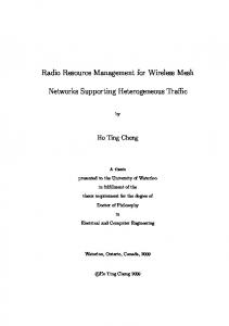
PDES case study WCN simulation case study RRM simulation (MobSim) identification of issues Modeling: - DES/time step - interference radius (case study) FIGURE 1.1.

Synchronization: - mechanism, design, API - state saving - reproducibility

Partitioning: - time - memory

systematic study

Methodology overview.

this reason, we limit ourselves to the constraint of avoiding to introduce additional complexity from what would be typical for sequential simulator development. Modeling complexity has direct bearing on issues dealt with in this study, such as choice of synchronization, design of an Application Programmers Interface for the simulation mechanism, state saving support, and providing determinism in model execution. At this point it would also be fitting with a short discussion regarding research methodology. As has already been stated, the overall framework is that of a case study on simulating RRM in WCNs. Particularly the choice of the RRM problem and the model for this problem is defining for the case study approach. This case is used to identify issues to be dealt with. Nevertheless, once specific issues have been identified these are, in most cases, explored in a systematic fashion rather than only through a case investigation. Figure 1.1 illustrates the concept. In this manner many of the questions and results are generalized beyond the specific WCN model case to a more general PDES setting. Some examples of this include simulation kernel design, state saving, and some aspects of model partitioning and memory usage.

1.4

Thesis Outline

The thesis is organized as follows: The following first four chapters deal mainly with background material. Chapter 2 describes fundamentals of simulation in general, discrete event simulation, and parallel discrete event simulation. Some basic concepts of Wireless Cellular Networks are described in Chapter 3, followed by a discussion of modeling of WCNs in Chapter 4. In Chapter 5 we proceed to discuss related work in the area of parallel simulation of WCNs. This concludes the introductory background part of the thesis. The results part consists of 8 chapters: Chapter 6: We describe the WCN simulation model that we are considering for parallelization in this thesis. This model is also compared with some of the models dis-

5


cussed in the related work chapter, and we show that this model incorporates important features that were not considered in earlier work on parallelization of WCN models. Thus, by investigating this model we enlarge the class of RRM algorithms that could be studied using a parallel model to encompass many new problems of great practical significance. Chapter 7: We describe the MobSim++ experimental platform that is used in experiments in the subsequent chapters. This consists of the PSK synchronization kernel and the MobSim++ simulator running on top of the kernel. Various design and implementation issues are considered, including choice of time advancement mechanism, kernel API, internal design and implementation for transparency and efficiency, and a more detailed look at state saving mechanisms and memory management. While most synchronization kernels are based on either one of shared memory or distributed memory primitives, the PSK can use both to enable the best use of the underlying hardware. It also incorporates the first, as far as we know, published scheme for transparent incremental state saving. At the simulator level, we describe the design and give some examples of use of the Graphical User Interface for visualization of the execution. Chapter 8: One issue concerning the kernel that we encountered relates to determinism and reproducible output in the presence of simultaneous events. This chapter covers this issue in some detail as it turns out to be more complex than it might appear upon first glance. In contrast to other studies on this issue, we relate the problem back to distributed systems theory for a theoretically grounded treatment. Based on this we propose several schemes for slightly different purposes with varying complexity and cost. The cost of one of the simpler schemes is also considered through an empirical study, and as far as we know no other study has presented results on the cost aspect of imposing a scheme for determinism. Chapter 9: This chapter is a prelude to the study of partitioning of the WCN model. Here we consider the influence of the range of interaction between stations imposed by the calculation of interference in the model. The interaction range naturally is an important parameter when considering partitioning later. Experiments are carried out for a case setting to study both simulation fidelity and execution time. The main contribution of this chapter is to take a joint view on model fidelity and execution time and quantify (through experiments) the effects of varying the interference radius parameter in an example model. Chapter 10: One of the crucial problems for parallelization of the WCN model is to find a good partitioning. We study and compare different approaches to partitioning of the WCN model, both through experiments and some limited mathematical analysis. This is the first detailed analysis of the partitioning trade-offs for this type of model. Chapter 11: We investigate the attainable execution time reduction (or speed-up) on a shared memory multiprocessor and consider a number of factors that are known to influence the efficiency of the synchronization protocol. The attainable speed-up is one of the key questions we set out to investigate and we also examine the performance sensitivity to some of the model parameters. A modification to the synchronization mechanism, aimed at exploiting model knowledge for improved performance, is also implemented and evaluated. Chapter 12: The second key question we set out to consider was the issue of memory use for large simulations. We consider the memory use and the possibility of ex6

Introduction

ploiting more available memory on distributed memory machines to scale up the model. As far as we know this issue has not been studied previously for detailed WCN models. We discuss conditions for this model to scale with respect to memory usage in a distributed memory environment, and present some experimental results on distributed memory execution with the aim to exploit more available memory. Chapter 13: This chapter summarizes the results in this thesis, concludes, and indicates possible directions for future work. Also, a list of frequently used abbreviations is given in an Appendix A.

7


8

2 Simulation

Simulation according to Schriber [Schriber, 87] “involves the modeling of a process or system in such a way that the model mimics the response of the actual system to events that take place over time”. Hence, in a simulation study we attempt to estimate the behavior of a physical system by studying a model of the system, i.e. a set of assumptions of how the system works [Law and Kelton, 94]. With the rapid decrease in cost and increase in performance for computers over the latest decades, computer simulation has gained in popularity to become a very important tool for system studies. It carries with it many important advantages compared to other methods but also some drawbacks. When studying a system, be it to gain an understanding of its overall behavior or for performance evaluation of different alternatives, one is faced with a choice of method of study, see Figure 2.1. For an existing system we may choose to study the system directly or to study a model of the system. Experimentation and measurements on the real system offers the best precision and validity of results. However, the costs and risks involved can be prohibitive and in these cases one has to turn to studying an abstraction (model) of the system. For instance, experimenting with the international commercial air traffic system or a nuclear power plant is simply not possible. Furthermore, when evaluating performance while designing or planning a system, i.e. before it physically exists, there is no alternative to modeling. Models can be either physical, e.g. a scale model of an aircraft used in windtunnel experiments, or conceptual/mathematical in nature. Depending on the analysis techniques used, conceptual/mathematical models can be subdivided into analytic models or numerical/simulation models. Analytic models are solved using mathematical symbolic manipulation techniques on the structure of the model and are important in giving

System study

Study on Real System

Physical model FIGURE 2.1.

Study on Model of the System

Analytic model

Numerical / Simulation model

System study method alternatives.

9


Problem Entity Operational Validity

Conceptual Model Analysis Validity and Modeling

Experimentation Data Validity

Computerized Model

Computer Programming and Implementation

Conceptual Model

Computerized Model Verification

FIGURE 2.2.

Simplified version of the modeling process.

a compact high level view of a system. However, if more details need to be added to the model or in cases when certain key assumptions do not hold, it may be difficult to arrive at a tractable model. It is here that numerical or simulation models, solved by a computer, play an important role.

2.1

Simulation Life-Cycle

To understand the pros’ and cons’ of simulation compared to other alternatives it is helpful to consider the simulation life-cycle, as depicted in Figure 2.2 [Sargent, 98]. Building a conceptual model of the system to study, rather than studying the system directly, avoids many problems inherent with direct experimentation and measurements. However, one must now be concerned with the validity of the model, i.e. its correct representation of the system for the intended purpose. Furthermore, when employing computer simulation, the conceptual model must be translated into a representation suitable for a computer, i.e. a program. The correctness of this translation must also be verified. Finally, as in all modeling the output from the model must again be validated against the measured or expected behavior of the system, the so-called operational validity. Adding details, which is usually the motivation for using simulation rather than analytic modeling, not only results in the possibility of higher precision in the results. It also affects all the steps involved in the simulation process. Hence, it may increase the effort needed to validate the model and collect input data, the time taken to implement it on the computer, verify the program against the model, and validate the computer model and input data. And lastly, complex simulation models may require long computer execution times for experimentation. Thus, summing up all these factors there is

10

Simulation

Simulation model

Dynamic (time notion)

Static (no time notion)

Continuous time

Discrete time

time-stepped execution FIGURE 2.3.

event-driven execution (Discrete Event Simulation)

Simulation model taxonomy.

potentially a large increase in the time taken to carry out the study. This must be balanced against the advantage that precision of detailed simulations can typically be improved over analytical modeling. Direct measurement, where it is possible, offers even better precision but is usually even more time consuming [Jain, 91], so simulation represents a middle way alternative. Hence, for an efficient trade-off, it is crucial to balance model detail against the requirements put on the study.

2.2

Simulation Model Taxonomy

Simulation models can be further subdivided based on some key characteristics, as shown in Figure 2.3. Static models represent a view where there is no concept of time. It is either immaterial or the model represents a snapshot view of a time-changing system. For models that include time as a variable one usually differentiate between continuous time models and discrete time models, since these are treated differently. In a continuous time model the system state is defined in all points of time, whereas it is only defined in certain discrete points in a discrete time model. Continuous time models are often described in terms of differential equations, where simulation consists of the numerical solution of these equations. Discrete time simulations are generally executed by having the computer perform discrete time changes to the system model state. If time is advanced in fixed steps of a given size, this is referred to as time-stepped execution. The alternative is to specifically model the occurrence of significant events in the system and advance time with irregular steps between these events. This is referred to as event-driven execution or discrete event simulation. There are also other orthogonal dimensions that can be used to classify models. One is whether or not the model contains randomness. Uncertainty regarding model behavior can be expressed using an element of randomness, in which case we end up with a stochastic model. If there is no stochastic behavior the model is said to be deterministic. To give some examples of this classification: Monte Carlo simulation [Law and Kelton, 94] refers to static stochastic simulation and can be used e.g. to numerically evaluate 11


certain mathematical expressions that are difficult to solve analytically. Discrete time deterministic dynamic models can be used to model e.g. computer hardware systems, and discrete time stochastic dynamic models have many applications including the evaluation of queueing systems that cannot be solved analytically.

2.3

Discrete Event Simulation

In Discrete Event Simulation (DES) [Law and Kelton, 94], the essential features of a physical system are described by a collection of state variables. Changes to the state variables are assumed to occur instantaneously and only at specific discrete points in time. The changes to the system state are specified through the occurrence of an event. For instance, in a queueing system the state could be the number of customers n waiting in a queue and an event E occurring at time t could be the arrival of a new customer, hence increasing n by one. A customer leaving the queue, thereby decreasing n by one, would be the occurrence of another type of event. As mentioned previously, discrete event models can be further classified into deterministic models and stochastic models. For a given set of input parameters the corresponding results for a deterministic model are found by simply executing the model while collecting relevant statistics. In the case of a stochastic model each simulation output represents only one possible outcome of a statistical experiment. Hence, it is necessary to perform a number of replications of each simulation run and use statistical analysis to draw conclusions about the system. The models we will be concerned with in this thesis are all stochastic in nature. Excellent introductions to discrete event simulation and analysis methods for stochastic models are provided in [Law and Kelton, 94] and [Banks and Carson, 84]. When translating the conceptual model into a computer program, the modeler adopts a world view or orientation. The world view may be dictated by the simulation language or package chosen for the implementation or constitutes a design choice when implementing in a general-purpose language. The most common world views for DES are: event-oriented modeling, process-oriented modeling, and activity scanning modeling [Banks and Carson, 84]. The event-oriented and process-oriented world views are the two most frequently used [Wonnacott and Bruce, 96], so we will focus on those here. When adopting an event-oriented view, the modeler codes different event routines to correspond to the different event types occurring in the model. The event routines manipulate the state variables when the event occurs. Events are scheduled to occur sometime in the future either at initiation of the model or by other event routines. The set of future events, the Pending Event Set (PES) or Future Event List (FEL), is maintained by the simulation system so that the next event to occur can be retrieved easily. The execution process mainly consists of extracting the next event, executing it - possibly scheduling new events - and repeating until a stopping condition has been met. Especially for large models the pending event set may become very large, and a well known issue for good execution time performance is to have an efficient implementation of the set [Jain, 91][Rönngren and Ayani, 97].

12

Simulation

A process-oriented model is also based on an underlying event scheduling mechanism but describes the model somewhat differently. A process is associated with each active entity in the model and describes the entity’s actions over time. Thus, the flow of control is interrupted and handed over between the different processes by the simulation system so that all actions by different processes are carried out at the appropriate simulated times. It is often claimed, and stands to reason, that this represents an added level of abstraction over the event-oriented view [Wonnacott and Bruce, 96], thus reducing the model development time. Event-oriented modeling, on the other hand, can be more execution efficient.

2.4

Parallel Discrete Event Simulation

Simulation of complex systems often requires large amounts of resources in terms of CPU time and memory. One possible solution to this problem is to use parallel or distributed simulation techniques. There are two potential benefits from this approach: (i) the execution time of a simulation run could be reduced by execution on a parallel machine, and (ii) more memory could be used by distributing the execution over several nodes or machines. The amount of available memory for large scale simulations is also important from a performance perspective since insufficient primary memory will, in most cases, cause excessive paging and thus dramatically slow down the execution. When contemplating parallel execution to obtain results quicker, there are two possibilities: A straightforward and often efficient way is to run multiple replications simultaneously on separate machines. This is referred to as Parallel Independent Replications (PIRS). The other option is to decompose a single model execution into pieces and have several machines cooperate by executing each piece. This is what we mean by Parallel (and Distributed) Discrete Event Simulation (PDES). For stochastic models that require multiple replications and for different runs to evaluate varying parameter settings, the PIRS approach is oftentimes very useful. Some cautions are in order though [Wong and Hwang, 96]. For instance, if the variance in execution time of a replication is large, depending on the choice of random number seed, it can be difficult to efficiently schedule replications on the available processors. In particular, if n replications are sought one should not continuously start replications on all available processors and collect the n first completed results unless it has been established that the output statistic is not correlated with the execution time. Otherwise, the estimate will be biased as only statistics from the shortest runs have been collected. If different parameter values are investigated the choice of parameter settings is sometimes best made based on results from previous runs, thus imposing some sequencing dependence between runs. Without access to these results some of the scheduled runs using PIRS may be wasted. Furthermore, n parallel replications require n times the memory of a single replication. So, if there is not sufficient physical memory for a single replication on a single node, the PIRS approach is of limited use. PDES has the potential of facilitating the execution of larger models, making use of the memory of several machines for a single run. It could also help in cases with sequencing dependencies between runs. Moreover, the issues encountered in PDES research are valid for, and can be applied to, other areas within computer science, 13


Time State-variables over simulated time

t6 t5 t4 t3 t2 t1 0 S1

S2

S3

S4

State - Subsystems FIGURE 2.4.

Execution of a simulation viewed over the space-time plane.

especially in the realms of parallel and distributed systems technology. The often highly dynamic behavior of the simulation applications pose some of the most challenging issues for parallel computation research, so there is a motivation for PDES research from a broader theoretical perspective. For instance, issues regarding synchronization, partitioning, and load balancing are highly complex in the PDES setting. In this section we will focus on the synchronization problem which is something of a root problem, from which the field has sprung. Partitioning will be discussed more in Chapter 10 and Chapter 12. The synchronization problem has also been encountered from a somewhat different starting point. With the development of interactive simulations for training, mainly in the military arena, the desire to connect several simulators into larger distributed training exercises emerged. This led to the development of distributed interactive simulation (DIS) protocols. Having the starting point from interactive simulations with real-time demands, these protocols focused on the exchange of data between simulations without regarding guarantees of causal correctness. These efforts later resulted in development of the High Level Architecture (HLA) which is meant to enable interoperation and distributed execution of simulation models. Within HLA, the Time Management Services of the Run-Time Infrastructure support synchronization of simulation data exchanges [Dahmann et al., 98]. HLA specifications provide different options for time management, ranging from no causality-guarantees to guaranteed causal correctness for data delivery. These developments have led to the incorporation of ideas from the PDES field. In Parallel Discrete Event Simulation (PDES), a DES model is partitioned to run on several processors of a parallel machine or distributed over a network. Figure 2.4 shows execution of a simulation over space-time, where the general simulation problem amounts to filling in the simulation state over time [Fujimoto, 90b]. In this diagram it is assumed, which is often the case, that the physical system can be viewed as a set of disjoint subsystems each with a disjoint set of state variables. As can be seen in the diagram there are, in principle, two ways to partition a simulation execution: along the time axis or along the state-space axis. In practice usually only the initial conditions, 14

Simulation

Message with lowest time-stamp Select for processing! 1.2

7.3

Logical Process

5.6 FIGURE 2.5.

The causality principle can be upheld in a conservative synchronization scheme by always selecting the message with the lowest time-stamp for processing, provided that there is at least one message in each input channel.

i.e. state at time t=0, are known making a time partitioning impossible. Although, in some cases, by exploiting the special properties of some systems, it has been possible to accomplish a time partitioning (some examples are listed in [Fujimoto and Nicol, 92]). By far the most widely used approach is to partition the simulation along the statespace axis and model each subsystem by a logical process (LP), such that LPi corresponds to Si. Hence, the simulation model will be composed of N (N>1) communicating LPs with disjoint states. In DES all events have an associated time-stamp indicating at what simulated time the event should occur. In a sequential simulation the events are processed in time stamp order to ensure that an event cannot affect its past history (if this should occur it is known as a causality error). In PDES, each LP asynchronously processes events in parallel with the other LPs. Thus, instead of a centralized clock, the LP has its own logical clock, the Local Virtual Time (LVT), that runs independently of the other LPs. For this reason, the LPs have to be synchronized to avoid causality errors. Mechanisms proposed to handle this problem fall roughly into two categories: conservative and optimistic synchronization schemes [Fujimoto, 90b].

2.4.1 Conservative Synchronization Conservative schemes ensure that only safe events are processed so that causality errors never occur, while optimistic schemes use a detect and recovery mechanism in the case of a causality error occurring. An event is safe to process if it can be guaranteed that no message (i.e. event) with a lower time stamp will arrive at the LP at a later time. This can be accomplished e.g. by using static communication paths between the LPs with order preserving communication channels. Given this and a queued message on each of the incoming channels to an LP, as shown in Figure 2.5, it is sufficient to pick the message with the smallest time stamp to guarantee causal correctness. This is the essence of the Chandy-Misra algo15


rithm [Misra, 86] which was one of the first algorithms proposed for synchronization of parallel discrete event simulation models. Since it is required that at least one message exists on each channel there is a potential deadlock problem. Consider the case of a circular connection where each LP will wait indefinitely for its predecessor. Different schemes have been proposed to deal with the deadlock problem. One frequently used scheme is to send null-messages that serve only as a lower bound on the earliest arrival time of a future message on the channel. Thus, the reception of a null-message can help the synchronization mechanism to detect that some of the other messages are, in fact, safe. However, depending on the model characteristics, the proportion of null-messages to “real” event messages may be large, resulting in large overheads. Other proposals avoid the deadlock problem by proposing a different approach for conservative synchronization. Window based protocols compute safe time windows. The events within a window can be processed safely in one phase after which processing is stopped and a new time window is computed in the next phase. Both null-message sending and computation of safe time windows require some knowledge about the future event-scheduling behavior of the model, i.e. some knowledge of the future in the model. This information is referred to as look-ahead information. The amount of look-ahead information available is highly model dependent and the system usually has to rely on the modeler to supply this information. However, in certain cases it has been demonstrated that look-ahead information could be extracted automatically by the simulation system, see e.g. [Nicol, 88]. The reader is referred to [Fujimoto, 90b] for a more in depth discussion of conservative synchronization schemes including window based protocols.

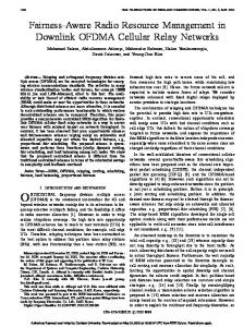
2.4.2 Optimistic Synchronization A criticism that has been raised against conservative synchronization is that there could be many cases where events might be correctly processed but a conservative protocol blocks unnecessarily because it is not able to guarantee correctness. Thus, it might not fully exploit the available parallelism in the model. Another approach, targeting this issue, is represented by optimistic synchronization mechanisms. Here one optimistically assumes that the incoming messages can be sorted into an in-queue and thereafter processed immediately, as it is expected that they will arrive approximately in time order. However, this requires a mechanism to detect and correct for situations when this assumption fails. Figure 2.6 illustrates the workings of this mechanism. A causality error is caused by a message arriving at an LP with a receive time-stamp that is smaller than the current LVT of the LP. In optimistic schemes, where this may occur, such a message is called a straggler message. To be able to recover from a causality error in optimistic methods, i.e. perform a rollback, it is necessary to do two things: (i) the LP must restore its state to a point preceding the receive time of the straggler message to undo erroneous computation, (ii) the effects of all messages erroneously sent since the receive time of the straggler message must be undone. Restoring an earlier state of the simulation can be accomplished if the state of the simulation is saved periodically during forward execution. This leaves us the problem of messages erroneously sent out. In the Time Warp mechanism [Jefferson, 85], which is the most well known optimistic method, erroneously sent messages are neutralized by the sending of a matching anti-message. The ar16

Simulation

1. straggler message Logical Process A

5.4

input queue

output queue 3. antimessage sent based on message in output queue, an anti-message is sent to cancel it

5.5 6.1

5.9

event set LVT: 5.6

5.3 5.6

-6.1

state set

Logical Process B

5.3 5.6

input queue 2. rollback: - set LVT back to 5.4 and restore state at 5.3 - insert straggler event - cancel messages sent by event at 5.6

output queue

6.1

event set

state set

4. cancellation the antimessage eliminates the positive message in the input queue or triggers a new rollback if the message has already been processed FIGURE 2.6.

Example of rollback in optimistic synchronization.

rival of an anti-message to an LP annihilates the corresponding positive message and will, if the message has been processed, consequently trigger another rollback and give rise to more anti-messages being sent out. Since the mechanism requires the saving of data in case of future rollbacks: state history, processed events and sent messages, an important consideration is how and when to reclaim this memory. Consider one specific datum, be it state, event, or message. It is clear that once the simulation (in all LPs) have progressed to a point such that no rollbacks could occur back to the time associated with the datum, then it could be reclaimed. To determine this condition we need to compute the lower bound on all LVTs in the different processes and the send times of all messages in transit, the global virtual time (GVT). The system can periodically compute GVT and then fossil collect memory up to the GVT. Although, in practice one often has to settle for an estimate ˆ of the GVT, such that GVT ˆ ≤ GVT . GVT Many algorithms have been proposed for estimating GVT with a tight bound and at low cost. The problem can be reduced to the general problem of finding a snapshot of the distributed computation, i.e. a global state consisting of process states and communication channel states such that they could have been recorded simultaneously. The GVT can then be estimated for the snapshot instance. General GVT algorithms, based 17


on the notion of consistent cuts, are given in [Mattern, 93]. For FIFO communication channels, a simplified algorithm is proposed in [Lin, 94]. On a shared memory machine, a consistent cut (and hence a snapshot) can be obtained in a straightforward fashion and at low cost through a barrier synchronization. This greatly simplifies the problem but has the drawback that it is inhibitory, i.e. it stops the computation. Asynchronous (non-inhibitory) algorithms have also been developed that are optimized for shared memory, e.g. [Xiao et al., 95].

2.4.3 Issues and Optimizations There are a number of obvious overheads and performance liabilities associated with optimistic synchronization, both in terms of time and space. Many techniques have been proposed to optimize various aspects of the optimistic mechanism. Here, we will only mention a few of the more central ones. Known issues for good performance include: • state saving • antimessages - cancellation policy and implementation Also, the issue of memory consumption goes beyond only achieving good performance. It is known that unconstrained optimistic execution can consume memory to the point of memory exhaustion preventing further progress. So, in order to ensure that the simulation can run to completion special protocols are required to manage memory usage. In the rest of this section we will discuss each of these issues. Efficient state saving is known to be an important issue for good performance [Fujimoto, 90b] and several techniques have been proposed to deal with this problem. In fact state saving is perhaps something of a misnomer since the proposed techniques utilize either state saving, state reconstruction, or a combination of the two to achieve good efficiency. Figure 2.7 illustrates the principal methods to save and restore state information. The most straightforward method is to copy the entire state of the LP after each event execution, i.e. copy state saving (CSS). State can be restored for any previous time by copying back the saved state. Obviously, this will be costly for large state sizes. One way of reducing the cost is to only save state periodically, through so called sparse state saving (SSS) or infrequent state saving. In case the desired state has not been saved, a prior state is restored and forward coasting, i.e. reexecution without message sending, is used to reconstruct the desired state. The challenge here is to find the optimum state saving interval to balance state saving and restoration costs. Several schemes have been proposed and we discuss this in some more detail when discussing state saving implementation in the experimental platform in Chapter 7. If the state is large it is frequently only a small portion of the state that is modified in each event. A more efficient alternative is then to only save the portion of the state that was actually modified. In incremental state saving (ISS) a chain of state modifications, backwards chained, is built so that state can be restored by traversing this chain in reverse order [Cleary et al., 94]. A hybrid approach using sparse state saving and backward chaining increments has also been proposed for situations when it is desirable to bound the state restoration cost [Gomes et al., 97]. Finally, it has recently been proposed [Carothers et al., 99] that for operations that are constructive, i.e. that can be reversed, and in cases 18

Simulation

- executed event

- state

- unexecuted event 2. state reconstruction time

time

state restore

1. state restore

Sparse State Saving

Copy State Saving

time

time

state reconstruction state restore Incremental State Saving

FIGURE 2.7.

Reverse Execution

State saving methods.

where the computation cost is small (compared to state saving) it could be efficient to perform reverse execution to reconstruct the state. However, since many operations are irreversible, this must be supplemented with incremental state saving to fill in the gaps. Regarding antimessages, there is a design-choice of whether to let rollbacks propagate aggressively or lazily. When using aggressive cancellation, antimessages are immediately emitted when performing the rollback in order to stop erroneous computations in other LPs as quickly as possible. The other alternative is to delay the sending of antimessages until it can be determined whether the rollback actually results in different messages being sent out. It is conceivable, after all, that some or all of the generated messages remain identical even after processing the straggler depending on how it affected the state. Thus, in lazy cancellation [Gafni, 88] we instead decide during forward reexecution if some, or all, of the messages generated by reexecution are identical with the previously sent messages. If so, there is no need to cancel the previously sent message, thus saving antimessages and possibly rollbacks. If this speculative strategy is successful it could, in the most favorable circumstances, even lead to supercritical speed-up, i.e. execution faster than the critical path [Jefferson and Reiher, 91]. However, the downside is that erroneous computations may propagate further since cancellations will be delayed. Rapid halting of erroneous computation paths is important for efficiency and in certain cases even for progress of the execution. It has been

19


pointed out that in certain cases of cyclic LP dependencies, if cancellation and rollback are not faster than forward progress, the execution could live-lock. The implementation of antimessages can also be optimized in the case of execution on a shared memory machine. On distributed memory, an antimessage that is sent must be matched up with the positive message by the receiver. Thus, the receiver must search the positive messages in order to be able to annihilate the correct one. On shared memory, the antimessage can simply consist of a pointer to the positive message, retained by the sender. Locating the positive message for cancellation is then trivial, reducing the cost. This optimization is referred to as direct cancellation [Fujimoto, 89b]. Finally, we consider the problem of memory stalls. Several different methods have been proposed for dealing with the problem of memory stalls in parallel simulations, i.e. a situation where memory is exhausted thereby preventing further progress. This is an important problem since, if no special actions are taken, a memory stall will lead to premature termination of the execution. Protocols proposed to handle memory management in Time Warp include Gafni’s protocol [Gafni, 88], cancelback [Jefferson, 90], and artificial rollback [Lin and Preiss, 91]. These protocols all recover from memory stalls by rolling back some possibly correct computations to free up memory to enable forward progress. A memory management protocol is said to be optimal if it can guarantee that the simulation can be completed in constant bounded memory, i.e. within a constant factor of the memory required for sequential execution. Cancelback and artificial rollback have been shown to be optimal in this sense. In order to ensure optimality they both assume execution on a shared memory system and maintain a global view of the machine. In cancelback, the basic idea is to define appropriate actions to allow removal of an item from memory: a message in an output queue, a message in input queue, or an LP state. A message in an output queue can be removed provided that the corresponding message in the input queue of the receiver is canceled. As usual this may involve rolling back the receiver. A message in an input queue can be removed by sending it back to its originator to cancel out the corresponding antimessage stored in the output queue. The sending event needs to be rolled back in this case. Finally, a saved state can be removed by rolling back the computation of the corresponding LP. Only items with sendtimes greater than GVT can be removed. Before GVT there is no information stored to support rollback, and removing items exactly at GVT could induce a livelock situation [Lin and Preiss, 91]. It should also be noted that the “sending back” of messages in the input queue to the sender acts as a form of flow control between LPs, thereby stopping other processes from progressing too far and exhausting the memory. One potential problem regarding this protocol is also noted though. It is possible that a reverse message causes the sender to rollback, re-execute, and then resend, only to find that there is still not enough memory available to receive the message. This could lead to another reverse message, re-execution, resend, and so on. This could be repeated any finite number of steps and is referred to as “busy cancelback”. The artificial rollback protocol is designed to be easier to implement than the cancelback protocol and more efficient in some respects. In each step taken to release memory, a set of victim LPs is selected (globally), and artificially induced to roll back. The victims are selected to be the processes with the largest LVTs. If the released memory is not sufficient, each successive step will proceed backwards to select victims with 20

Simulation

lower virtual time. The artificial rollback mechanism is considered to be easier to implement and more efficient since the proposed coordinating mechanism is less intrusive on the processes than cancelback, and the concept of an artificially induced rollback does not require implementation of new cases to deal with reverse sending of messages. Furthermore, the protocol also specifies a scheduling policy to deal with the problem of busy cancelbacks.

2.4.4 Extensions and Hybrids Conservative synchronization and optimistic synchronization, as in the Time Warp scheme, represent two fundamental approaches. But these are, by no means, the only options. In [Reynolds, 88], Reynolds defines eight design variables that can be used to characterize PDES synchronization protocols: Partitioning (referring to heterogeneous synchronization within a model, not model decomposition), Adaptability, Aggressiveness, Accuracy, Risk, Knowledge embedding, Knowledge dissemination, Knowledge acquisition, and Synchrony. Particularly the notions of aggressiveness and risk can be helpful when thinking about extensions and hybrid protocols. Aggressiveness refers to speculative processing of messages in a process. Risk, on the other hand, refers to the sending of messages based on speculative processing, i.e. messages that may have to be cancelled. Thus, e.g. the Chandy-Misra scheme is non-aggressive and risk-free, whereas Time Warp is both aggressive and risky. Other protocols have been proposed that limit the amount of risk, or risk and aggressiveness, either adaptively or non-adaptively. For instance, the SPEEDES system [Steinman, 92][Wieland et al., 95] lets the user specify, through parameters, the maximum number of events to process speculatively and messages to send risky. Several mechanisms have also been proposed to adaptively bound the aggressiveness of Time Warp, based on LVT [Ferscha, 95], event counts [Panesar and Fujimoto, 97], or memory usage [Das and Fujimoto, 94]. Starting from the other direction, elements of aggressiveness may be added to a conservative protocol, as in [Dickens and Reynolds, 90]. Lastly, schemes using different synchronization strategies for different parts of the simulation (partitioning in Reynolds’ terminology) have also been proposed, e.g. in [Rajaei et al., 93]. Knowledge dissemination and acquisition refer to “push” and “pull” diffusion of knowledge that let LPs progress. Hence, e.g. null-messages in the Chandy-Misra scheme constitute an instance of knowledge dissemination. Synchrony denotes whether processes progress completely asynchronously, synchronize globally from time to time (loosely synchronous), or completely synchronously (e.g. time-stepped).

21


2.5 Concluding Remarks The choice of synchronization mechanism is not obvious, and usually has to be made on a per application basis. Where conservative schemes may err on the side of caution, leading to excessive blocking, optimistic schemes may suffer from excessive rollback overheads. Furthermore, optimistic schemes have known issues such as the need for efficient state saving methods that are often crucial for good performance. Conservative schemes, on the other hand, must detect safe events and rely heavily upon look-ahead, the ability to foresee the future in a simulation, to obtain good performance. The availability of look-ahead information is highly application dependent and by placing the responsibility of supplying this information mainly on the modeler, it may complicate model development. No single approach to synchronization has yet been shown to provide good performance for all applications, and it is unlikely that this will ever happen. Instead, in [Lin, 93], Lin advocates the development of tunable simulation environments that should be easy to use for naive users, but possible to modify for the advanced user to obtain optimum performance.

22

3 Wireless Cellular Networks

The overall goal for emerging mobile and personal communication services is to enable communication with a person, at any time, at any place, and in any form [Pandya, 97]. Different initiatives such as the U.S. Personal Communication Systems (PCS) standard, the European GSM standard, and the Japanese PDC system, have been deployed in large scale and form the second generation of systems designed towards meeting these goals. Future generations of systems are already in the pipeline to meet demands for other forms of communication than speech traffic. Different techniques are employed in different systems to achieve these goals but one that is central, and thus of great practical importance, in providing mobile user access to fixed communication networks is based on wireless cellular networks. Cellular networks are used in all of the above mentioned systems for a combination of good coverage and high capacity. In the continuing discussion, we further restrict ourselves to dealing only with radio based systems, i.e. cellular radio networks, as it is the predominant technology.

3.1

Cellular Radio Networks

A cellular radio network provides access for users within a specific service area, and this region is populated by a number of base stations (BSs), see Figure 3.1. The radio coverage of a BS is called a cell. Due to obstacles in terrain etc. cells are irregularly shaped and generally overlapping, but occasionally with spots lacking coverage altogether [Ahlin and Zander, 98]. Users carrying a mobile terminal (MT) can communicate with other parts of the system by transceiving with the BS covering the cell they are located in at that specific time. For duplex communication we also require separate communication channels for uplink (MT to BS) and downlink (BS to MT). The terms mobile terminal (MT) and mobile station (MS) will be used interchangeably throughout this thesis. Cellular radio networks are complex systems and many issues must be addressed in their design, both regarding the air interface and the fixed network part connecting it to a wired backbone network. The radio medium imposes many problems at different levels due to propagation path loss and interference. Link level considerations include e.g. signal modulation and coding for efficiency and error resistance. On a network level we must also consider multiple access techniques and radio resource management. Relating to both radio and fixed network parts are issues such as call control and mobility management. Jabbari, in [Jabbari et al., 95], names issues related to radio resource assignment, mobility management, and call control, as having significant impact on network performance. In this study we focus on radio issues on a network level and this 23


BS

network service area FIGURE 3.1.

fixed network part

Cellular Radio Network.

section will just briefly give some background on some of the issues present. The discussion of radio resource management is based largely on [Zander, 96] and [Ahlin and Zander, 98].

3.2

Multi-User Communications

The spectrum band available to the system, as allocated through national agencies, must support multiple concurrent users. Multiple access schemes provide a means of separating the signals from different users for the receiver. The majority of currently deployed systems are based on Frequency Division Multiple Access (FDMA), Time Division Multiple Access (TDMA), or a combination of the two. Here, orthogonal communication channels are defined for different users and for uplink (mobile-to-BS) and downlink (BS-to-mobile). In FDMA, a (narrow) frequency band is allocated to each channel and the receiver tunes in to this frequency band, filtering out other signals. In TDMA, channels are defined through time slots on the signal. Combinations (F/TDMA) consisting of time slots on different frequency bands are used e.g. in the GSM system. An alternative is to use spread spectrum, or Code Division Multiple Access (CDMA), techniques where the transmission is spread out over the available spectrum to improve resilience to frequency selective fading and interference. This advantage, known as a form of diversity gain, comes at the price of more complex implementation. Frequency Hopping (FH) resembles F/TDMA in the division of time and spectrum, but here the transmitter (and receiver) hops between the different frequencies in each time slot in a predefined sequence. In Direct Sequence-CDMA (DS-CDMA) the signals of different users are coded so that the receiver can isolate the desired signal through a decoding step.

24


3.3

Radio Resource Management

Since available radio frequency spectrum is limited, it is important to utilize it efficiently. For this reason, radio waveforms are reused in different cells in the system. This can be done as long as different users are sufficiently spaced apart, to ensure that interference caused by transmission by other users (elsewhere) will be negligible. Thus, we require some form of channel assignment strategy for the system to ensure a sufficient reuse distance and low interference. As MTs move around it may become necessary to switch an ongoing call over to another BS or to use another channel on the same BS, this is referred to as a handover (HO). When moving closer to the BS, the same received signal strength can be upheld for a lower transmitted power. Thus, the transmission power can be reduced, so called power control. Apart from extending battery lifetime in the terminal, this has the added and possibly more important benefit of decreasing the amount of interference caused to other users in the system. The problem of Radio Resource Management (RRM) [Zander, 96], which is targeted in this study, is that of selecting for each ongoing call: • base station • radio waveform • transmission power so as to maximize the carried traffic while maintaining the Quality-of-Service constraints. The maximum carried traffic is a measure of system capacity. So what are the Quality-of-Service constraints? For call traffic our concerns are to be able to initiate a new call, and to maintain it with acceptable speech quality. The first issue we consider is coverage. The outage probability is a measure of the fraction of time a signal is below the required threshold for communication due to adverse propagation conditions. The second issue is assignment failure, i.e. we are not able to assign radio resources to provide a usable communication link. Let us assume, for simplicity, that the transmission quality (e.g. bit error rate) is only dependent on the (local average) Signal-to-Interference Ratio (SIR). Thus, we assume that communication can be upheld as long as the SIR Γ i (or actually signal-to-interference-and-noise ratio) is above some minimum threshold γ o for both uplink and downlink. Consider the uplink from MTj to BSi, then this constraint is written as: P j ⋅ G ij Γ i = -------------------------------------------- ≥ γ o P m G im θ jm + N

∑ m

where P j is the transmitted power, G ij is the link gain, and N is the received thermal noise power. The sum in the denominator is the total received interference from other transmitters (MTs) in the system, where θ jm is the normalized crosscorrelation between signals from MTs j and m. The radio waveform for the signal, mentioned in

25


the problem definition, is the channel in the case of F/TDMA. For orthogonal channels (e.g. orthogonal F/TDMA) there is no crosscorrelation between channels, thus:  1 if j and m are using the same channel θ jm =  otherwise 0 In this study we will focus on systems that are interference- rather than range-limited, i.e. where interference from other users is the main limiting factor rather than system coverage. Hence, our main focus is assignment failures, and these could occur when initiating a new call or during the course of a call. An attempt to initiate a call may fail because there are no available channels in the cell. This is referred to as a blocked call. Similarly a HO may fail, due to unavailability of channels, which may result in poor reception for the MT for a prolonged time and eventually causing the call to be terminated. Such a forced termination is termed a dropped call. The probabilities of blocked and dropped calls at a specific system load are used as Quality-of-Service measures for the network. The blocking and dropping probabilities should typically be kept below 12%. Performing RRM is the task of the Resource Allocation Algorithm (RAA), and we want to design a simulation model that can be used to evaluate and compare RAAs. Consequently, this includes algorithms for channel assignment and power control in the system, but also call admission control and handover strategies. Different schemes exist to assign channels to cells to ensure sufficient SIR. In Fixed Channel Assignment (FCA), the assignment is performed statically at system design time. In principle we wish to obtain a sufficient channel reuse distance to cater for the “worst case interference”. The available radio channels are divided into K disjoint subsets, channel groups. Correspondingly, K neighboring cells are grouped into a cluster and a channel group is assigned to each cell in the cluster. By adjusting the size of the cluster, the required reuse distance can be obtained. It is obvious that if there are fluctuations in the traffic in the system over time, FCA may not provide an optimum allocation of resources. Dynamic Resource Allocation algorithms strive to improve resource utilization compared to static assignment by dynamically reassigning resources based on real-time measurements of the status of the system. Dynamic Channel Assignment (DCA) schemes have been shown to be able to improve channel utilization compared to FCA by exploiting different types of knowledge to dynamically reassigning channels among cells. Algorithms may try to adapt to the instantaneous traffic distribution (number of MTs) in the system, or to the received power level, or to the measured interference and noise level. A Traffic-Adaptive Channel Allocation scheme performs DCA based on measurements of the number of active MTs in different cells and conservative estimates (similar to FCA) on required mutually exclusive use of channels between cells. That is, the channel usage constraints take the form “if a channel is used in cell a it cannot be used in cell b, and vice versa”. Channel Borrowing schemes are hybrids between full trafficadaptive DCA and FCA, where some of the channels are statically assigned and a pool of channels can be reassigned. Reuse Partitioning schemes use multiple overlaid cell plans to exploit the fact that MTs close to the BS generally have higher average SIR than MTs close to the cell border. Thus, they are essentially a refinement on FCA and 26


can also be combined with traffic-adaptive DCA. Hence, in this case they constitute DCA schemes that also exploit differences in received interference, but they are essentially based on conservative predictions in a similar manner to static cell plans. Finally, Interference-Adaptive Channel Allocation schemes avoid using conservative estimates by measuring, in real-time, the received interference (and noise) to select the most favorable channel. In addition to channel assignment we also need to select an appropriate transmitter power. We have already noted that by reducing the transmitted power in favorable conditions, the interference caused to other users can be reduced. Thus, by performing Power Control individually per link it is possible to increase system capacity. Algorithms have been proposed aiming to either maintain a constant received power level or to balance the SIR in the system. The idea behind SIR balancing power control is to adjust power to provide a usable communication link, i.e. a sufficient SIR, to as many (simultaneous) users as possible in the system. Finally, HO mechanisms to select and switch between BSs to communicate through will have an impact on the resource utilization in the system, and different mechanisms have been proposed and investigated. It has also been noted that signaling due to mobility management, for instance, (i.e. keeping track of where MTs are) can have an impact on the RRM. That is, more frequent HOs to efficiently use BSs will cause more signaling for mobility management, leading to a possible trade-off.

3.4

Discussion

The RRM problem is our main focus in this study, but when contemplating the simulation model later, a desirable property was also to be able to include some elements of signaling in the model to evaluate trade-offs, such as those resulting from mobility management. In fact the MONSTER model, discussed later, which was one of the main influences at the outset included some levels of signaling related to resource management and call control. Call control signaling meaning e.g. signaling for intercell HOs (between cells) and intracell HOs (to another channel on the same cell). It is also important to note one additional aspect of RAAs in relation to this study: Algorithms differ not only in the type of information that is exploited, but also in how much information is used to make a decision. Centralized algorithms are based on the assumption that the cost of sharing information in the system is low or negligible, so system wide knowledge can be used by a centralized entity to make RRM decisions. However, in practice there is a cost associated with disseminating information, and consequently distributed algorithms (that use only local information) are generally sought for real implementations. When considering parallelization of a simulation model of the system there is a similar cost associated with collecting global information in the system. Thus, intuitively one would expect that simulations of distributed RRAs should be easier to parallelize than centralized algorithms. Since the information is used only locally in distributed algorithms, more independent actions are performed in different parts of the system and consequently there should be more available parallelism in the model.

27


28

4 WCN Models

With all the different issues of the previous chapter in mind, it is clear that a WCN may be modeled at many different abstraction levels and using various techniques to target the specific questions. In this chapter we start by discussing modeling of WCNs at some different levels of abstraction, regardless of analysis method. This is not meant to be a comprehensive enumeration, but serves as a frame of reference for a discussion on simulation models and tools. Focusing then on simulation, we proceed to discuss both general purpose and more application specific simulation tools and models. This concerns the tradeoffs made when selecting a tool and the typical modeling concepts used in the area of communication networks. Thus, this chapter provides the necessary background information to relate efforts in parallelization of WCN models (described in the next chapter) with some existing sequential simulators. Specifically, it provides the background for discussions on the applicability of different parallel simulation approaches to different types of models.

4.1

Abstraction Levels

When discussing descriptions of communication systems at different levels of abstraction, a possible starting point could be given through the protocol architecture. The open systems interconnect (OSI) model was developed as an international standard model for a computer communications architecture [Stallings, 97]. The model consists of seven layers, depicted in Figure 4.1. Especially the three lower levels can provide a frame of reference when discussing modeling of the system. Application Presentation Session Transport Network Data Link Physical FIGURE 4.1. OSI model protocol architecture. 29


Models of the Physical and Data Link layers are typically used to study e.g. modulation and error correction coding performance over a single communication link. Moving upwards to the Network layer, we may design models to study e.g. resource allocation in the network while abstracting away most of the details of the lower layers. Models of higher layers are frequently used to study functionality or performance of the corresponding protocols, but may abstract away characteristics of the physical network such as topology. In this thesis we focus on network level issues, as opposed to single link models, possibly with the addition of higher level protocols. Also when confining ourselves to network level issues and descriptions, the system may be studied at different levels of abstraction. Furthermore, different approaches can be preferable depending on whether we are focusing on the air interface or the fixed network part of the system. Let us proceed by considering modeling of the air interface.

4.1.1 Cell-Level Modeling A high-level description of radio resource management in the system can be obtained by assuming that all cells in the system have a regular, homogeneous, shape and the service area is covered through a tessellation of such cells [Ahlin and Zander, 98]. Common assumptions are hexagonal cell or quadratic cell meshes as shown in Figure 4.2. Especially the hexagonal mesh is popular since the shape of a cell most closely approximates a circle, thus resembling free-space propagation. In this thesis we call models using this assumption “cell-level” models since system topology is described only down to the level of cells. By modeling the arrival and departure processes of calls to the system, spread over the service area, and the user movements between cells (HOs), we can study methods for allocation of radio channels at a high level of abstraction. FCA schemes can be compared e.g. with DCA schemes based on “channel-borrowing” between cells.

FIGURE 4.2. 30

Examples of hexagonal mesh and quadratic mesh cell layouts.

WCN Models

1

3

FIGURE 4.3.

1

2

4

Cell coverage is irregular due to obstacles in the terrain, resulting in partially overlapping cells and possibly uncovered areas.

Cell-level type models have been used in a number of studies to evaluate these aspects of proposed radio resource management strategies. Some examples are [Kuek and Wong, 92] that use a one-dimensional model and [Zhang and Yum, 89] that use a twodimensional model. At this level the model resembles a connected queueing network where each cell is a queueing system and the number of servers is equal to the number of radio channels available in the cell. While an FCA system might thus lend itself to analytic solutions in this manner, it can be harder to capture dynamic reallocation of channels. This type of assumption represents a great simplification of the real systems since signal propagation effects of the terrain will cause cell shapes to be irregular, mostly overlapping, and sometimes discontiguous, as shown in Figure 4.3. Consequently, more detailed models are typically required for network planning. Moreover, several aspects of RRM cannot be studied at this level of abstraction. Since there is no concept of signal strength, either for the desired signal or interference, power control algorithms or measurement based channel assignment cannot be studied.

4.1.2 Propagation Modeling Static models (see Section 2.2) of radio propagation, i.e. focusing on the physical level of radio propagation, provide a more detailed view and can be used e.g. for network planning purposes. The objective in this case is to predict the signal path loss at different points in the service area to determine the coverage of a given system configuration. Engineers designing and installing systems need effective tools to help them determine appropriate locations for base stations to provide good and efficient coverage of the service area. Computerized propagation prediction tools, based on this type of static models, are commercially available to provide this support. An example of a propagation prediction tool is described in [Wagen and Rizk, 93] that takes reflection and diffraction phenomena into account to predict propagation in urban environments. Another tool focused on indoor systems, that also includes optimization tools to help in placement of base stations, is described in [Fortune et al., 95]. A different example of usage is given in [Phongphanphanee et al., 99], where this type of model is one component in a study exploring the possibility of utilizing existing indoor systems to also provide outdoor coverage in an urban environment.

31


4.1.3 Channel-Level Modeling Let us turn back to consider RRM issues again. Propagation models deal with the physical layer of the radio channel. RRM studies, on the other hand, deal with the allocation of resources to traffic in the network, i.e. at the network layer. By combining dynamic aspects i.e. teletraffic and user mobility elements, as in the cell-level models, with models of radio channels, cf. the static propagation models, one can arrive at a highly detailed model that can be used to study e.g. power control and perceived interference for RRM schemes. In fact, the [Phongphanphanee et al., 99] study mentioned previously also incorporates teletraffic and mobility models to evaluate the quality of service provided by the system. However, many different approaches can be used for channel modeling and they do not necessarily employ the same techniques or the same level of detail as the models used for propagation prediction. It can be useful to make a distinction between verification models and design models at this point [Ahlin and Zander, 98]. While a very detailed radio channel model for a specific situation is useful for verifying system performance in that situation, a more abstract and general model can be more useful for system design. Consider a radio communication channel for mobile communication. Due to user mobility, the properties of the channel, as perceived by the receiver, will vary over time. The channel is said to be time-variant. A reasonable alternative to that of using a static model for a specific physical setting is to characterize the dynamically changing channel statistically. Thus, the general characteristics of certain phenomena can be abstracted, generalizing it from a specific situation. The statistical properties of effects such as shadow fading, due to obstacles, or multi-path fading, due to interference from multiple reflected signals, are typically described in such a model. But exactly what is included in the model naturally depends on its purpose and the characteristics of the system. Depending on timing characteristics, for instance, it might be important to also capture signal delay spread information to include inter-symbol interference. By including certain elements of the physical channels into the network model in this manner, one can go beyond the issues covered through cell-level models. Nevertheless, as some examples will illustrate the level of detail included in the model may vary, as may the treatment of time. Static models (Monte Carlo) may be used to study power control or channel assignment in a system snapshot situation, as in [Grandhi et al., 94]. In this study the channel model considered only the distance dependent fading through an exponential power decay law. A distributed power control scheme was proposed and its performance was examined through the snapshot model. Dynamic simulations are performed e.g. in [Cheng and Chuang, 96] to study power control and measurement based DCA. In their model they also include a statistical model of (long-scale) shadow fading on the radio channel. This is modeled by superimposing a log-normally distributed stochastic fading on the distance dependent fading. A dynamic teletraffic simulation including this channel model is used to evaluate two different measurement based algorithms for DCA. For dynamic models, some time advancement mechanism is needed and models at this level might be efficiently simulated using either time-stepping or event-driven execution. We will return to this in later chapters.

32

WCN Models

4.1.4 Protocol-Level Modeling Proceeding upwards through the protocol stack, we can add protocol levels or shift focus towards higher level protocols to study their functionality or performance. For instance the protocols governing resource management and call control might be interesting to include in a resource allocation study. Protocols at a higher level, e.g. for user authentication, probably do not require as much information about the network, so for instance topology might be abstracted away. One such example is [Kesdogan and Fouletier, 95] where protocols for secure location management are studied. An important point to be noted here is that protocols of this type are generally asynchronous in nature, and therefore usually more efficiently simulated using event-driven rather than time-stepped execution.

4.2

Simulation Tools and Models

The selection of a proper tool or language is probably the most important step in the process of developing a simulation model [Jain, 91]. We have already touched upon some of the software tools that have been proposed or are available to study the different types of models considered. Let us look at this in some more detail, but now focusing on dynamic models. We start from the lower layers as before, by briefly mentioning some of the tools available for link-level simulation. A more extensive discussion then follows on network simulation. Here we consider general tools for discrete time simulation, specifically DES, of communication networks and then proceed through more and more specialized tools and models for radio networks and RRM.

4.2.1 Link-Level Simulation Commercial simulation tools such as COSSAP (Communication Systems Simulation and Analysis Package) from Synopsys, Inc. and SPW (Signal Processing WorkSystem) from Cadence Design Systems, Inc. are frequently used to simulate physical and link level issues. For instance, a course on modeling of modulation and channel coding in the GSM system using COSSAP is described in [Donder et al., 95]. Examples of applications of link-level simulations are found in [Hämäläinen et al., 96] using COSSAP and in [Shinoda and Kohno, 98] using SPW. These and other similar tools use a dataflow graph for a high level description of the system where the nodes in the graph may be language primitives or specified by the user in another language, such as C or FORTRAN. General programming methodology issues for these types of descriptions are considered in [Lee and Parks, 95], discussing language formalization and relations to other dataflow models and functional programming languages. Due to the level of detail the simulations are typically constrained to a single link, abstracting away other parts of the network. We proceed by considering tools for the simulation of whole networks, which is our focus here.

33


4.2.2 General Purpose and Communication Network Simulation Tools A good, but by now perhaps a little dated, survey of simulation software for communication networks is given in [Law and McComas, 94]. The authors categorize tools, used for DES of communication networks, as being one of: a general purpose programming language, a simulation library, a general purpose simulation language, a communication oriented simulation language, or a communication oriented simulator. Generally, there is a trade-off between the level of support provided by the tool and the flexibility. This relationship is illustrated in Figure 4.4. A more specialized tool provides more support and can substantially shorten the development time of the model. However, by the same token, modeling flexibility also tends to be reduced so that specialized components or other specific assumptions may be difficult to express. A general purpose programming language provides the greatest flexibility, but no specific support for simulation modeling. A simulation library adds support for commonly occurring functions in DES models to a general purpose language. An example of this is CSIM [Schwetman, 90] which provides library-based support for a processoriented world view to C and C++ programs. Typically these types of libraries, in addition to a world view, provide facilities for things like: random variate generation, shared resource models, and statistics collection. A general-purpose simulation language defines a language with primitives and constructs to provide similar facilities as the simulation libraries, i.e. world view, etc. One such example is Modsim [Belanger, 90], which is an object-oriented language (based on Modula) with a process-oriented world view. In addition to simulation features such as those in CSIM it also includes facilities for building visualizations and Graphical User Interfaces to the models. An advantage of a specialized language is that the correct

increasing support

Communication Oriented Simulator (COMNET III, NETWORK II.5, BONeS PlanNet)

Communication Oriented Simulation Language (OPNET)

General Purpose Simulation Language (ModSim III, SES/Workbench, BONeS NetDESIGNER, ...) Simulation Library (CSIM, ... ) increasing flexibility General Purpose Programming Language (C, Pascal, ...)

FIGURE 4.4. 34

Levels of support (Trade-off between support and flexibility).

WCN Models

usage of the constructs can be more strictly enforced by syntactic checks by the interpreter or compiler. When employing a library it is more difficult to make certain that the user does not perform invalid operations using the library functions. The main drawback of using a specialized language lies in the additional effort required by the modeler to learn a new programming language. A communication oriented simulation language retains some of the flexibility of the general-purpose simulation language and combines this with specific support for the communication network domain. OPNET [OPNET] for instance, has a GUI for defining network topology and uses a C dialect to specify low-level behavior. The alterations to the C language include e.g. added functions for generating and manipulating data packets in the network. In contrast, a communication-oriented simulator such as COMNET III [Jones, 95], typically provides a fixed set of modules that can easily be combined and manipulated (graphically). However, these modules cannot be modified beyond the predefined parameters. Thus, flexibility is traded for ease of model building. Flexibility can be increased for some of these tools, including COMNET, by purchasing additional packages that permit the user to also specify his/her own building blocks. In the case of COMNET this can be done through the Modsim language and an additional intermediate modeling package, since COMNET was written using these tools. This “open endedness” provides a possibility for quick model building through the combination of standard components and the addition of specialized components where needed. Nevertheless, the basic trade-off between flexibility and support is generally “inescapable”, since the development time required will largely depend on how great a part of the model that consists of specialized components. Furthermore, if certain characteristics of the predefined modules need to be altered, this may still turn out to be difficult. In addition to model development support and flexibility, model execution efficiency can be an issue - especially for detailed models. Generally, efficiency obtained will follow the development flexibility. A more flexible environment permits the modeler to better tailor the implementation to the specific needs of the model, thus generally achieving better execution efficiency. Consequently, there is also often a trade-off between model development time and execution time. As the development time is generally large, the primary concern is often to minimize it. However, it may be necessary to invest additional development time for certain models that can be expected to be very resource demanding and/or that can be expected to be (re)used many times (thus amortizing the development cost). A more precise view of the type of support provided at different levels can be gained by considering the typical modeling concepts used when building models in a specific tool. This is depicted in Figure 4.5. When using a general purpose DES language or a DES library (process oriented) the model is usually expressed in terms of processes (active entities), shared resources (passive entities), and processes may communicate through events. Some environments also provide a visual representation of the model through a graphical front end. In these cases the model can be built by connecting nodes with links and defining entities that flow through the network. There may also be predefined traffic generators, and queueing nodes. However, there need not be any predefined intended domain, so the network could model material flow in a production process as well as a communication network. 35


Communication Oriented Simulator

Nodes (Computers/Routers/Switches) Links (Ethernet, FDDI, WAN, ...) Traffic Generators (Applications)

Communication Oriented Simulation Language

Node (Fixed/Mobile), Links (Pt-to-pt, Bus, Radio) Traffic Generators, ...

Visual Representation

Nodes, Links, Entities, Traffic Generators, Queues, Procs.

General Purpose Simulation Language/Library (DES)

Process, Event, Resource, (RN-Streams, Probes/Collectors)

FIGURE 4.5.

Modeling concepts for tools at different levels of abstraction.

When using a communication oriented simulation language the modeling approach is often the same, but nodes and links have specific meaning within the communication system domain. In OPNET there are different types of nodes for fixed or mobile nodes in the network and the links are of different types for point-to-point connections, bus connections, or radio connections. The exact behavior of nodes and links can be specified in an underlying language. In a communication oriented simulator the types of nodes and links are usually further specialized and modifiable only through predefined parameters. In COMNET III there are different types of nodes for computers, routers, and switches. Links are defined for specific technologies such as Ethernet connections or FDDI, or more abstract definitions of connections such as generic WAN links. Traffic is inserted into the network by definition of applications, where traffic characteristics such as arrival process and destination distributions can be specified. A problem for our purposes here is that the majority of these tools are intended for fixed networks and are thus not well suited for modeling of the network level of the air interface. In fact, OPNET is the only commercially available general tool that we are aware of that explicitly supports modeling of radio networks.

4.2.3 Special Purpose Radio Network Simulators and Models A wealth of special purpose models has been developed for studies of different aspects of radio networks and some examples have already been given. However, most have been developed for a specific study. In this section we summarize a few of the efforts to develop tools for radio network simulations or reusable models as opposed to “single study” models. We focus on RRM simulations, for which both event-driven and timestepped models have been developed. This discussion is also constrained to deal only with sequential simulation. Parallel simulation is discussed in the next chapter.

36

WCN Models

The relatively simple cell-level models are usually developed on an ad-hoc basis. Their simple structure can usually be implemented without much effort using existing general tools. General simulation tools for queueing systems analysis represents one possible alternative, since cell-level models have much in common with queueing systems. Another option, if a queueing model is inappropriate, is implementation in a general-purpose DES language or library that can still be carried out with limited effort. The situation is different for more detailed models that include channel models and/or protocol layers. For detailed models the inherent development investments make it more attractive to develop reusable simulators. Especially with the combination of large amounts of detail and large execution resource demands which tend to require a tailored implementation for reasonable execution efficiency. The MONSTER simulator [Edbom and Stjernholm, 94] developed by Telia Research AB and the SIMON simulator developed by Ericsson (described in part in [Salomonsson, 95]) represent some of the very detailed simulators developed by industry geared towards the study of network aspects, such as radio resource management, signaling protocols, and higher layers. TELSIM developed by Multiple Access Communications Ltd is another simulator with similar capabilities that was used in conjunction with the MIDAS propagation prediction tool in [Steele et al., 95]. All these tools include sophisticated, statistical or deterministic, propagation models for detailed scenarios with detailed teletraffic and mobility models. Detailed network simulators are typically event driven due to their complexity and strive for precision. The RUNE simulator developed by Ericsson represents a different approach in that it is time-stepped rather than event driven. (A later development based on RUNE was used, and is described, in [Lefwerth, 97].) RUNE is also intended more specifically for studying radio resource management issues and is designed to use a high-level of abstraction to be easy to modify. Thus, it is geared more towards high level research models and not towards implementation issues of networks. RUNE exists in several versions, some of which are designed more as a “seed model” rather than a finished simulator with many options. This model is written in the MATLAB language from MathWorks, Inc. Obtaining detailed information regarding models developed by industry can be difficult due to their proprietary nature. Many companies regard their models as containing strategic information and are therefore careful about disclosing information about the models. Many efforts have also been conducted in an academic setting. MaDRAS (Mobility and Dynamic Resource Allocation Simulator) [Sunell, 95] is a simulator for the study of radio resource management with an emphasis on mobility and dynamic resource allocation. MaDRAS was developed as joint effort between the Radio Systems Laboratory, Dept. of Signal Sensors and Systems at KTH (Sweden), and WINLAB at Rutgers University, New Jersey. MaDRAS is an event driven simulator although simpler than MONSTER and SIMON since the focus is just on resource allocation and not on signaling protocols and other layers. The simulator has continued to be developed both at KTH and at WINLAB so it exists in some different versions. The version we refer to here (described in [Sunell, 95]) uses a statistical propagation model over a one-dimensional system. A very brief description of another simulator developed at the Helsinki University of Technology (Finland), called Netsim, is given in [Pietilä, 97]. It is a DS37


CDMA network simulator and consists of a ray-tracing program for propagation prediction combined with a network simulation program. The network simulator includes functionality for e.g. signal quality control, admission control, power control, and different traffic models for data traffic of different types, like email or web browsing. Another model with similar characteristics, developed at the same place, is presented in [Bergholm et al., 95]. This model is time stepped and implemented in MATLAB. Consequently, much effort is spent in developing detailed simulators and many simulators already exist for different types of systems and targeting different issues, including RRM. However, it has been observed that for these types of detailed models, e.g. in the case of the MONSTER simulator, execution resource demands can become prohibitively large. A single run may require several days of cpu-time and several gigabytes of memory. For this reason, we have explored the possibility of using parallel and distributed execution for these types of detailed models.

38

5 Parallel Execution of WCN Models

In this chapter we turn to look at the intersection of the fields of PDES and RRM simulations and review previous and concurrent work.

5.1

Parallel Cell-Level Models

The earliest efforts to parallelize WCN simulations were mainly focused on celllevel models. Cell-level models are generally well suited for parallelization. The mesh can be easily partitioned into pieces with each piece, consisting of one or more cells, allocated to a processor. Hence, one or more cells form an LP and one or more LPs are mapped onto a processor, as shown in Figure 5.1. The MSs (or portables) are modeled as messages that are sent between cells as they are handed over from one cell to another. Several studies have been conducted using this type of model. Carothers, Fujimoto, and Lin [Carothers et al., 95] studied two models of FCA systems: a call-initiated and a portable-initiated model. The call-initiated model simulates the behavior of portables only during a call while the portable-initiated model tracks a portable also when it has no call in progress. In both cases the network consisted of 1024 homogeneous quadratic cells with wrap-around. The expected number of portables in a cell was N. Each portable stays in a cell for a time t (exponentially distributed with mean 1 ⁄ η ) and then moves to one of the four neighboring cells with equal probability. Calls arrive to a portable according to a Poisson process with arrival rate λ , and call duration is exponentially distributed with mean 1 ⁄ µ . In the call-initiated model a

Processor

Processor MS

FIGURE 5.1.

Cell

Cell

Cell

Cell

Cell

Parallel execution of cell-level models.

39


call was blocked if there were no free channels available in the cell when the call arrived, and a call was dropped if there were no free channels in a cell to which a handover was attempted. In the portable-initiated model the called portable was first probed to determine if it was already occupied with a call before attempting to acquire a channel. If the portable was busy the call was counted as a busy-line thus in effect reducing the probability of blocking a call. Since it takes busy mobiles into account, this latter model should provide a more realistic treatment of incoming calls, whereas the call-initiated model will overestimate the blocking probability. The number of channels per cell was set to 10, and the system was simulated for 2.5 ⋅ 104 seconds of simulated time. The 1024 cells were evenly distributed over 8 DEC 5000 workstations interconnected by an Ethernet local area network. The simulation ran on top of a Time Warp kernel written in C++ using PVM [Geist et al., 93] for message passing over the network. Obtained speed-up was estimated as ranging between 4 and 8. The call-initiated model was also discussed in an earlier study [Carothers et al., 94]. In this study it was reported that, varying the number of portables per cell N, the call interarrival rate λ , and the mobility 1/t, speed-up increased when: (i) the number of portables per cell increased; (ii) the call interarrival time decreased; (iii) the mobility decreased. Malloy and Montroy [Malloy and Montroy, 95] devised a conservative synchronization technique for the same model as Carothers et al. [Carothers et al., 94]. Their experiments were also run on a network of workstations (in this case SUN SLCs) and used PVM for communication. Similar results were obtained with speedups ranging between 3.4 and 7.5. Greenberg, Lubachevsky, Wright and Nicol [Greenberg et al., 94], simulated a large Dynamic Channel Allocation (DCA) system based on channel borrowing. The network consisted of about 10000 hexagonal cells where each cell communicated with all cells within its interaction radius r. Calls arrived according to a Poisson process and call holding times were exponentially distributed. Call blocking and dropping decisions were based solely on the availability of channels. Each cell was mapped to a processor on a 16K processor MasPar MP-1 machine (distributed memory SIMD architecture) and the model was executed using a conservative synchronization algorithm. Performance comparisons were made with a sequential model running on a Silicon Graphics workstation that uses the MIPS R3000 microprocessor. Speed-ups of 15 were achieved with straightforward techniques and by exploiting look-ahead information speed-ups increased to 120. The studies discussed so far all deal with large-scale networks, in the order of 103 or 104 cells. For the experiments on workstation clusters, the 1024 cells were distributed over 8 workstations giving 256 cells per node. Thus, only a few percent of the messages generated in the model resulted in interprocessor communication. The good speedup results obtained can largely be attributed to the limited communication. In the case of the massively parallel model, there was only one LP mapped to each processor and speedups increased as the interaction radius decreased as this limited the amount of communication necessary. A slightly different approach was taken in a more recent study by Boukerche, Das, Fabbri, and Yildiz [Boukerche et al., 99]. The approach is based on a Voronoi graph to describe irregular cell coverage, but does not include any channel model so is still best described as a cell-level model. By assuming predetermined arrival and mobility pro40

Parallel Execution of WCN Models

cesses, these can be precomputed on one or more separate processors and fed into the call-behavior simulation. For the call-behavior simulation, the approach also attempts to exploit the low expected probability for blocked and dropped calls speculatively. Good speedups are reported for this approach simulating a system of 54 BSs covering an area of approximately 11 by 11 kms. Speedups were in the range of 8 to 13 times running on 16 Pentium II (200 MHz) workstations interconnected by a Gigabit Ethernet. This study also reports good performance on a network of workstations, where message latencies generally cause problems for PDES. As with the other cell-level models, however, the main shortcoming is that of applicability of the approach. The simulation does not include any channel model, and it is not clear how it could be incorporated using this technique. Thus, the technique, as described, is not applicable to the type of more detailed simulations that we targeted in the previous chapter.

5.2

Adding Detail to the Model

As stated in the previous chapter, our goal when embarking on this study was to go beyond the limitations imposed by cell-level models on RRM simulations. However, parallelization of more detailed models have, as yet, received less attention and at that time was virtually non-existent. It should also be noted that increasing the level of detail will result in further increasing the execution time, hence making parallelization (or other means of speeding the simulation up) even more important. Harju and Salmi [Harju and Salmi, 93] simulated a GSM network on a two node Convex C3420 shared memory MIMD computer. A model of four base stations was partitioned by letting each base station be a logical process and incorporating all mobile stations connected to it into a logical process that can communicate with the base station LP. The base stations were connected in a ring. The model was executed under conservative synchronization using the Chandy-Misra algorithm with null-message sending for deadlock avoidance. Calculating the look-ahead was anticipated to be very hard for this model so an assumption of constant look-ahead was made. Consequently, simulation results may become distorted depending on the setting of the constant lookahead value. Speed-ups of up to 1.8 were reported without introducing significant distortion in the results. The same model has been simulated using a network of workstations in [Porras et al., 95] and [Porras et al., 98]. In the first case no speed-up was achieved compared to a sequential execution, but by modifying the synchronization in the second case, speedups of up to 3.9 on 7 workstations were achieved. However, the approach still relied on the constant look-ahead assumption. A couple of more recent studies have been carried out concurrently with our work. Perrone and Nicol [Perrone and Nicol, 98] considered time-stepped simulation of RRM in a WCN, including power control and DCA. The distance dependent fading of radio channels is modeled through an exponential decay model. They propose a technique to predict times at which “interesting events” may occur and jump past other intervals, so called “interval jumping”. This requires certain assumptions regarding the power control algorithm and that the movements of the mobiles can be precomputed up to the length of the next interval. A system of 100 cells was simulated to evaluate this technique and encouraging results were obtained. The parallelization of this technique was

41


also considered using a conservative synchronization approach on an SGI Origin 2000 shared memory machine. The model was partitioned so that stations using different radio channels were simulated on different processors. Speedups in the range of about 2 to 3 were observed using 8 processors. In [Panchal et al., 98], Panchal, Kelly, Lai, Mandayam, Ogielski, and Yates describe WiPPET (Wireless Propagation and Protocol Evaluation Testbed), a detailed WCN simulator designed on top of the TeD/GTW++ parallel simulation platform. TeD (Telecommunications Description language) [Perumalla et al., 98] is a process-oriented simulation language for telecommunication systems. An implementation of TeD for C++ runs on top of the Georgia Tech. Time Warp kernel [Das et al., 94], an event-oriented C++ parallel simulation library implementation of Time Warp. WiPPET implements several different protocols for RRM, including the standards-based protocols of AMPS, NA-TDMA, GSM, and several research-oriented protocols. Experiments with parallel execution were performed on an 8 processor Sun Enterprise 4000, which is a shared memory machine. Two different model partitioning approaches were attempted, geographic decomposition and channel-based decomposition, but only channel based decomposition resulted in speed-up once interference calculations were included in the model. Reported speed-up ranged between 3.2 and 5.5 for this approach depending on model parameters, such as traffic load and mobility. The system simulated consisted of 48 BSs in a synthetic Manhattan environment. Another effort, that is not directed towards WCN simulation, but with many similar characteristics has been reported by Liu, Chiang, Wu, Jha, Gerla, Short, Bagrodia, and Kleinrock in [Liu et al., 96, Bagrodia et al., 95]. This is the development of a parallel simulator for evaluation of wireless, multihop, mobile networks. It is not a model of a cellular network as there are no base stations. Instead, the mobile nodes organize themselves into clusters with some of the nodes being promoted to cluster heads. But the simulator includes detailed models of both the mobile nodes and detailed channel models. Each node is modeled in a hierarchical manner that includes levels from channel, mobility, and network algorithm models up to application traffic level models. The environment was built using Maisie [Bagrodia, 94], a parallel discrete event simulation language extension to C that incorporates conservative and optimistic synchronization mechanisms. Speedups of as much as 10 times using 16 processors on an IBM SP/2 were reported using conservative synchronization and a partitioning that takes node locality into account.

5.3

Discussion

Our efforts in parallelizing WCN simulations departured from the identification of the need for more detailed models than the cell-level models. (We also wanted to avoid introducing distortions in the simulation results due to the parallelization as in the approach by Harju and Salmi.) Thus, it has many common traits with later studies that have been carried out independently and concurrently. However, our focus here has been to try to study what we perceive as the fundamental issues with respect to parallel simulation of WCN models, particularly synchronization and partitioning, rather than to implement a very detailed model. So, when designing our model, presented in the

42

Parallel Execution of WCN Models

next chapter, the aim was to extract the essential features that cause problems for the parallelization. Specifically, we recognized that when introducing signal propagation and interference calculations into the model, simulation entities interact over longer distances. This makes models that include interference calculations significantly more difficult to partition efficiently than cell-level models where communication is often limited to neighboring cells at the time of handovers. A lot of work on our part has been devoted to this issue. The first paper on this work [Liljenstam and Ayani, 96] described a WCN model, proposed a partitioning approach based on a frequency spectrum decomposition, and reported on preliminary performance results. A follow-up paper [Liljenstam and Ayani, 97] compared the proposed partitioning approach with a geographic approach. The question of partitioning is discussed in detail in Chapter 10, which contains an extended study of this issue. Closely linked to the partitioning trade-off between geographic and spectrum-based partitionings is the influence of the geographic range of interaction between stations in the model. As a prelude to Chapter 10, Chapter 9 presents some experimental results on the effect of varying this interaction range. Comparing our work with the other concurrent studies we note the following: The study by Perrone and Nicol considers a model with similar characteristics to ours and which also includes a power control mechanism. The focus of the paper is on exploiting certain features of the power control mechanism to speed-up the simulation and also study its parallelization. Their model uses time-stepped execution, cf. RUNE, whereas ours uses event-driven execution, but the technique they propose appears to be generalizable also to event-driven models. We will discuss the advantages and disadvantages of different time advancement mechanisms for this application domain in some more detail in Section 7.1. They also use a frequency (channel) based partitioning of the model for parallel execution. The WiPPET simulator is event-driven and uses optimistic synchronization just as our model. It includes detailed models of RRM including power control and different channel assignment algorithms. Furthermore, it also includes some signaling layers. Consequently, this is an ambitious modeling effort where the implemented models include more details than our model. However, when evaluating parallel performance they reached similar conclusions to those reported by us in [Liljenstam and Ayani, 97]. Moreover, in our study in Chapter 10 we attempt to give a deeper analysis of the partitioning issue and the inherent trade-offs. The studies on multihop mobile network models by Liu et al. use assumptions regarding the effects of interference that make it inherently different from the WCN models. Because of this, partitioning represents less of a problem and a more traditional geographic partitioning approach is used successfully. The question of how much execution time reduction can be obtained for our model is addressed in more detail in Chapter 11, where we consider execution on a shared memory machine. Another question that has not been addressed in the other studies is that of exploiting the (generally) greater available memory on a distributed memory machine to scale up the simulation. Issues related to this are considered in Chapter 12.

43


44

6 The Wireless Cellular Network Model

This chapter describes the WCN simulation model that we are considering for parallel and distributed execution. The project originated from the identification of large execution resource requirements for the MONSTER simulator and was targeted to explore PDES techniques to solve these problems. However, as the MONSTER simulator consisted of hundreds of thousands of lines of code it was too cumbersome to experiment directly with parallelization of this model. Instead it was decided that a simpler model should be designed for studying the feasibility of employing PDES. Thus, the goal when formulating this model was to try to extract essential features that could be expected to cause difficulties for parallelization and thus need to be examined carefully. The model should be event-driven and describe a two-dimensional geography in a similar manner to the MONSTER model. Furthermore, it should include signal propagation models and interference calculations, which makes it different from the then existing parallel cell-level models. This simulation model (MobSim++) departured from an existing sequential simulator, the MaDRAS simulator developed at the Radio Communications Systems Laboratory at the Royal Institute of Technology (KTH, Sweden) in cooperation with WINLAB at Rutgers University (NJ). The MaDRAS model has been used in e.g. [Andersin et al., 95] (with some more details given in [Sunell, 95]). As shown in Figure 6.1, the simulator consists of three replaceable parts (submodels) in a manner similar to the MaDRAS simulator: The propagation model, the mobility model, and the teletraffic model. A modular design is sought to facilitate alterations and tailoring of the model. Thus, according to our previously defined taxonomy it is not a general RRM simulator, but rather an extensible and modifiable seed model. Several aspects are parameterized, though, and can be easily controlled through a GUI. This will be further described in Chapter 7.

6.1

Teletraffic Model

The teletraffic model describes the arrival process of new calls and their duration. Call arrivals form a Poisson process with a mean arrival rate λ , and exponential call duration with mean 1 ⁄ µ .

45


mobility model describing the movement of mobile stations

teletraffic model describing the arrival and duration of calls

signal propagation model describing cell coverage at different areas

FIGURE 6.1. The three submodels of the WCN.

6.2

Mobility Model

The mobility model describes the movements of the mobile terminals (MTs). We have used a simple model where each MT moves with constant speed in one of four directions: north, east, west, or south (NEWS), and an MT only exist for the duration of a call. When a call arrives a new MT is created, it is placed at a uniformly distributed position xm,ym in the area and it is assigned a truncated Gaussian distributed speed vm and a uniformly distributed initial direction. When the position is updated for an MT it will make a decision whether or not to turn. With a probability of pturn it will turn left and with the same probability it will turn right.

6.3

Propagation Model

The propagation model describes propagation path loss using a statistical model for correlated log-normal shadow fading. The path losses at a specific position are regarded as constant over time, so that at a position p the gain from a transmitting station s is Gs,p forming a two-dimensional matrix for each base station that describes the geography. Link gain is modeled in a similar way as in [Andersin et al., 95]. The link gain, Gij(dij), between transmitter j and receiver i is modeled as S ij ( d ij ) G ij ( d ij ) = ---------------d ij4

(Eq. 6.1)

where dij is the distance between the transmitter and the receiver, and where the shadow fading component Sij(dij) is modeled to be log-normally distributed. The fading process is assumed to have the exponential correlation function proposed in [Gudmund-

46


son, 93], which is derived from experimental results. Let Uij(dij) = 10*log[Sij(dij)], then we have E { U ij ( d ij )U ij ( d ij + x ) } = σ 2 ⋅ exp ( – x ⁄ D )

(Eq. 6.2)

where σ 2 is the log-variance, and the parameter D determines how fast the correlation decreases with distance. This is used to determine the correlation horizontally and vertically in the gain matrix. Link quality is measured as the Signal to Interference Ratio (SIR). The downlink SIR γ m for MTm for channel k is defined as: G m, i ⋅ P i (Eq. 6.3) γ m = ---------------------------------------G m, j ⋅ P j + η t

∑ I

where Pi is the transmitted power from the BSi (the BS that MTm is connected to), Gm,i is the gain (path loss) from BSi to MT m (at its current position), I is the set of base station indices such that I={j ≠ i:BSj is transmitting on channel k}, and η t is the thermal noise (constant). Gm,i and Gm,j depend on the terrain, but are regarded as constant for a certain position in the terrain throughout the simulation. Similarly, the uplink SIR for channel k on BSi is defined as: G m, i ⋅ P m γ = -------------------------------------G i, j ⋅ P j + η t

∑

(Eq. 6.4)

I

where, in this case, Pm is the transmitted power from the MT (MTm) connected to BSi on channel k, and Gm,i is the gain (path loss) from MTm to BSi. I is a set of the MT indices such that I={j ≠ i : MTj is transmitting on channel k}. It is assumed here that the radio channels are orthogonal, so adjacent channel interference has been neglected.

6.4

Resource Management and Mobile Behavior

The current version of MobSim++ uses Fixed Channel Assignment (FCA), but the model itself could support e.g. interference adaptive Dynamic Channel Assignment schemes with only modest changes. Similarly, some other features have been omitted from the model at this point but are planned to be included in the future: e.g. transmission power control and a link quality threshold for channel reassignment (for intracell handovers). Nevertheless, the existing model includes the physical level elements (channel modeling) that have a significant impact on parallelization issues, such as partitioning and synchronization. Each mobile station performs the following procedure, resource reallocation assessment (RRA), periodically (with a period of tRRA seconds): 1. Calculate downlink and uplink Signal-to-Interference Ratio (SIR) γ for the channel currently used. If SIR on either the up- or downlink is less than γ drop for toutage consecutive seconds the call is dropped.

47


Find the best BS, by calculating the received power of every other BS and compare it to the received power of the presently selected BS. If the difference is greater than the handover hysteresis threshold a new BS will be selected. A handover to the new BS will be attempted. If the handover fails due to lack of free channels, however, the MT will stay on its current connection. (The MT measures the received power on a special BS “pilot”-channel. The transmitted power on this channel remains constant throughout the simulation.) Channel selection is done stochastically with equal probability among the available free channels on the BS. The uplink and downlink channels are changed at the same time and hence treated as one unit. Path losses are regarded as equal in both directions due to reciprocity. The positions of the mobiles are updated every time there is new data to be read from the gain matrix, i.e. each mobile schedules a position update event for itself to occur when it has traveled the distance between two samples in the gain matrix. 2.

6.5

Time Resolution

The model described so far is general in the sense that the parameter values have not been specified and these will be specified when we discuss experiments with the model. However, one parameter that has specific significance when considering parallelization of the model is the time resolution of the RRA events. More specifically this influences partitioning, which will be discussed later in Chapter 10. For this reason, the RRA interval parameter t RRA deserves a brief discussion here. As stated in the previous section, each mobile station performs the “Resource Reallocation Assessment” procedure every t RRA seconds of simulated time. This includes checking the current link quality by calculating downlink and uplink SIR for the channel currently used. The time interval t RRA can be varied, but a default setting of 0.5 seconds has been chosen and is used unless stated otherwise. This was done to put it close to the interval between measurements in the GSM system, which is 480 ms. Consequently, this should be a realistic setting when studying call traffic. When considering realistic settings for t RRA it is of interest to consider the impact of simulating other types of traffic. Modeling data packet traffic would, in addition to more details in the propagation model, require interference statistics to be collected on a shorter timescale to determine (in the model) whether packets are successfully received. Thus, it appears more likely that alterations to the model would imply shorter RRA intervals rather than longer.

6.6

Discussion

The teletraffic model uses standard assumptions for voice traffic. These are similar to those used in most related work, e.g. in WiPPET and Perrone and Nicol’s study. Other assumptions are required e.g. for packet data traffic and are simple to implement in terms of traffic generation, but this would most likely also entail other alterations to the model to deal with the packet traffic.

48


Our mobility model is relatively simple, but could easily be replaced with a more sophisticated model or with traces from measurements. When considering parallelization we have placed no restrictions on these components. WiPPET also allows the specification of different models or importation of trace data. For their experiments, however, a biased random walk model was used. The interval jumping technique proposed by Perrone and Nicol requires that the mobile trajectories in their model consist of straight-line segments where the speed is constant for each segment. In their experiments the users were given a constant speed. Hence, both studies appear to use assumptions similar to ours. The WiPPET model is also a development from a version of MaDRAS. Thus, the experiments use a statistical propagation model similar to ours for long-scale fading. However, the paper also reports that additional models for short-scale fading have been implemented. The propagation model in Perrone and Nicol’s study also considers similar statistical models for long-range fading, but implements only the (deterministic) distance dependent part. WiPPET and our model both assume that the gain data are precomputed and stored in memory before the simulation starts. We have found that this can consume a considerable amount of memory and this issue is significant when we discuss scaling of the model in Chapter 12. Both Perrone and Nicol’s model and WiPPET include power control algorithms, and WiPPET also includes several mechanisms for call admission, BS assignment and channel assignment. Thus, they include more sophisticated call time behavior than our model. However, by including a channel model and periodic interference measurements in our model we believe that some of the most crucial features that pertain to the parallelization have been included.

49


50

7 MobSim++: The Experimental Platform

We proceed from the model, described in the previous chapter, to its realization. Here we describe the design and implementation of MobSim++, the experimental platform used in this study. One design choice that needs to be made has a special standing and needs to be considered first of all: it is the choice of time-advancement mechanism. The chapter starts with a special section on the choice of time-advancement mechanism. From previous chapters we know that sequential simulators have been constructed based on both timestepped- and event-driven execution. This choice needs to be carefully considered here, since it is of profound importance for the parallelization. Next, follows a description of the different parts of the simulator. The MobSim++ experimental platform consists of two parts: the mobile telecommunication system simulator (MobSim++ simulator) and the parallel simulation kernel (PSK). The simulator runs on top of the parallel simulation kernel which handles synchronization and support functions for the simulator. This type of layered design is used in order to relieve the user, i.e. the simulation model designer, from concern with synchronization to the greatest possible extent. Thus, the intention is to separate the problems of synchronization from the simulation model. We start with a discussion on the design objectives we set up for the PSK and compare this to related work in PDES mechanisms. After this follows a more detailed description of the design of the PSK. Various issues related to the API, portability, and efficiency are considered. Moreover, state saving issues were given a considerable amount of attention and are described in more detail. A description of the design and implementation of the MobSim++ simulation model follows. It implements the model previously described in Chapter 6 using a number of different partitioning strategies.

7.1

Time-Stepped vs. Event-Driven Execution

Let us first consider what the structure of a time stepped- and an event driven- WCN model would look like. Next we try to list some of the properties of each alternative to enable us to make a comparison. Event driven models perform state updates in an asynchronous fashion in different parts of the system. But when using time-stepping to model RRM in a WCN, on the other hand, the time advancement mechanism typically leads to the assumption that the

51


system proceeds in a synchronous fashion, e.g. in RUNE and in the non-jumping version in [Perrone and Nicol, 98]. That is, power control and channel (re-)assignment checks are performed for all stations in each time-step. This type of global periodic events are ideally suited for time-stepped execution, resulting in an efficient execution of the model. However, problems come to light for aperiodic or local events, or when multiple time-scales need to be handled. Some aperiodic events do occur in the model, such as call arrivals and departures, and these may present a problem in this case. Basing the time-step on the RRM mechanism makes it efficient, but may limit time-resolution with respect to arrival and departure events. One might consider using separate time-scales for periodic and aperiodic events, but this would complicate the model somewhat and the fundamental problem of efficiency for aperiodic events remains. In the light of these observations we can identify the following advantages of a timestepped modeling approach for WCN: • Efficient representation and execution of the typical (global) actions of power control and channel allocation updates. • The relatively simple execution mechanism can make it easier to understand the structure of the code and sequence of operations in the model. Thus, facilitating easy maintenance and modifications. However, we can also identify some possible drawbacks of such an approach: • Lack of ordering information regarding arrivals and departures of calls in the system may affect resource allocation. • “Synchronous” measurements and updates are assumed, e.g. the sequence of updates on different stations is typically fixed and the same for all time-steps. It is not always obvious what a suitable sequence of operations is, but one must be imposed. This may sometimes result in a somewhat non-intuitive structure, which can in turn reduce the “ease of understanding” advantage. • Highly asynchronous activities such as signaling layers in the network cannot be efficiently modeled. In this study we have taken the aim to accommodate detailed models such as MONSTER. The high level of detail and possible inclusion of multiple protocol layers will result in many asynchronous activities in the model, beyond the possibly synchronous power updates and channel allocations. This is our motivation for using an event-driven approach which, in turn, influences our choice of parallel synchronization. A sequential DES model requires PDES synchronization techniques for parallelization, and implementation of the PDES mechanism is discussed next.

7.2

Parallel Simulation Kernel (PSK)

The Parallel Simulation Kernel (PSK) was designed to be a common platform for research on parallel simulation applied to different areas, such as mobile telecommunication-, computer architecture-, and hardware simulations. This lead to some specific design-objectives that we discuss in the next section. Once our requirements have been 52


stated, we consider previous and concurrent related work to put the PSK and our design objectives into perspective. Finally, the design of the PSK is described and this constitutes the main part of this section.

7.2.1 Design Objectives The following sections describe the parallel simulation kernel in terms of design objectives, related work, structure, and implementation, as well as some lessons learned and optimizations made to the kernel. In addition to good performance, important design considerations were: • Flexibility - both in terms of supporting different applications, and underlying hardware. • Transparency - an API that relieves the user from as much of the parallelization issues as possible. • Determinism - reproducible output to facilitate debugging. • Support for Object-Oriented Simulation Modeling - models running on top of the kernel should be possible to construct using OO Programming techniques. Flexibility was seen as an important factor in the design of the kernel, since it has proven to be difficult, if not impossible, to find a single approach for PDES synchronization that provides good performance to applications with different characteristics. The design should therefore allow easy replacement and experimentation with different aspects of the synchronization mechanism to match different requirements by the applications. Furthermore, it should be possible to run simulations on both shared memory multiprocessors and in distributed memory environments, and this should be achieved without sacrificing advantages given by the global address space in shared memory machines. Another important issue is that of transparency. The kernel should handle the parallelization as transparently as possible for the user. Thus, the interface should adhere, as closely as possible, to what is typical of simulation libraries for sequential execution. Reproducible output was considered important to facilitate debugging and to help ensuring statistically unbiased results. This requires deterministic execution of the parallel synchronization, which is usually not guaranteed by PDES mechanisms in the case of simultaneous events, i.e. multiple events occurring at the same simulated time. Object-oriented design methodology has been recognized as a very useful approach to simulation model implementation. In fact OO owes much of its origins to the pioneering programming language SIMULA 67 [Kirkerud, 89] developed in Norway. It was one of the very first languages to incorporate classes, inheritance etc., a language that was developed with focus on simulation applications. With an expected continuing increase in complexity in simulation models we felt it to be important to also consider means to simplify the modeling effort. Object-oriented design could be one such technique, and consequently it was decided that the kernel should support object-oriented design and programming at the model level.

53


Furthermore, it was decided that the kernel itself should be constructed using an object-oriented approach, aiming to give it a modular design, thereby providing flexibility. The choice fell on C++ as the programming language for the implementation. As discussed in Chapter 2, the choice of synchronization approach is non-trivial and generally has to be made on a per application basis. Conservative schemes rely heavily on look-ahead, the ability to foresee the future in the simulation. This has two disadvantages for the purpose of our study: (i) the complexity of the model and the assumptions that HOs and SIR calculations are instantaneous makes it difficult to obtain any lookahead for this application, (ii) even when look-ahead can be computed it is generally difficult to do this in a transparent way, i.e. without introducing a substantial amount of added complexity into the simulation model. Due to poor look-ahead in the WCN application and because optimistic synchronization mechanisms tend to offer a higher level of transparency to the user, the kernel should employ optimistic synchronization by using the Time Warp mechanism [Jefferson, 85].

7.2.2 Related Work There has been a wealth of implementations of parallel simulation protocols over the last decade. Some examples are GTW [Das et al., 94], SimKit [Gomes et al., 95], WARPED [Radhakrishnan et al., 96], and APOSTLE [Wonnacott and Bruce, 96] for optimistic synchronization, Yaddes [Preiss, 89], and CSIM’s parallel extension (U.P.S.) [Nicol and Heidelberger, 95] for conservative synchronization, as well as Maisie [Bagrodia, 94] and SPEEDES [Steinman, 92] handling multiple synchronization protocols. A recent survey of parallel simulation languages and libraries is given in [Low et al., 99]. However, the state of the art has changed substantially from 1994, when our work started out, compared to the situation today. When this work was initiated there was no publicly available software that met our criteria: a Time Warp implementation adapted for shared memory but also possible to run in distributed memory, portable across platforms, modular, and written in C++. Many implementations to date use only message passing, and while it is true that this also makes it runnable on shared memory machines, there are some important optimizations to Time Warp, e.g. direct cancellation [Fujimoto, 89b], that can only be exploited when the shared memory paradigm is used. Others have developed similar mechanisms with similar goals in mind at the same time as our work has been conducted. Of these, SimKit and WARPED carry most resemblance to our work of the PDES protocol implementations that we are aware of. Both implement the Time Warp mechanism as a C++ object library using an event-oriented world view. The SimKit simulation library is developed jointly by the University of Calgary, University of Waikato, and Jade Simulations Intl. Corp., and is based on the Georgia Tech. Time Warp (GTW) implementation from the Georgia Institute of Technology. As is the case with GTW, SimKit runs on shared memory multiprocessors. SimKit is designed to provide high execution speeds, low per event overheads and a clean and simple interface. The WARPED simulation kernel, developed at the University of Cincinnati, is based on message passing for execution on distributed- or shared-memory hardware.

54


Critical design issues for optimistic simulation kernels include load balancing, logical process scheduling, state saving and user interface transparency. As is the case with most implementations to date, both kernels put the responsibility on the user to statically map the simulation objects onto the processors to achieve good load balancing. For state saving, the WARPED kernel uses a Periodic State Saving mechanism, whereas SimKit relies on an Incremental State Saving approach. It is crucial to determine the optimum checkpointing interval for best performance of Periodic State Saving. To this end, WARPED implements a few different proposed methods to adaptively determine the checkpointing interval. When using Incremental State Saving, the main problem is to provide a transparent mechanism to the user so that user intervention is not required for state to be saved. SimKit accomplishes this to a high degree through some C++ language extensions. The PSK kernel was developed concurrently with SimKit and WARPED and share many of their goals. One feature that distinguishes PSK from the other two, however, is the ability to execute on shared memory using shared memory synchronization and on distributed memory using message passing mechanisms while upholding a common interface towards the user. Furthermore, it provides two different implementations of virtual time: one simple, where time is represented by a double precision floating point number, and one more complex definition based on Lamport clocks that ensures total causal ordering of events and thus ensures deterministic simulation output. State saving can be done using one of three available mechanisms: Copy State Saving (CSS), Sparse State Saving (SSS), and Incremental State Saving (ISS). The sparse state saving mechanism includes both adaptive- and user controlled checkpointing intervals. Although suggested as a possibility earlier by others, the PSK work also included the first published results (to the best of our knowledge) on implementation of a transparent ISS mechanism in C++. The Incremental State Saving approach used, although not quite as sophisticated as the one in SimKit, provides a high degree of transparency in most cases.

7.2.3 Overall Structure An overview of the design of the PSK and the MobSim++ simulator is shown in Figure 7.1. As shown in the figure, the PSK was designed to have a modular structure to allow easy replacement and experimentation with key components of the system. The kernel is internally made up of a parallel simulation mechanism (in this case Time Warp) and libraries for additional functionalities such as random number generation, statistics collection, and visualization support that have some ties to the simulation mechanism. The visualization support module connects through a UNIX socket to a separate GUI process for runtime visualization of the simulation execution.

55


Furthermore, the Time Warp mechanism includes modules for key components of the system: • Event set management • State saving mechanisms • Logical process scheduling strategies • GVT calculation • Time representation (with or without guarantees on determinism) These were all determined to be mechanisms that may have to be modified to adapt to specific application requirements or different hardware environments. For instance, many different priority queue implementations have been proposed for event set management and no single one has been shown to be optimal in all situations. Similarly, state saving and LP scheduling are known to be important issues and several schemes exist. Different GVT algorithms can be expected to be optimal depending on the underlying hardware. Time representation schemes can be employed to ensure determinism, but in certain cases one may want to avoid the added overhead. Also, there is a low-level memory management module that is common to all different parts of the Time Warp kernel. A more detailed description of the internal design will be provided later, following a description of the API.

Application Layer

Kernel Layer

WCN Simulator (MobSim++ simulator)

MobSim++ Visualization GUI

Parallel Simulation Kernel (PSK)

Parallel Simulation Mech. (Time Warp)

Visual. Support Random Number Generator

Socket connection

Statistics Collection Event Set

State Scheduler GVT Saving

Time Repr.

Memory Management Interface Layer Hardware

P4 macro package shared memory part

Message passing P4 or MPI

Shared Memory Multiprocessor

Distributed Memory Simulated Environment

FIGURE 7.1.

56

CSIM

Structure of the Mobile Telecommunication Simulation Environment


7.2.4 Application Programmers Interface An important issue in the design of the PSK was to provide the user with an API that would ease the transition from sequential DES to PDES. Thus, the interface should adhere, as closely as possible, to what is typical of simulation libraries for sequential execution. In particular, this implies that the kernel should handle the parallelization as transparently as possible to the user. As a result of these efforts the kernel handles synchronization both on shared memory multiprocessors (such as SUN SparcCenter 2000) and in distributed memory environments (such as IBM SP/2 or a cluster of workstations) using a common interface. Recently, the PSK kernel has also been retrofitted to run on a simulated “environment”, using CSIM [Schwetman, 86], for experiments with performance prediction. There is also a sequential version of the kernel, employing the same interface, that has been used for speed-up comparisons. The interface in itself allows the use of object-oriented design and programming for the simulation applications by providing extensions to the C++ programming language. Thus, the user creates a simulation application by creating an instance of the kernel and deriving objects from some of the kernel-defined classes. Switching between shared memory, distributed memory and sequential versions is achieved by recompiling the program with different compilation switches or class libraries. The Parallel Simulation Kernel is implemented as a C++ class library. An application using the PSK performs the following steps: 1. Create an instance of the simulation kernel. 2. Create any global read-only data. 3. Create the simulation objects (logical processes). 4. Run the simulation. 5. Collect data and calculate statistics. The API is illustrated through the example of a fully connected queueing network often used as a benchmark for parallel simulation implementations. The source code is shown in Figure 7.2. (1)

(2) (3) (4) (5) (6) (7) (8) (9) (10) (11) (12) (13) (14) (15) (16) (17) (18)

// **********************************************************

// Example: Fully connected queueing network // ********************************************************** #include “PSK_incl.h” // Global read-only data const int noOfObjects = 64; const double serviceMean = 1.0; const int msgPopulation = 1; class Node; class Global : public Shared { public: Global(); LP_ID m_nodes[noOfObjects]; }; Global* global;

57


(19) (20) (21) (22) (23) (24) (25) (26) (27) (28) (29) (30) (31) (32) (33) (34) (35) (36) (37) (38) (39) (40) (41) (42) (43) (44) (45) (46) (47) (48) (49) (50) (51) (52) (53) (54) (55) (56) (57) (58) (59) (60) (61) (62) (63) (64) (65) (66) (67) (68) (69) (70) (71) (72) (73)

// Node class Node : public LP { public: Node(int nr); void handleEvent(const Event& msg); int getMyNr() {return myNr;} private: RandNumGenmyRNG; State(int) numMsgsSent; int myNr; }; // Node constructor - creates initial message population Node::Node(int nr) : myRNG(this), numMsgsSent(0), myNr(nr) { for (int i = 0; i < msgPopulation; i++) { Event* outmsg = new Event(me, 0.0, me, TEST_MSG); sendMsg(outmsg); } } // handleEvent method - defines behavior for event sent to LP void Node::handleEvent(const Event& msg) { double serviceTime = myRNG.Exp(serviceMean); int toWho = floor(myRNG.Rect(0, noOfObjects)); // next destination Event* outmsg = new Event(global->m_nodes[toWho], getCurrentTime() + serviceTime, me, TEST_MSG); sendMsg(outmsg); numMsgsSent++; } // Global constructor - creates nodes Global::Global() { for(int i=1; isimulate(simTime); return(0); }

FIGURE 7.2. Source code for a simple example of a fully connected queueing

network. 58


An instance of the PSK class is created and the program command line arguments are passed to it through the argc and argv parameters. The number of processors and state saving method etc. are controlled through predefined command line options. In the example the kernel object (line 64) is created as an automatic object, i.e. on the stack. The Time Warp mechanism dictates that data can only be shared between LPs through the sending of time-stamped messages. However, if there are large data structures that are read-only and many LPs need access to, these should be placed in shared memory. A simple way to accomplish this is to derive a class from the kernel defined class Shared. This will ensure that the object is placed in shared memory. On distributed memory, copies will be created on all processors by default, and special provisions must be taken by the user if the data should be partitioned over the processors. In the example we create a global object (line 12) that holds a vector of all LP id’s so that they can be reached from all LPs without wasting memory. The LP_ID is a pointer to the LP in the case of shared memory, and an object holding information regarding which processor the LP is located on etc. in the case of distributed memory machines (line 15). Simulation objects constituting a logical process are derived from the kernel defined class LP. Thus, a virtual clock is associated with each LP and all objects placed within an LP object will share the same notion of time. In the example we simply let each node in the network be an LP (line 20). When a message arrives to an LP, the handleEvent() method is called. The behavior of an object due to the occurrence of a particular event is specified by the user by defining this method. State saving of LPs is done either through periodically copying the state of the LP object or by incrementally saving the changes of the state variables in the LP. For illustrative purposes a counter of the number of messages sent by each node is kept in the example (line 27). In the case of incremental state saving, the State(type) declaration of this variable expands to a template definition that performs state saving when the value is modified. Messages sent between LPs are defined by deriving a class from the predefined Event class, or using it directly if no additional data content is necessary. When created, the message must be supplied with receiver LP id, receive time, sender id, and message type. Standard (Time Warp) restrictions regarding output and error checking during execution apply. In both cases special kernel support should be utilized to ascertain that the actions are not performed until it is determined that execution will not later be rolled back, since these types of actions cannot be undone.

7.2.5 Internal Design The PSK is designed to support multiple synchronization mechanisms, which allows the user to select a mechanism that suits the application. However, today only the Time Warp mechanism is implemented. Moreover, the API currently only defines operations relevant for optimistic synchronization. With the implementation of conservative protocols, the API would most likely need to be expanded e.g. with operations to define a static communication topology and to specify lookahead. Nevertheless, the Time Warp 59


mechanism, and specifically its creation on start-up, is encapsulated within an outer structure to make it possible to replace it with other protocols. The kernel is implemented in C++ in an object-oriented manner resulting in a modular structure. Referring back to Figure 7.1, the kernel is internally made up of the parallel simulation mechanism and libraries for additional functionalities that have some ties to the simulation mechanism. The random number generator provides separate uncorrelated random number streams for each of the LPs. Simple statistics collection functions are supplied to the user. The visualization support module ensures that only committed information that cannot be rolled back is sent to the visualization output. Furthermore, a number of key components are designed to be replaceable with different implementations. The event set subsystem orders processed and unprocessed events into a priority queue, detects straggler messages and performs rollbacks. The current implementation uses aggressive cancellation, i.e. an event is cancelled as soon as an antimessage is received. Each event in the event set has an associated CausalityRecord. In a shared memory environment, i.e. when using direct cancellation [Fujimoto, 89b], the causality record is a list of pointers to all events caused by the event. In a distributed memory environment the causality record is a list of antimessages for all events that were caused by the event. At present, the only event set data structure implemented is a linked list, but this is reasonable for many applications since there is one event list per LP rather than a centralized list. LP scheduling uses the least time-stamp first policy and a static mapping of LPs to processors. A linked list priority queue is used also for the LP scheduling. Obviously this currently limits scalability in terms of number of LPs per processor and message population. However, for the experiments performed so far, the number of LPs and message populations involved have generally been of moderate size so these implementations have been adequate. Different GVT algorithms are used on shared and distributed memory. On shared memory a straightforward barrier based scheme is used, and on distributed memory the algorithm proposed by Lin in [Lin, 94] is used. The distributed algorithm requires FIFO message delivery between any pair of computing nodes. The state saving mechanisms are covered in detail in Section 7.2.8, and the many issues regarding time representation and output reproducibility merit a chapter on its own - Chapter 8. In order to make the PSK portable, we have based the kernel on standards for concurrency control and message passing. On shared memory machines, we use the concurrency control primitives (locks, barriers, etc.) defined in the shared memory part of the Portable Programs for Parallel Processors (P4) macro package [Butler and Lusk, 94]. This package has been ported to a wide range of shared memory multiprocessors. In the case of distributed memory environments the Message Passing Interface (MPI) [Message Passing Interface Forum, 94] is used. MPI has also been ported to a wide range of platforms and the MPI point-to-point message sending semantics guarantee the FIFO delivery property required by the GVT algorithm by Lin. Figure 7.3 shows the object model of the kernel and gives an indication of how the objects relate to the different modules discussed previously. The object modeling notation used here is UML (Unified Modeling Language) [Larman, 98]. The lightly shaded classes: PSK, TimeWarp, LP, and Event, constitute the user interface and the darkly shaded classes: SimEntity and UserDefinedMsg serve to illustrate where the simulation model fits on top of the kernel classes. The PSK, TimeWarp, and Processor subclasses with their 60


scheduling systems are central and are created at the very beginning as the simulation program starts up. Logical Processes can then be created and the simulation execution set in motion. The kernel is created by instantiating the PSK class. The PSK object creates the TimeWarp object, which is responsible for the Time Warp synchronization. When created, the TimeWarp object initializes shared memory areas (on shared memory machines) and creates a processor object (the GVT_Process) for the master node. When processes are started on the other processors they are created as Workers. The TimeWarp object also creates, and holds the identities of, the special purpose nodes (one of each of): • OutputNode - All (textual) output from the simulator generated during the run is sent to this node. The node ensures that only output generated by committed events is printed, since output cannot be rolled back. • ExternalLinkNode - Communication with a separate visualization process is handled through this node. Only visualization messages that have been committed can be released, hence it uses the same approach as the OutputNode. • SeedDistributor - Distributes seeds from the file “psk_seeds” to all random number generators in the simulator. When a random number generator is created it sends a message to the seed distributor requesting a seed (at time – ∞ ). The seed distributor then replies with a seed (also at time – ∞ ). By distributing seeds “dynamically” upon request in the beginning of simulation execution rather than “statically” before execution commences the path is left open for dynamic creation/destruction of LPs during the simulation. New LPs being created during the simulation could request random number seeds as well as the LPs created at the start. One thing to note, however, is that to ensure deterministic results all seed request messages must be completely ordered. When LPs are created they attach themselves to the kernel and are mapped to the processors according to either a user-defined mapping or through the default “card dealing” (round-robin) mapping. In the case of shared memory it is straightforward to connect each LP to the correct processor as it is created. When using distributed memory, however, the kernel must deal with each LP as it is created and remove it if it does not belong on the current processor, only leaving a reference behind to point to the processor where the LP exists. In a sequential simulator it is natural to refer to simulator objects through pointers. To mimic this also on distributed memory, smart pointers [Stroustrup, 92] (objects behaving similarly to pointers) are used to refer to LPs. This provides a uniform way of referring to LPs on shared and distributed memory that is similar to sequential simulators. However, it should be noted that this similarity is limited due to the requirement on explicit message communication between LPs. For a more transparent API one could envision e.g. automatic encapsulation of method calls on other LPs to message communication in a manner similar to remote procedure calls (RPC). A function call to an object located on the same LP is performed as usual, while a “remote” call to another LP is encapsulated to perform a message send with an optional time delay for when the call should be scheduled. On the receiving side, execution of the event would call the specified procedure. Time delayed local calls would also be encapsulated in the same manner. This is similar in many ways to the

61


ASK and TELL method call constructs of the ModSim simulation language. But this is not implemented at present - and the associated costs could be substantial. When the simulation is started by a user call to the simulate() method of the TimeWarp object, it spawns slave processes on the other processors by calling the underlying p4 or MPI libraries. The corresponding Processor object (GVT_Process or Worker) starts its work cycle and the GVT_Process periodically initiates GVT calculations and fossil collection. The work cycle consists of (i) checking for incoming messages by emptying the MailBox and (ii) retrieving the next LP to be activated from the Scheduler and activating it. LPs will schedule themselves, by calling the Scheduler, whenever they have work to do.

PSK

TimeWarp

Scheduler 1..* Scheduler

Processor

MailBox

GVT GVT_Process

GVT

ProcessTable

Worker

ProcessQ

* PTE GVT_Barrier

ReadyQ

RollbackQ

GVT_Lin LP * * *

SimEntity

special purpose nodes

OutputNode

Ext-LinkNode

SeedDistr

State Saving Event Set

StateSet states

EventSet * SSCSS

Event

SSISS

SparseStateSaving

*

ESLinkedList

CausalityRec

User-defined Msg

FIGURE 7.3. Object model of the kernel. Classes belonging to the user interface are

shaded (light) and user defined classes are shaded darker.

62


7.2.6 Efficiency Preliminary performance experiments were carried out at an early stage of the implementation of the PSK with disappointing results. It soon became apparent that the fully modular design originally envisioned with flexible interfaces, allowing easy replacement of modules, caused unacceptable performance penalties. That is not to say that the object-oriented design approach could not be used, but a high degree of caution must be taken to arrive at an acceptable trade-off between flexibility and performance. Much of the problems stemmed from excessive overheads in terms of memory and execution time due to management of automatically generated temporary objects. To give an example of how these overheads were reduced we can consider the list implementations, where the first implementations were replaced with intrusive lists [Stroustrup, 92, pp. 259-261] to reduce memory allocations. When placing objects into linked list (or other data structures) we want to avoid creating a separate link object with a pointer to the object we want to place in the list. Specifically, we consider Event objects and LP objects. Event objects represent events and, on distributed memory, also antimessages. Thus, Event objects need to be possible to place into both the pending event set and into the causality record. State copies of LP objects are placed into the state set. Refer back to Figure 7.3 for an illustration of the relationships. In both these cases we want to include the link pointers directly into the objects so that they can be placed directly into the respective lists. Figure 7.4 illustrates how LPs inherit from the class DListILLink so that the copies can be placed into the state set. This rests on the observation that LP objects can be either active LPs that are placed in a scheduling queue or copies of an LP state, when using CSS or SSS, that are placed in the state set. But the object is never placed in both lists simultaneously. Events are a bit more complex to handle since they have to be placed in two structures simultaneously. Figure 7.5 shows how this is solved through multiple inheritance of the EventSetLinks and CausalityRecLinks classes. An event that is sent to an LP on another processor must also be temporarily placed into a Mailbox and this is why the Mail class is included into the hierarchy.

MultiDListLink * EventSet

CausalityRecord

* StateSet

EventSetLinks

DListILLink

Mail *

*

LP

FIGURE 7.4.

CausalityRecLinks *

MailBox

List handling of states.

Event

FIGURE 7.5.

List handling of events.

63


Overall this leads to a tighter coupling between components since classes related to the implementation of the state- and event set are included into the inheritance hierarchy of the LP and event classes. Nevertheless, it is still possible to replace the implementations while maintaining the overall structure and thus we feel that this is a reasonable trade off between flexibility and performance. In general we feel that the goal of flexibility in design could be upheld, e.g. sparse and incremental state saving mechanisms could be introduced with only minor changes to the original design, and the object-oriented design did contribute to this end. However, a significant amount of work had to be spent in tuning and modifying the design to obtain acceptable performance. The target architecture on which we would expect to get the best parallel performance is cache consistent shared memory multi-processors. However, to achieve good performance on such architectures often requires more skill than what could be expected. Though we had taken provisions to minimize communication between processors as well as synchronization we first experienced a slow down when using more processors on a SUN SparcCenter 2000 multi-processor. This was mainly due to false sharing effects1. A low-level memory management system was implemented to avoid this. Among other things it makes sure that memory objects are properly aligned to cache lines and that shared objects with distinct identifiable owners are not placed in memory so that they will share cache lines. The memory management system also supports the special requirements on memory management that the PSK imposes in a more efficient manner than ordinary system provided memory management does. Specifically, this system is designed to facilitate efficient garbage collection of no longer used memory objects.

7.2.7 Implementation of a Memory Management Protocol Another important issue regarding memory usage is to guard against memory stalls, i.e. memory exhaustion preventing the simulation from making forward progress (Section 2.4.3). And indeed in the experiments presented later in Chapter 12, where we consider memory usage issues, it soon became apparent that some form of memory management protocol would be necessary to be able to run the simulations to completion. Thus, a memory management protocol has been implemented that is based loosely on the artificial rollback mechanism [Lin and Preiss, 91]. In order to deal with flow control it also draws more directly on some aspects of the cancelback protocol 1. In a cache coherent system several processors may have copies of the same data object cached. Whenever one of the copies is updated, i.e. written to, any copies of the cache line at other processors are invalidated. On modern computer architectures the cache lines tend to be rather long, in the order of some hundred bytes. This means that several memory objects can reside in one cache line. Consequently, what may happen is that shared objects mainly handled, i.e. read and written, by different processors are located on the same cache line. When one of the processors updates its shared object the cache lines at the other processor, and its object, will be invalidated though it may not have been strictly necessary to do so.

64


[Jefferson, 90]. But where both artificial rollback and cancelback are designed for shared memory and makes use of global information, we need a mechanism for distributed memory to investigate scalability on distributed memory. Refer back to Section 2.4.3 for descriptions of artificial rollback and cancelback. We will discuss general issues regarding memory use in more detail in Chapter 12. But, here we would like to note that while the artificial rollback and cancelback protocols have been shown to be memory optimal (Section 2.4.3), it is also known that a TW simulation based on distributed memory semantics cannot be made memory optimal [Preiss and Loucks, 95]. When starting to consider the implementation, we also noted that since the memory protocol has to coexist with the low level memory management (discussed in the previous section) this causes some practical problems for designing a mechanism that can be guaranteed to make efficient use of all available memory. The block allocation of memory that is used for time-efficient memory allocation may cause memory fragmentation problems that prevent memory management protocols from reclaiming enough memory to avoid a memory stall even though there is available physical memory. Furthermore, MPI requires the allocation of some separate message buffer areas. If these message buffers should be depleted, the execution will be terminated in the implementation we have used. Thus, finding an appropriate size for the message buffer area can also become a tricky issue. Consequently, we do not strive for a provably “optimal” mechanism here, only a scheme that should be simple to implement and expected to work well in most practical situations. We impose a memory limit threshold M max that can be invoked by a command line switch. When this threshold is exceeded on a node, progressively more aggressive steps will be taken to try to reclaim memory to ensure progress. Also, an optional reclaim margin M margin ≤ M max can be set. This indicates the target of the amount of memory that should be reclaimed before returning to normal forward execution, i.e. memory should be reclaimed until the used memory is below M margin . Its default setting is M margin = M max . The approach of a memory limiting threshold was chosen to make it possible to use the mechanism also to throttle the optimism, as proposed in [Das and Fujimoto, 94]. However, the memory limit is not absolute in the sense that the amount of used memory can momentarily exceed the set limit and there is no preemtive mechanism to deal with memory exhaustion in the middle of processing an event. Consequently, the M max parameter should be set slightly lower than the actual available physical memory size, thus providing a safety margin, in order to make it completely effective. Figure 7.6 outlines the algorithm. The first step, when exceeding the memory limit, is to stop forward progress on the node and trigger a GVT calculation and fossil collection. If sufficient memory is released, normal execution resumes. If the fossil collection is ineffective in releasing sufficient memory, an Artificial Rollback (AR) mode is invoked, Figure 7.7. Here the local timespan is computed, defined as the virtual time span from the latest GVT to the virtual time for the local LP that has advanced the farthest. Victim LPs for AR will be selected by moving progressively backwards over the local time span until sufficient memory has been reclaimed or no LPs remain to roll back. In our artificial rollback mechanism, AR of an LP also includes sending AR trigger messages back “upstream” to rollback the senders and thus stop the inflow of messages. AR trigger messages can be described as “noop” strag65


glers (with a receive-time less than the send time of the rolled back event and greater than GVT). They cause an artificial rollback in the receiver, but otherwise have no effect (and can be removed immediately from the event set). Processor main loop: set mode to RUNNING WHILE simulation not finished REPEAT Poll mailbox IF used memory > M max THEN set mode to MEMORY_BLOCK trigger GVT END IF SWITCH mode CASE RUNNING: // normal forward execution Activate next LP (forward execution or rollback) CASE MEMORY_BLOCK: // release memory before progressing Only activate LPs scheduled for rollback. END SWITCH UNTIL time for GVT or GVT triggered

perform GVT calculation and fossil collection IF used memory > M max THEN Invoke Artificial Rollback (fig END IF

7.7)

set mode to RUNNING END WHILE

FIGURE 7.6. Memory management algorithm outline.

Invoke Artificial Rollback (A.R.): activate all LPs that are scheduled for rollback IF used memory > M max THEN compute local timespan = max(local LVT) - latest GVT estimate set A.R. distance_step = α ⋅ timespan , ( 0 < α ≤ 1 ) FOR ar_time from max(local LVT) TO latest GVT estimate STEP distance_step REPEAT find LP with max local LVT ≥ ar_time invoke artificial rollback on LP to time ar_time, which includes: FOR all rolled back events that were received from a remote node send an A.R. trigger message to the sender (i.e. “up-stream”) END FOR UNTIL used memory > M margin OR no (local) LP with LVT ≥ ar_time END FOR IF no LP left to artificially rollback AND used memory > M max THEN This is a non-recoverable memory stall! END IF END IF RETURN

FIGURE 7.7. 66

“Invoke Artificial Rollback” subroutine.


In [Preiss and Loucks, 95], the authors also consider adaptation of the artificial rollback protocol to a distributed memory environment. But they do this in terms of a “local trigger - local target” modification, implying that only LPs on the same node that experienced the memory stall are considered for artificial rollback. Thus, it is not clear from their description how they deal with message flow control. For instance, a single selftriggered LP on one node could flood another node with messages and to stop it from progressing requires non-local intervention. Mechanisms such as cancelback (adapted) would contain this flow control element, and our artificial rollback trigger messages serve a similar purpose. Termination detection (for unrecoverable memory stall) is done only by monitoring the progress of GVT, and “timing out” if no progress is achieved in some number of steps. A more robust mechanism for termination detection would be desirable, and this would also have to deal with issues related to “busy cancelback” situations. Nevertheless, the mechanism implemented here proved sufficient for our purposes in this study.

7.2.8 State Saving State saving is well known to be an important performance issue in Time Warp synchronized parallel discrete event simulation for many applications. The state saving subsystem performs automatic state saving of the LP. Currently three transparent mechanisms for state saving have been implemented: • Copy State Saving (CSS) - The entire state of the LP object is copied after each event is executed. • Sparse State Saving (SSS) - The entire state of the LP object is copied periodically. • Incremental State Saving (ISS) - The changes to the LP state are saved so that a previous state can be restored by backward traversal of the change-chain. The state saving mechanisms are transparent to the user in the sense that the user does not need to modify the application code to use any of them. However, they differ in their performance characteristics. The first implementation of the kernel used Copy State Saving which is the conceptually simplest method. Initial experiments indicated that in most cases a significant portion of the time in the WCN model was spent performing state saving. Two approaches to reduce the state saving overheads were then explored and compared: Sparse State Saving and Incremental State Saving. The main question for SSS is how often states should be saved for optimum performance. The checkpointing interval (number of events executed between state saves) can be set by a parameter or adjusted automatically by adaptive algorithms as Rönngren’s algorithm [Rönngren and Ayani, 94] or Fleishmann’s heuristic [Fleischmann and Wilsey, 95]. One important issue in the case of ISS is how to identify which parts of a state that have changed and save them transparently for the user. Several systems had implemented ISS at the time we were working on state saving, e.g. [Unger et al., 93], [Cleary et al., 94], [Steinman, 93], [Bruce, 95], and good performance results had been reported for different applications [Bauer and Sporrer, 93], 67


[Cleary et al., 94]. However, they generally placed the responsibility on the user to ensure that the correct parts of state were saved by requiring the user to add function calls or similar constructs whenever some state information is updated. Should the user fail to correctly add state saving code in any part of the simulator, this is likely to cause indeterministic errors. Errors that are difficult to find even if the user has a thorough understanding of the operation of the Time Warp mechanism. Thus, transparency is important for reliable ISS. Different methods can be employed to achieve transparency, such as hardware support [Fujimoto, 89a] or compiler support through special purpose languages to detect state updates. One of the benefits of using C++ rather than e.g. C or Pascal is the extra flexibility afforded by the possibility to overload common operators such as “+”,“-”, and “=”, and thereby changing the semantics of the operator. The possibility of overloading the assignment operator “=” to obtain a transparent state saving mechanism has been suggested in [Bruce, 95] and we wanted to explore what level of transparency could be achieved through this approach. Furthermore we wanted to investigate what performance could be obtained compared to other state saving approaches and what impact the overheads associated with transparency will have on performance. Only assignment of state variables should be intercepted by the ISS mechanism. In order to distinguish state variables from other variables in the PSK implementation, the user is required to declare state variables using a template State. Thus, e.g. an integer state variable is declared as “State a;”. The State template includes the definition of the assignment operator “=” along with all other operators that can modify the variable: +=, -=, *=, /=, %=, ^=, ++, --, &=, !=, =. It is also necessary to distinguish the initialization of a state variable from state updates during simulation. Hence, in the current implementation the ISS mechanism is essentially disabled when the simulation objects are created and later enabled at the start of the simulation execution. However, this assumes that all LPs are created before the simulation starts and does not allow dynamic creation of LPs during the simulation run. The current implementation of the ISS mechanism does not support dynamic data structures, i.e. pointer structures within the state. However an outline to a possible solution to this is as follows. State saving can be performed transparently on dynamically allocated objects as long as the data members are declared as State objects. Constructors and destructors are overloaded through the state object template. The ISS mechanism must be enabled as the object is created and the object can not be deallocated until at fossil collection time. Thus destroyed objects remain in memory in case of rollback but are marked as deallocated and can be removed when fossil collecting. Complete transparency could not be achieved with this approach. At some points the encapsulation of data in the State template prevents automatic type casts forcing the user to explicitly type cast instead. The subscript operator “[]” requires some consideration from the user in some cases and caution has to be exercised if the user decides to redefine the copy constructor or the same operators that are used by the ISS mechanism. Also, there is no way to prevent the user from bypassing the ISS mechanism by modifying the state through pointers. Nevertheless, once the state variables were encapsulated using the State template, it was possible to run the mobile communication system simulator using either one of CSS, SSS, or ISS without any further modification to the code. 68


big area, 4 processors, FCA model

Speed compared to CSS after 5000s simulated

1.1

1

0.9

0.8

0.7

0.6

0.5 CSS

FIGURE 7.8.

SSS S5

SSS R

SSS F SSS M State saving method

TISS

UISS

Relative performance of different state saving schemes for a 67 cell FCA system on a 4 processor SS10. CSS - Copy State Saving, SSS S5 - Sparse State Saving with a fixed checkpointing interval of 5, SSS R - Sparse State Saving using Rönngren’s adaptive algorithm, SSS F Sparse State Saving using Fleischmann’s heuristic, TISS Transparent implementation of Incremental State Saving, UISS - User dependent implementation of Incremental State Saving.

Figure 7.8 shows performance results for the WCN model using different state saving methods. Results are relative compared to CSS on a 4 processor SparcStation 10. The model consists of an FCA system with 67 cells and a cluster size of 7. “SSS S5” is SSS using a fixed checkpointing interval of 5. “SSS R” uses Rönngren’s algorithm for adaptive checkpointing and “SSS F” uses Fleischmann’s heuristic. “TISS” uses the transparent ISS implementation and “UISS” uses a non-transparent implementation of ISS for comparison. More details can be found in [Rönngren et al., 96b] and [Rönngren et al., 96a]. Overall, sparse state saving using Rönngren’s algorithm for adaptive control of the state saving interval tended to give good performance for the FCA model and experiments indicated that the performance penalties caused by the transparent ISS mechanisms were tolerable. The initial implementation of ISS (the one used in these experiments) used dynamic allocation of memory blocks of appropriate size to store the saved state variables in. This provides full flexibility on the size of data blocks to be saved. However, since it is required to instrument each variable in any compound data structure for transparent saving, it can be reasonable to assume a fixed maximum size for a single datum (as observed in [West and Panesar, 96]). Consequently, the ISS mechanism was later modified to include an optional alternative implementation using a circular buffer structure. In this case a buffer of fixed size is allocated for each LP as it is created and each datum is assumed to have a fixed size, i.e. the largest fundamental type. (We have assumed 8 69


bytes on the SUN SparcCenter machine to allow for double precision floats and long integers.) This turned out to give a substantial performance improvement. A drawback with this scheme is that if the buffer size is set too small and fossil collection is unsuccessful in reclaiming memory for an LP, the state saving buffer may become exhausted resulting in the termination of the simulation. Dynamically adjusting the buffer size would be an attractive solution, but turns out to be non-trivial to implement due to the associations between events and state pieces. Events store an index into the buffer for quick determination of how far back the modification trail should be followed to reconstruct the appropriate state. Results from a comparison of the ISS implementations are shown in Figure 7.9. These experiments were performed for a similar setting as the previous experiments, but are not directly comparable. Minor modifications have been made to both the kernel and the model and these experiments were run on a different machine. Specifically, some modifications to the model code reduced the state size, so the old ISS implementation performs worse compared to CSS. But the main point here is that the new ISS implementation is substantially faster and comparable to SSS for this scenario. An ISS scheme with similar characteristics to ours, i.e. also based on C++ operator overloading, was later also proposed in [Gomes et al., 96]. Their scheme also included the implementation of a compiler front-end to support a slightly modified syntax to further reduce the source code modification effort. A noteworthy alternative approach was proposed in [West and Panesar, 96], where a post processing step on the executable code was used to automatically insert state saving code. This has the advantage that it could also transparently provide state saving in existing library code. The draw back is that it is more compiler and architecture dependent and thus less directly portable. The SimKit kernel uses the mechanism proposed by Gomes et al.

Relative Execution Speed

1.2 1.15 1.1 1.05 1 0.95 0.9 0.85 0.5

FIGURE 7.9.

70

SSS 1

Old 2TISS 2.5 1.5 State Saving Mechanism

New3TISS

3.5

Relative performance of TISS implementations 4 processors of a SparcCenter 2000. 67 cell FCA, but with smaller states than previous experiments. (2000 s of simulated time and SSS using Rönngren’s adaptive algorithm.)


7.3 MobSim++ Simulator The MobSim++ simulator is mainly designed for performance analysis of Radio Resource Management mechanisms, possibly combined with some network protocol layers. Typical issues include radio channel assignment strategies coupled with transmission power control mechanisms, and mobility management parameters.

7.3.1 Design and Implementation The MobSim++ simulator has been implemented, using an object-oriented design, in C++ to run on top of the Parallel Simulation Kernel (PSK). A separate visualization tool written in C++ and tcl/tk [Ousterhout, 94] is also provided. The visualization tool is a separate UNIX process that can be executed either in a “post-mortem” fashion to study simulation trace-files generated by the simulator, or be connected through a socket with the simulator process for “run-time” display of the simulation results. Some example displays are shown later. The mobile simulator essentially consists of three submodels: the mobility model, the propagation model, and the teletraffic model, that are designed to be easily replaceable. Refer back to Chapter 6 for the model description. The entities in the simulation model are the Base Stations (BSs), the Mobile Stations (equivalent to calls here) and radio propagation properties of the geography under study. Hence, they are all represented by classes in the analysis object model shown in Figure 7.10. There is a Generator object that generates calls (MSs) according to the teletraffic model. The mobility model is included in the MS object behavior, and the Geography object holds the signal propagation data. Thus, the propagation model can easily be modified by changing the initialization of the Geography object. The teletraffic model could also easily be changed by altering the behavior of the Generator object, and finally, altering the mobility model requires changes to the MS object. The PSK provides base classes for LPs and messages. Thus, simulation objects (entities) are designated to be LPs by inheriting from the LP base class. Messages are defined similarly by defining new subclasses to the kernel defined message base class. The choice of partitioning dictates the choice of LPs. Thus, proceeding from analysis to implementation, we need to take partitioning into account. Partitioning will be dealt with in detail in Chapter 10. For now let us just state that two principal approaches have been investigated, one based on geographical (BS) decomposition and one based on radio channel decomposition. Also, different levels of aggregation of objects can be attempted for each approach. Propagation Model

Teletraffic Model Generator

BS

*

Geography

Mobility Model MS

* *

FIGURE 7.10. Analysis (object) model of the simulator with the three

submodels indicated.

71


For instance, if we decide to partition the model per BS (or cell), a BS class should be defined as an LP subclass, holding a number of MS objects connected to the BS. A partitioning per radio channel means that a Channel class is introduced and defined as an LP subclass keeping track of all stations transmitting on the channel (MS objects and BSs). Either type of objects may be further aggregated into larger Region LPs. In the current implementation the model can be executed using either partitioning approach where the different types of objects are created depending on a program option switch or recompilation in the case of regions. Consequently, in addition to the classes indicated by the analysis diagram, the design introduces a Channel class to represent a radio channel, and a BSchannel class to represent a radio port. If further aggregation of objects is employed, the objects are collected into a Region object that, among other things, dispatches incoming messages to the correct internal object. We also introduce an object called Global that holds simulation parameters and other global data. The different partitioning approaches are represented by different subclasses of the Generator, the MS, the BSchannel, Region and also the Global object. This principle is illustrated in Figure 7.11. The type of partitioning to use can be controlled by an option switch to the program, but alteration of aggregation requires recompilation. In the case of a BS partitioning, the BSP_Global object is created which contains parameters for the BS partitioning. BS LPs, and a BSP_Generator that creates the correct type of MS (BSP_MS) objects are also created. Part of the BS LPs state is an array of radio ports (BSchannel objects), where each element holds the state of a connected MS, if there is one, or otherwise an indication of the port being free. The channel partitioning is similar. In this case each LP is a radio channel where the state is an array of radio ports (BSchannel objects) of the BSs that can use the channel. Hence, each “section” of a base station using a specific channel is represented by a BSchannel object since the base station is essentially distributed over the channel objects. The generator will hold an MS while it is being created before it is sent off to a BS (or Channel) LP.

Global

LP

Geography

BSP_Region BSP_Global

Cluster

CHP_Region

CHP_Global

Generator

BSP_Cluster

BSP_Generator

BSP_MS

BS

BSP_BSchannel

CHP_Cluster

MS

CHP_Generator

CHP_MS

Channel

CHP_BSchannel

FIGURE 7.11. Design object model of the simulator, illustrating partitioning subclasses.

72


In both cases, some parts common to both a Generator and BS (or Channel) are defined in the class Cluster. (Hence, Cluster refers to a cluster of entities - not a term in the WCN domain.) It is a common abstract superclass, which is derived from the LP class. There is one instance of the Global class, the global object, that holds all the global variables of the simulation. The global object is accessible from all objects in the model. All global variables are initialized before the simulation starts and only accessed in a read-only fashion during the simulation execution. The Geography object is a global data structure that holds the gain matrix that describes the propagation path loss at different places of the area. Different implementations of the Geography object have been included. For instance, one specific implementation has been used on distributed memory to distribute the matrix over the processors. This is discussed more in Chapter 12. The behavior of the MSs is controlled by the MS object. This means that the mobility model is part of the MS object, but also that most of the event scheduling is done by the MS object. This includes scheduling events to trigger position updates and resource reallocation assessments, as well as initiating communication with other LPs to find free channels for handovers. Since all information concerning the propagation model is stored in the Geography object, the MS queries the Geography object to find out at what time the next position update should be scheduled (given MS velocity and direction). Some experiences from implementing the simulator will be discussed after a description in of the Graphical User Interface in the next section.

7.3.2 Visualization Tool The Graphical User Interface of the visualization tool is shown in Figure 7.12, where the system is viewed from above with the BSs marked by squares. Traces of mobiles are shown as they move around in the area. The mobile traces are color coded to show link quality, with green indicating good conditions and red poor conditions. Handover attempts are marked by orange dots on the traces and successful handovers by yellow dots. Normal call terminations are indicated by a small blue square and dropped calls by a small red square. The current simulated time is shown in the upper left-hand corner, and the simulation parameters: average mobile velocity, call arrival rate, and handover hysteresis, are shown at the bottom. It is possible to zoom in for a close up view by clicking on the “scale factor” button on the left.

73


FIGURE 7.12. Graphical User Interface of the MobSim++ Visualization Tool.

A selected mobile can be examined at a specific simulated time by clicking on the trace. The spot will be marked by a white cross and the current link quality is shown on a scale on the right hand side. The number of the mobile and the selected simulated time are shown on the left-hand side. The positions of the other mobiles at the selected time are indicated by light gray crosses on their respective traces. Furthermore, the link quality over time for a mobile can be inspected by clicking on the “Draw Graph” button on the left-hand side. This will bring up a new window such as the one shown in Figure 7.13. In this window the link quality for the up- and down-links can be studied in more detail.

74


FIGURE 7.13. Link quality graph for a mobile generated by the Visualization Tool.

7.3.3 Experiences As discussed in the motivation of our study, one of the goals when designing the simulation kernel was to avoid, as far as possible, to introduce additional complexity into the modeling effort as a result of the parallelization. That is, the synchronization should be as transparent as possible to the user. However, this is likely to be impossible to achieve completely without a significant performance penalty, so in reality there is most probably always a trade-off. Thus, for a fair evaluation we feel it to be important to also mention some of the obstacles that were encountered in implementation of the simulation model. These are known problems and some of them have “known cures”, but the performance impact of thus “simplifying the life for the modeler” is not necessarily known and could be something to explore in future work. The first issue we consider is that of revoking already scheduled events. Being able to revoke already scheduled events is a matter of programmer convenience. In the absence of such a mechanism the model programmer may have to implement extra checks before scheduling an event to ensure that no situation will occur later that would imply that the event should not occur, or alternatively check before executing an event that it has not been revoked. This could, for instance, involve adding some amount of simulation state to assist in such checks. In [Lomow et al., 91], different strategies for performing event revocation are described, including synchronization kernel support, and the performance of different schemes are compared through experiments. When formulating the design requirements for the PSK, support for event revocation was actually also considered. But once it became apparent that performance tuning would require a substantial amount of effort, implementing additional features such as event revocation was 75


given lower priority. As a result, issues related to event revocation has to be handled at the model level in MobSim++, and the strategy used is to make sure to only schedule events that will not be revoked later. Specifically, no call-end or position-update events are scheduled for a call until we can establish that the next resource update does not result in the call being dropped. This strategy has the benefit of keeping the pending event list as small as possible since it will not include events that are later revoked. However, it has also introduced some additional complexity into the (model level) event scheduling code of the simulation entities. Hence, it would be desirable to implement some more transparent support for event revocations to make it easier to maintain and extend the MobSim model code. The second issue is one that is well known since the dawn of optimistic PDES: it is the problem of transient error states [Jefferson, 85]. The speculative execution with incomplete information that is performed in optimistic schemes can lead to inconsistent situations in the simulation code that could never occur during a sequential execution. These situations give rise to unintuitive errors that require extra safeguards at the modeling level. In the MobSim model this necessitated extra validation checks of received events to determine if the received event was “expected”, i.e. if it was consistent with the receiving entity’s current state. Concretely, this was done through a modified form of “assert” macros supplied by the kernel, where it is up to the modeler to devise an (ad hoc) consistency check for each event. If the check fails, the macro makes sure that the state is flagged as an error state (see [Jefferson, 85]) and no further action is taken for the event until it can be established whether the error was transient or permanent. Although something of a nuisance when coding and debugging the model, the transient errors could thus be dealt with in a reasonable manner in this model since the checks could be added without introducing excessive extra complexity. However, it is not difficult to envision situations where adding more detail, and thus complexity, to the model would also lead to very complicated validation checks to prevent potentially destructive transient errors from occurring. So this is a possible issue for continued development. Furthermore, one concrete ramification of the transient errors was that once we realized what the possible impact was, we decided to limit the model to only static datastructures. As far as we know this limitation also applies to several other Time Warp implementations. In our case the choice was simple: the combination of dynamic data structures and tracking down transient errors simply appeared too unwieldy to deal with in a first implementation. As pointed out in [Nicol and Liu, 97], the issue of transient errors is probably frequently overlooked and somewhat contradicts the view that optimistic synchronization is more transparent than conservative synchronization. Based on our own experiences, we agree with them that this is an important issue that deserves to be explored more to try to find means to avoid problems associated with transient errors. In their paper they review previous approaches to dealing with the problem and also propose a scheme that could transparently detect many, but not all, transient error situations. Although not a complete solution to the problem, their proposal seems like a step in the right direction, but one remaining question is what impact such a scheme could have on performance.

76

8 Event Ordering and Reproducibility

In PDES, in contrast to regular sequential DES, there is usually no guarantee that the same model run several times with identical inputs will generate identical output, i.e. that outputs are reproducible. This has to do with the definition of causality constraints and the lack of an implicit event ordering under parallel execution. This chapter deals with issues concerning determinism of simulation execution and reproducibility of output. It is a more complex problem than it may appear upon first inspection and it ultimately boils down to how simultaneous events are treated. We start in Section 8.1 with a discussion on simultaneous events and how they are generally treated in sequential and parallel DES. Then, Section 8.2 provides some more detail on the issues relevant to determinism and causality and specifies requirements on an ordering scheme for PDES. Related work on the ordering of events in PDES systems is discussed in Section 8.3. In Section 8.4 we describe the implementation of a scheme to provide determinism in our Time Warp kernel. Experimental results concerning the costs for this scheme are presented in Section 8.5. Section 8.6 discusses the implications of introducing user priorities on events and a scheme for event ordering that meets the requirements of Section 8.2. Finally, conclusions for this chapter are presented in Section 8.7.

8.1

Simultaneous Events and Their Treatment

Ordering of simultaneously occurring events, i.e. events with identical simulation time occurring at the same entity (LP), in Discrete Event Simulations (DES) is a multifaceted problem. It has impact on model correctness and interpretation of simulation results for sequential models. When employing Parallel Discrete Event Simulation (PDES) techniques, the problems encountered in a sequential context are further compounded by issues concerning deterministic simulation output and maintaining causal relationships. Simultaneous events may occur in a model for different reasons. When decomposing a model into parts it may be convenient to use events that do not advance simulated time to express the interaction between some parts. However, ensuring correct model behavior (i.e. behavior consistent with the modelers intentions) in these cases can lead to complex event scheduling schemes as demonstrated by some commercial simulation tools [Schriber and Brunner, 95], [Wieland, 97]. To exemplify this we study one of the examples given by Schriber and Brunner in [Schriber and Brunner, 95]. They describe how three different commercial simulation packages make different assumptions about the treatment of simultaneous events and how this can affect the semantics of the model. 77


Consider a manufacturing system simulation where a part (entity) releases a machine (resource) and then immediately re-competes for the machine, all at the same simulated time. The objective is to let a more highly qualified waiting part be the next to capture the machine; in the absence of such a part, the releasing part itself is to recapture the machine. There are at least three possibilities for scheduling events that result in different policies: (1) Coupled with giving up of the resource is the immediate choosing of the next owner, without the releasing entity having yet become a contender for the resource. (2) Selection of the next resource owner is deferred until the releasing entity has become a contender. (3) “Neither of the above”; i.e. the releasing entity immediately recaptures the resource. The alternatives are not intrinsically “right” or “wrong” but produce different results. We note here that to be able to ensure, in a convenient way, that the desired effect is reached we may require precise (user) control of the ordering of events. As noted by Wieland in [Wieland, 97], simultaneous events may also occur due to limited time resolution in measurements and modeling. In this case it may be preferable to simulate the model over different permutations of orderings of the simultaneous events to evaluate the model properly.

8.2

PDES Implications: Determinism and Causality

What we want to accomplish is to remove some of the peculiarities often found in many PDES systems related to event ordering [Nicol and Liu, 97] and provide the same support in this respect as one expects to find in a sequential simulation system. Thus the first question is what could we expect in the sequential case? Sequential simulation is deterministic in the sense that two executions of one simulation model with identical input produce identical output, i.e. the results are reproducible. This is an important property when developing simulation models as it facilitates debugging of the models as well as comparisons between different models of the same system. The reproducibility stems from the fact that the order in which events with identical timestamps are retrieved from the event set (and executed) is determined by the real-time order in which the events were inserted into the event set. This results in an implicit order by which the events in the simulation can be completely ordered. This is sometimes used in sequential simulation models to an extent that they can rely on this implicit ordering of events for their correctness. At this point we should note that the above described ordering of events not only preserves causal dependencies but also imposes an order on causally independent events with identical timestamps. As indicated by the example in Section 8.1, this is not always what the user wants. Consequently, most sequential simulation systems provide mechanisms for the user to control the ordering of causally independent events. This can be contrasted to parallel discrete event simulation (PDES) where the result of a simulation run is not necessarily reproducible. That is, one cannot in general anticipate that two runs of the same simulation model with identical input generate identical output. This is due to that in PDES there exist no implicit real-time order in which events are generated. Furthermore, the local causality principle [Jefferson, 85], which sets the criteria for correctness of a PDES system, does not state anything on the exe-

78


cution order of events with identical timestamps at an LP. Consequently two events occurring at an LP with identical timestamps may be generated in and executed in different order in two otherwise identical simulation experiments. This may in turn generate different simulation results. Determinism is not only useful for modeling purposes but also for the debugging of models. Consider state saving in optimistic PDES. In most implementations that we are aware of, it is the responsibility of the application programmer to specify which variables belong to the simulation state and need to be state saved. The simulation kernel may then perform the state saving in some more or less transparent fashion. If, however, the programmer mistakenly omits identifying one or more variables the results will be erroneous and indeterministic. If there is not a reproducible event ordering, it is very hard to tell whether indeterministic results are caused by the model itself or by omissions in state saving. That is, the first case may be acceptable depending on the system under study, but the second case is not. To summarize, what we want from an event ordering scheme for PDES is to be able to: i) provide determinism, ii) maintain causality, iii) provide mechanisms for the user to order causally independent events with identical timestamps at an LP, and iv) if possible assist the user in finding such events. In the following we will mainly consider optimistic simulation systems, as methods applicable in this setting also should be applicable to conservative simulation systems.

8.3

Related Work

Most previous work on event ordering in PDES can roughly be categorized as: i) collecting or bundling simultaneous events at an LP and then let the user handle them or ii) specifying a well-defined implicit ordering of the events. In many cases the work appears to having been influenced by an underlying assumption that “the user knows what to do since s/he knows the application”. However, before moving on to what has been done in the context of event ordering in PDES we should briefly review some of the theory developed for the ordering of events in distributed systems.

8.3.1 Event Ordering in Distributed Systems Lamport [Lamport, 78] has described schemes based on scalar logical clocks for partial and total ordering of events in distributed systems. Events in this context are state transitions within a process and process interactions, i.e. the sending and receiving of messages. To obtain a partial ordering of the events, each Process Pi maintains a logical clock Ci, which is incremented according to the following two rules: 1. Each process Pi increments Ci between any two successive events. 2. Each message m is timestamped with the logical clock of the sending process (Pi), such that Tm=Ci. The receiving process Pj then, upon receiving message m, sets its clock (Cj) greater than or equal to its present value and greater than Tm. This defines a partial order on the causal or “happened before” relation between events.

79


The clock definition has the important consistency property: IF a causally precedes b THEN Ci < Cj where Ci is the logical time of event a that occurred in process Pi. The scalar Lamport clock is however not strongly consistent, that is: Ci < Cj does not imply that a caused b Note that the Lamport clock is a different concept from the simulation time clock of DES, and is used here for a different purpose. From now on, when we refer to a “logical clock” we mean a mechanism used for ordering events with equal simulated time. To be able to completely order events, i.e. to break ties, when using Lamport clocks we need an arbitrary total ordering of the processes ( « ). For this purpose Lamport suggested to use, unique, process identifiers. Thus, event a in Pi is before event b in Pj if and only if: either (i) Ci < Cj or (ii) Ci = Cj and Pi « Pj. Because the Lamport clocks are not strongly consistent we may order simultaneous events that are not causally dependent. As we will show there may occur situations where we want to be able to identify such events. To accomplish this we need a logical clock concept that captures strong consistency. In Section 8.6 we proceed with a more detailed discussion on clocks and ordering for PDES. For a good survey of different representations of time in distributed systems, see Raynal and Singhal [Raynal and Singhal, 96].

8.3.2 Event Bundling In the YADDES PDES system [Preiss, 89] all events occurring at an LP with the same timestamp are guaranteed to be delivered in a bundle (or “event combination”) to the LP. It is then up to the user to take care of the events. This approach offloads the whole problem of handling simultaneous events onto the user. Moreover, it may cause problems in case of zero-delay cycles in a simulation model. In such a case, all events with identical timestamp cannot be generated beforehand nor delivered in a single bundle to the LP. Reiher et al. [Reiher et al., 90] implemented a similar scheme in the Time Warp Operating System for ensuring determinism. They extended the event bundling scheme to allow the user to impose an arbitrary ordering, or ranking, of simultaneous events. The ranking corresponds to a user defined event priority as may be found in sequential simulation tools to promote predictable tie-breaking. However, in this scheme there is no provisioning for guaranteeing causal correctness in rank. In the advent of zero-delay cycles in a model, the user may define ranking schemes for events resulting in effectively scheduling events “backwards in time”. To explain the problem with the original TWOS scheme1, let us first consider just imposing a ranking on events without bundling. Let us assume that each LP is given a unique identity 1, 2,... and that events are ranked by the identity of the sending LP. Furthermore, a lower ranking implies higher priority (i.e. should be handled first). Figure 8.1 illustrates a situation where LP 3 sends

1. We were informed that the TWOS scheme was later modified to overcome some of these problems. Unfortunately, documentation of this is not readily available and we have not been able to access it. 80


an event (a) to LP 1 at time t. LP 1 sends event b to LP 2 and LP 2 responds to LP 1 with event c, all at time t. tsa denotes the timestamp (tuple) of event a. Ordering the events by rank implies that LP 1 will interpret the situation as having received events a and c out of order. But, the culprit is actually LP 1 itself, having effectively scheduled event b “backwards in time”. LP 1 tsa =

tsc =

LP 2 tsb = LP 3

FIGURE 8.1. Example of ordering with user ranking.

Adding event bundling to the scheme does not solve the problem in an optimistically synchronized context since it is not possible to determine whether events arriving later (in real time), should be interpreted as stragglers, or if they were caused by a zero-delay cycle. If the late event, e.g. event c in the example, is a straggler it should have been included in the last bundle (with event a), otherwise it should form a separate bundle. The problem here is to uphold causal relationships between events when ordering them. In a sequential simulation it is obvious that event c can never precede event a since it is the execution of a that (indirectly) causes event c. Wieland [Wieland, 97], argues that the user not always knows what to do with simultaneous events. He observed that some models may be highly sensitive to the ordering policy adopted in a way that is not necessarily obvious to the user. Moreover, whether two events should be considered simultaneous ultimately depends on the time resolution in measurements and modeling. Hence, he argues, the correct way of dealing with the problem is to take all possible orderings into account when evaluating the output of the simulation. What is not clear in Wieland’s proposal, however, is the treatment of simultaneous causally connected events. This is a problem that lies at the heart of some of the other work in this area. Also related to this is the issue of progress. In [Jha and Bagrodia, 96] Jha and Bagrodia investigate how user-defined event ordering schemes affect the lookahead needed to ensure progress in particular with respect to conservative PDES.

8.3.3 Event Ordering Approaches Agre and Tinker [Agre and Tinker, 91] proposed a scheme for deterministic execution of optimistic PDES based on extending the timestamps of events (messages). The single field of time, e.g. float time, is replaced by the tuple:

where msg_id =

81


In their scheme, two of the components, order and sender_id, act similarly to a Lamport clock. Thus if we do not consider the user defined ranking of events this scheme deterministically orders all events. However, the user defined rank of events takes precedence over the Lamport (logical) clock. Thus, we arrive back at the problem discussed previously where the user defined ranking may cause violation of causal constraints. Mehl [Mehl, 92] proposed a scheme that, at first glance, looks like a stripped down version of Agre and Tinker’s scheme. A timestamp is defined by the tuple . Where the age field resembles a Lamport clock with the important difference that it is only updated locally without taking received timestamps into account. Consequently, there is no guarantee that the timestamps will be increasing. This is because causal relations with events from other LPs are once again missed. We conclude that Reiher’s and Mehl’s schemes fail to capture causal dependencies between events that cause problems for optimistic synchronization. Agre and Tinker’s scheme, on the other hand, can only be guaranteed to be correct if the user does not use the ranking of events in these cases (the presence of zero-delay cycles in the model). Wieland’s observations brings us some useful insights while his scheme raises similar concerns on how to deal with user defined rankings of events and it is also not clear how to handle causally dependent events with identical timestamps.

8.4

Implementation of Lamport Clock Based Ordering in Time Warp Simulations

As a first step in ordering events we look at providing determinism and have implemented a Lamport clock based scheme in our Parallel Simulation Kernel (PSK). This first scheme is sufficient for models that can tolerate an arbitrary tie-breaking of events. For an implementation on shared memory, we can define the timestamp as the following tuple:

where Order is generated by a Lamport Logical clock at the sending LP. We assume that all LP identities are unique. Timestamps with identical ReceiveTime are ordered according to increasing Order and lastly increasing SenderLPid:s. This is equivalent to a deterministic Lamport ordering with tie breaking, cf. Section 8.3.1. Thus, as long as the Order number counters are state saved in the LPs this will create a reproducible outcome also in the presence of rollbacks. However, it should be noted that we are not guaranteeing that all existing events at any particular time have unique timestamps. There may be, due to rollbacks, multiple events en route with the same receive time-stamp. However, the duplicates are results of reexecution of the same event and consequently will eventually be cancelled. Hence, we cannot use the timestamps, as presented above, to uniquely identify events during the course of execution. On a shared-memory machine, where direct cancellation [Fujimoto, 89b] can be used this is not a problem since pointers are used to refer to the event to be cancelled. On distributed memory we use an additional component in the time-stamps to help us distinguish between multiple generations of events:

82


The Generation counter is updated between each message send and is not state saved. Consequently, different generations of the same event will have different Generation markings. In the PSK implementation we introduce a base class TimeStamp that implements this default ordering scheme. It holds the timestamp tuple and defines the comparison operators for TimeStamps , etc. Upon creation of a TimeStamp object the Order and Generation fields must be appropriately set. To avoid implementation problems with the order counter rolling-over to zero, it is possible to reset it when simulated time has increased. That is, when there is lookahead, i.e. a non-zero “gap” in progression of simulated time (receive-time) then we know that this field will take precedence so one may reset the logical clock. To be more precise, we must check that there is a time difference, locally and in received timestamps (lookahead), in which case causality is maintained without any logical clock. However, to preserve uniqueness of timestamps we substitute Order by . Thus, we can use the tuple:

The order counters are updated when an event starts executing: IF ReceiveTimecurrent_event > ReceiveTimelast_executed_event AND ReceiveTimecurrent_event > SendTimecurrent_event THEN Order := 0 ELSE Order := max(Order, Ordercurrent_event) + 1

Since Order essentially is a Lamport clock it is incremented after each message sent. This also assumes that the Order counter is state saved and that the time of the last received message can be retrieved after a rollback, e.g. through state saving. The correctness of this is based on the fact that ordering by the ReceiveTime and SendTime fields, when strictly increasing, is causally correct and supersedes the logical clock ordering. One thing worth noting concerning this implementation is that it also offers a reasonable solution for a known problem with timestamping schemes for determinism and lazy cancellation, mentioned e.g. in [Mehl, 92]. The problem is that inserting a straggler event changes the logical clock and thus the order field of the following generated events. Consequently, reexecution will generate events where the timestamps always differ from previously generated events, but the events may otherwise be the same. Thus, a logical clock timestamp in the events would cause a typical lazy cancellation mechanism to stop working, i.e. events are always cancelled. By resetting the logical clock where this is permissible, this problem can be largely avoided. Only simultaneous events would still cause events to always be cancelled by the mechanism. Once we have imposed a total event ordering we can also make the following observation concerning Time Warp executions: We know that each timestamp in a committed event is unique. Thus, whenever we encounter multiple events with the same timestamp, apart from the Generation field, we know that the older event is “stale”. That is, it is the result of a rolled back execution where the antimessage has not caught up yet. By avoiding to execute the stale event during reexecution (either by blocking the LP or skipping the event), we can avoid some transient error states. Transient error

83


states is one of the peculiarities of optimistic synchronization that can cause problems when parallelizing a model [Nicol and Liu, 97].

8.5

The Cost of Determinism

Using the PSK and the implementation of Lamport clock event ordering we conducted some experiments to study the performance costs associated with this scheme. These experiments serve to give us an idea about a lower bound on costs. Experiments were carried out on an 8 processor SUN SparcCenter 2000 with 512 Mbytes of memory. Version 4.2 of SUN’s C++ Sparccompiler was used with the “-O” switch on. The current PSK implementation uses a scheduling queue for LPs and event queues in each LP. Both types of queues are based on linked lists at present. In the first set of experiments, “SelfPing”, a single LP repeatedly sends an event to itself. Consequently, the main part of the work is merely in creating the event, inserting it in the event queue and rescheduling the LP. The time increment between each event is one and the message population is one. Consequently, there are no simultaneous events. It provides the very minimum event grain, and this gives an indication of the minimum overhead associated with sending an event. The event rate without event ordering is around 23000 events/s, giving an overhead in the order of 44 µs. Results shown in Table 9.1 indicate that the cost for ordered timestamps is relatively large, as much as 17%. Successively adding timestamping code indicated that a large part of the added cost, more than half, stems from simply encapsulating the (float) timestamp into a class and adding the extra data fields. The rest comes from logical clock updates and comparison operator code. Furthermore, the experiments indicated a sensitivity to inlining of operators such that inlining of operators could, in some cases, significantly degrade performance. Table 9.1. SelfPing execution times on 1 PE, for 2000000 events, 5 experiments Unordered Time Stamps

Ordered Time Stamps

Change

Execution Time [s]

84.1

98.5

+17%

90% conf. int. (+/-)

0.4

0.4

-

Next a set of experiments using a Parallel Hold (PHold) [Fujimoto, 90a] model were run. This consisted of 64 LPs in a torus configuration passing received messages on (with an exponentially distributed delay with mean 1) to one of the four neighbors chosen at random. The message population was constant at 640 messages in total. The probability for simultaneous events is very small, so again this provides only a lower bound on costs. Results for PHold on 8 processors are shown in Table 9.2. Costs are similar to the previous case. The slight increase in event granularity is likely to be offset by more calls to the timestamp comparison operators, resulting in similar or somewhat larger relative cost of timestamp ordering. Efficiency, i.e. the fraction of processed events that are eventually committed, is also shown. Since no additional ordering is ex84


pected to be needed there is practically no significant change to the rollback behavior. The efficiency results should be seen as approximations as they are based on the mean of the efficiency (fractions) reported by each replication.

TABLE 9.2.

PHold execution times on 8 processors, 64 LPs and 10 messages/LP. 5 replications of 5000 units of simulated time each.

Execution Time [s]

Unordered Time Stamps

Ordered Time Stamps

Change

150.4

183.3

+22%

90% conf. int. (+/-)

3.2

9.6

-

Efficiency

71%

73%

+2%

90% conf. int. (+/-)

0.6%

1.4%

-

Finally, experiments were carried out with the wireless cellular network simulator MobSim. The important aspects of the model, for the purposes of this study, are the following: The simulated system consists of 81 base stations and a total of 90 radio channels. Each radio channel constitutes an LP. Mobile stations roam the region covered by the system and connect to the base stations. When selecting a new radio channel for a mobile station, a query is broadcasted to all potential channel LPs. Using 90 channels and a cluster size of 9, the query would be broadcast to 10 other LPs. The channels reply back at the same simulated time. Hence, when using a total event ordering scheme, all replies will arrive in the same order in different executions. Although, not forming a stress case this demonstrates a more realistic scenario where the mechanism is invoked to arbitrate some of the events. In the simulations performed here about one in eight committed events required tie breaking. Results are shown in Table 9.3. The event granularity and state saving overheads are substantially larger in this case, e.g. average event granularity is in the order of several hundred microseconds. For this reason we might expect the cost of timestamps to be negligible. However, since the reply messages are now ordered, there are more rollbacks (as indicated by a drop in efficiency) which induces an additional cost. TABLE 9.3.

MobSim execution times on 8 processors. 5 replications of 2000 seconds (simulated time) each. Unordered Time Stamps

Ordered Time Stamps

Change

Execution Time [s]

95.6

109.5

+14%

90% conf. int. (+/-)

2.0

9.0

-

Efficiency

78%

71%

-7%

90% conf. int. (+/-)

0.7%

0.4%

-

85


8.6

Event Ordering with Priorities

The question we set out to answer is: Can we produce a user-defined priority ordering (ranking) of events where the system checks that causal constraints are maintained? This is the functionality we get in sequential simulation, so unless there is some fundamental problem we would expect nothing less from a distributed simulation environment. However, allowing user-defined ranking of events is not uncomplicated even in the sequential case. Two examples illustrating this are found in Figure 8.2. In both examples we consider user defined priority ordering of events with equal simulation time. In the first case (a), event a schedules an event c with higher priority than that of event b (a high priority corresponds to a low numerical value cf. Figure 8.1). Thus event c should be executed before event b. In a sequential simulation the execution order of the events will not necessarily capture the intentions of the simulation modeler as event b may executed before event a. In contrast a PDES execution based on Time Warp of the same example would always result in the intended schedule. Example (b) in Figure 8.2 extends the first example by event b scheduling an event d for LP1 with a higher priority than that of event a. In this case we cannot find a schedule which will both satisfy the priority ordering and the causal ordering of the events. These problems stem from that the user effectively attempts to schedule events backwards in such a way that they become circularly dependent on each other. A sequential simulation, in which we have global control, could resolve this by arbitrarily breaking the priority ordering by executing either a or b first. A case like this could, however, be detrimental to a PDES simulation which either would deadlock (conservative) or livelock (optimistic). A simple solution to these problems is not to allow the user to increase the priority of successive events with equal simulated time, which will prohibit the user from scheduling events backwards in time.

tsa =

tsa = LP 1 tsc =

LP 1 tsd = tsc = LP 2

LP 2 tsb =

tsb = (a)

(b)

FIGURE 8.2. Examples of possibly incorrect event ordering

86


8.6.1 Causality in DES Before proceeding, we need to revisit the concept of causality in DES to create a firm foundation from where we can continue exploring the problems of event ordering. Foremost, we need to understand and define the causality concepts underlying DES. Using this definition we can define classes of timestamp mechanisms that capture our causality concept to different degrees and analyze their properties. Based on this we can continue to study problems such as those discussed in the previous section and proceed to investigate mechanisms that allow user defined ranking of events as well as the issue of identification of simultaneous events. In DES events are primarily ordered by simulation time. Simulation time does not define the causal constraints, rather the way we can assign simulation time to events has to reflect the underlying causal constraints. These causal requirements are that: i) (generation dependency) if one event e1 generates event e2 then e1 must be executed before e2, and; ii) (state dependency) an event e must be executed after all events that could have affected the state from which e was generated. A more formal definition of this causality concept is given in Figure 8.3.

Events that are not dependent according to this relation can be reordered by user ranking. By state, in this description, we refer to the state at a unique time-point in the execution path of an LP. Thus, a state in this sense can never be repeated and is consequently unique, which is not true in the usual sense of the term. Causality relation: 1.Consider event generation function g and new state function n . Then g ( e, s ) = E' means that event e executed at state s generated the set E' of events. Similarly n ( e, s ) = s' means that event e executed at state s resulted in the new state s' . 2.Define the generation dependency relations g as: If g ( e, s ) = E' then ∀e' ∈ E' ⇒ e g e' . Define the state dependency relations s as: If n ( e, s ) = s' then s s' .

s

Define event-state interdependencies e, s , s, e as: If n ( e, s ) = s' and g ( e', s' ) = E'' then

s' and ∀e'' ∈ E'' ⇒ s' e'' . e, s s, e 3.Causal dependency →: Events e' → e'' iff there is a transitive dependency from e' to e'' using g , s , , and e, s s, e e

Consequently, an event e' depends on the event e that (directly or indirectly) generated e' and all events that could have affected the state s at which e' was generated.

FIGURE 8.3. Definition of the DES causality notion.

87


Consequently, we propose to use the following causality constraint when ordering simultaneous events: a → b iff the execution of event a (directly or indirectly) generated event b or could have affected the state from which b was generated

We define causal independence as: a || b iff not a → b and not b → a To exemplify this notion of causality, consider the events depicted in Figure 8.4a. From the causal constraint follows that event c depends on both event a and event b. a

b

LP1 e

LP 1

c LP 2 (a)

b→c a→c

d || e

LP2 LP3

d (b)

FIGURE 8.4. Causal dependencies

In analogy to logical clocks for distributed systems we can identify different classes of logical clocks, or timestamp mechanisms, based on the degree to which they reflect our causal definitions. The first of these is based on the minimal timestamping constraint normally encountered in DES, which states that an event cannot have a lower timestamp than any of its predecessors. i.e. that “time” cannot go backwards. Thus, we call such timestamping mechanisms minimally consistent: a → b ⇒ tsa ≤ tsb We note that this does not allow us to correctly order causally dependent events solely by the timestamps. The reason that minimal consistency in general is sufficient for causal correctness is that parts of the causality concept are implicitly captured in the event scheduling mechanism. In general this guarantees that each LP never schedules a not yet executed event before any already executed event with equal or lower timestamp. In other words, an event will never be scheduled before any event on which it may be causally dependent. This is an inherent property found in ordinary sequential simulation and most PDES systems. Analogous to logical clock schemes for distributed systems we say that a timestamp scheme is weakly consistent (cf. Section 8.3.1) if: a → b ⇒ tsa < tsb Thus, a weakly consistent timestamping scheme guarantees that there will be no zerodelay cycles in a simulation model, a property which may be useful in the context of conservative PDES methods. A timestamping scheme is strongly consistent if: a → b ⇔ tsa < tsb

88


Given a strongly consistent timestamping scheme one can determine causal independence simply by inspecting the timestamps of the events. Determinism results from a timestamping scheme which is both consistent, according to some of the definitions above, and which generates unique timestamps. Let us revisit the examples of Figure 8.2 to identify the causes of the problems encountered. Applying our causal definition to these examples we find the following causal dependencies in (a): a → c and in (b): a → c → d → c and b → d → c → d . That is, in example (b) we have introduced circular dependencies which implies violation of the causal constraints. The problem is that if we allow case (a) we also must be prepared to deal with case (b) as we allow timestamps to be selected such that tsa > tsb though a → b . That is, the timestamp scheme is not even minimal consistent according to our definitions. Such a scheme could work in a sequential simulation with global control as one may break the circular dependency in such way that the end result appears to be acceptable to the user. Though this is nothing we endorse. In PDES we do not have global control mechanisms but use the “local causality principle” [Jefferson, 85], which relies on that the timestamps are causally consistent for its correctness. Consequently, we require that the timestamping mechanism used in PDES is at least minimally consistent.

8.6.2

A User-Controlled Ranking Scheme

One of our initial intentions was to find mechanisms that allow user controlled rankings of events. A straightforward solution to accomplish this is to extend the timestamp tuple defined in Section 8.4 by a user-defined priority, Rank, where a lower numerical value indicates a higher priority. As the user ranking is to take precedence over the Lamport clock ordering we place Rank before Order in the tuple. For the shared memory case we get the following timestamp tuple:

This resembles the scheme proposed by Agre and Tinker [Agre and Tinker, 91]. However, based on our discussion in the previous section we require the timestamps to be minimally consistent, i.e. non-decreasing. This is accomplished by imposing restrictions on the user-defined rankings. These restrictions could easily be enforced by the simulations system, which preferably could notify the user whenever it detects any violation. The following should hold in the case an event a directly generates another event b: if ReceiveTimea < ReceiveTimeb then Rankb can be set freely else if ReceiveTimea = ReceiveTimeb then Rankb ≥ Ranka

It is evident that this scheme is minimally consistent for the cases where events are causally dependent and have different simulation time (ReceiveTime) and for events that are generation dependent. Finally, we consider the case where an event a has state causal dependencies to some events with equal simulation time, call this set of events E. These events must, by definition, have been executed before the event that generated a. Thus, any event that a has a state causal dependency to must have a lower or equal timestamp than the event that generated a. Consequently, we know that a must have at least as high timestamp as any of the events in E and that the ranking scheme is minimally consistent also in this case. As the Lamport clock (the Order field) will guarantee that timestamps 89


will be increasing along any causal chain (i.e. any chain of events that are causally dependent) this scheme is also weakly consistent. This scheme has the benefit of adding little overhead compared to the scheme in Section 8.4. However, it does not capture strong consistency.

8.6.3 Identification of Simultaneous Events The last problem we set out to study is how to identify simultaneous events. By simultaneous events we mean causally independent events occurring at the same LP with equal simulation time (ReceiveTime) for which the user has not defined a rank or for which the rank is equal. This could be used to: i) inform the user of possible “raceconditions” in the model; ii) that arbitrary tie breaking has been enforced or; iii) to explore different possible event permutations. By definition a causal dependency cannot exist unless the causing event has been executed. Thus, all future events with identical simulation time (ReceiveTime) and Rank at an LP are simultaneous. In the general case this is not sufficient to base a scheme to identify all simultaneous events on. Consider the example in Figure 8.5. Assume that event e and f have equal simulation time and rank. If event e has already been executed when event f arrives we need further information on their causal dependencies to identify that e did not cause f. Thus we need to find methods to trace causal dependencies. This could be accomplished either by tracing the causal dependencies in the form of a graph or by inventing a strongly consistent logical clock. The causal dependencies of an event form a directed acyclic graph (unless some causal constraint is violated). This graph is formed in the following way. Each event has a chain of generating predecessors (i.e. the generation dependencies). The generation dependency chains may in turn be inter-connected by state dependencies, see example in Figure 8.5.

a

b e

LP1

f

a

b c

LP2

c

d

d e

f

generation dependency state dependency

FIGURE 8.5. Causal dependency graph

90


Two events a and b are causally independent if one do not find a when searching the dependency graph backwards from b and vice versa. The search can be limited if the Lamport clock (the Order field) is utilized. The Lamport clock is weakly consistent with our causal definition, that is if a → b then we know that Ordera < Orderb. As a consequence, we can use the following search strategy. Start from the event with the highest Order field (i.e. a or b) and search backwards in the dependency graph for the other event, i.e. the potential causal predecessor. The search in a branch of the dependency graph can be terminated if we find the event we are searching for or when an event with a lower Order field than that of the potential predecessor is encountered. As we are only interested in finding simultaneous events we need only construct the dependency graph for events with equal simulation time (ReceiveTime). However, in many practical cases the usefulness of building and searching dependency graphs will be limited due to time and memory overheads as these grow with the number of events that have equal simulation time. Alternatively we can define a logical clock concept that captures strong consistency. Such a device could be defined in analogy1 to vector clocks for distributed systems [Raynal and Singhal, 96]. The cost for such a scheme is largely determined by the fact that vector clock timestamp has one entry for each process in the system. Thus the size of the timestamp and the complexity of comparison operations on it grows with the number of LPs.

8.6.4 Permutation of Simultaneous Events As previously mentioned, knowledge on simultaneous events could be used to execute (any possible) permutations of such events. The reason to do this is that the ordering of such events could have a large impact on the simulation output in some cases [Wieland, 97]. First we note that the simultaneous events that can be identified depend on the schedule of events already processed. Thus, if simultaneous events are permuted at one LP this could affect the set of simultaneous events at another LP. Consider the example in Figure 8.6 where all events occur at the same simulation time. Permutating the events at LP1 (a) will result in that we affect the dependencies at LP2 resulting in the situation in (b). Attempting to permute events at LP1 and LP2 (Figure 8.6 (a)) in parallel could lead to causally inconsistent schedules, i.e. this could lead to the situation in Figure 8.2(b). Consequently, permutation of simultaneous events has to be serialized, and performed at one LP at a time. Moreover, we note that if we want to be able to permute already executed events we need some kind of rollback mechanism to roll back the state of the simulation to a situation where these events are unexecuted.

1. N.B. we use a slightly different causality concept. Thus, vector clocks as defined for general distributed systems are not directly applicable to DES. 91


LP1

a

d

LP2 b

c (a)

a

a || d

LP1

b || c

LP2 b

d

c (b)

a || d b→c

FIGURE 8.6. Simultaneity depends on event execution order

8.7

Conclusions

In this chapter we have studied event ordering in PDES. Our goal has been to find event ordering schemes which allow us to give the same support and functionality as a user would expect from a sequential simulation system. That is we want to: i) provide determinism, ii) maintain causality, iii) provide mechanisms for the user to order causally independent events with identical simulation time at an LP, and iv) if possible assist the user in finding such events to take appropriate actions. Seemingly simple, this is a problem which turns out to be more complex than what could be anticipated at first glance. This is exemplified by the fact that in our review of existing schemes we have failed to find schemes which provide the desired functionality. Instead we have found that several of the proposed schemes are not useful as it is easy to construct examples where they fail to maintain causality, particularly in the context of optimistic PDES. We have proposed a definition of causality in DES. Based on this we have devised two schemes for deterministic, causally correct, ordering of events in PDES based on existing theory on event ordering in distributed systems. The more elaborate scheme allows the user to specify the ordering of simultaneous events by assigning priorities to events. We have also discussed mechanisms to detect and take appropriate action on causally independent events which are not ordered by the user, i.e. what could be considered as “race conditions” in the model. The associated costs for these schemes are not negligible as our experimental studies indicate. However, we believe that it is crucial for PDES systems to provide event ordering mechanisms similar to those encountered in sequential simulation.

92

9 Impact of Radius of Interaction

As a prelude to our investigation into partitioning of the WCN model, we examine the issue of the range of interaction between stations imposed by the interference calculations in the model. Truncating this radius of interaction will affect both simulation fidelity and sequential execution time. In addition to this, it has important implications for the partitioning of the model which will be discussed later in Chapter 10. In this chapter, some experiments are carried out on an example case model to quantify effects both on fidelity and execution time.

9.1

Introduction

Due to the often extremely resource demanding nature of detailed simulations, it is important to model the system as efficiently as possible and limit the calculation work involved whenever model fidelity permits. In this section we study the effect of one parameter, the radius of interference calculations, and its impact on model fidelity and execution time. This parameter is also important from the perspective of parallelization of the model since it determines how the model can be efficiently partitioned. In simulation studies the Signal-to-Interference Ratio (SIR) for a given radio channel is often calculated and used by either the Resource Allocation Algorithm (RAA) to make decisions or used as a measure to evaluate algorithms since it reflects obtainable speech quality. The size of the radius used for the interference calculations in the simulator thus affects the precision of the SIR value. If the algorithm makes use of this value it may in turn influence other measures such as dropping rate, handovers, and system load. One problem that faces us with this type of investigation is that the particulars of the simulation study will dictate what is considered acceptable fidelity. Furthermore, the actual effects of truncating the interaction radius are likely to vary with the specific RAA under study. This matter is further aggravated by the fact that there is a great number of parameters involved in the model that can potentially interact with the interference calculation depending on how it is used by the RAA. Consequently, it may be difficult to draw general conclusions based on experimental results. On the other hand, the complexity of the model makes the formulation of tractable analytical models difficult. After all, this is why we are interested in simulating it in the first place. Nevertheless, we deem this an important problem since: (i) the amount of calculation work in each interference measurement is related to the number of stations that must be included, (ii) the size of system necessary to simulate is also related to this, and (iii) it has a direct impact on how an efficient partitioning of such a model can be carried 93


out for parallel or distributed execution. Because it is related to system size it is our belief that some, more or less formalized, investigation of this type is part of most any simulation study of this type. However, since it is usually not considered central to the study these preliminary results are not published. Thus, we are not aware of any previously published results. However, the main contribution of this section is to take a joint view of both the fidelity and execution time aspects for a sequential and a parallel simulation. Since generalization is difficult we propose here to study some limited, but relevant, cases in some depth. Cases that could hopefully provide an indication of what to expect before more detailed case by case analysis is attempted. To investigate the case scenarios we look first at how much of the total interference is omitted by truncating the interaction radius. This can be calculated analytically under certain assumptions. However, there is no closed form expression for the shadow fading model considered here (see Equation 6.1 and Equation 6.2). Instead, we have based our snapshot analysis on a set of Monte Carlo simulations. These simulations are described in Section 9.2. After this step, the question remains as to how much impact the truncation will have on the output of an actual dynamic simulation. To this end, in Section 9.3, results from experiments with a time-stepped simulator, RUNE, using two simple RAAs are compared with the snapshot results. The version used here represents a very simple minimal configuration of RUNE that was adapted to our assumptions in Chapter 6. Finally, in Section 9.4, the execution time impact is considered both for the sequential time-stepped RUNE simulator and for the parallel discrete-event simulator, MobSim++. The experimental results are summarized and conclusions drawn in Section 9.5. Experiments with the RUNE simulator were performed with a fixed system size of 225 cells and with a wrap-around of mobile movement and signal propagation. We identify two cases for determining system size: (i) it is dictated by the size of a real system under investigation, or (ii) the system is idealized and simulation fidelity dictates appropriate system size. The first case was assumed for the execution time experiments presented here. The results on simulation fidelity could serve as guidance in the second case. Experiments with the MobSim++ simulator serve to indicate what impact the possibility of reducing message communication in a parallel model can have on execution time. Unfortunately, because the gain-map of the simulated region is implemented differently in MobSim++ and the parallel experiments were run on another machine with less memory, the system had to be limited to 144 cells. This will be discussed in more detail further on. Partitioning of the MobSim++ model will be discussed in detail in the next chapter. For now, let us just state that the perhaps most intuitive decomposition approach, a geographical decomposition, is used in this chapter. Due to the large amount of communication, we have not been able to obtain any speedups for this partitioning approach. (We are not aware of any other published results demonstrating success with this either.) However, perhaps more importantly it has the potential of spreading large memory demands over multiple processors through distributed execution. In MobSim++, the gain data for the simulated region is pregenerated and stored in a gain-map requiring a large amount of memory. Using a geographical partitioning, the gain map can be divided over multiple processors. This possibility is discussed more in Chapter 12.

94


20 15 10 5 0 −5 −10 −15 −20 −20

FIGURE 9.1.

9.2

−15

−10

−5

0

5

10

15

20

Interferers in the 1st, 2nd, 3rd circles, and the whole system.

System Snapshot

In order to determine how much of the total interference is left out by a limited interaction radius, some Monte Carlo simulations were carried out. In these simulations a static snapshot of the system is taken and the total interference in a large (reference) region is compared to the interference generated by stations within a truncated (reduced) sub-region. Only the downlink is considered, so for each snapshot a mobile is placed somewhere uniformly in the center cell and interference from other base stations is calculated. We are assuming a symmetric hexagonal cell layout and omit correlation in the shadow fading model since each snapshot is independent. Thermal noise is disregarded. The probability that a base station is active at any particular time (transmitting on the channel) is q. Interference from base stations in progressively larger circles of interferers were compared to a total of 72 interferers, as illustrated in Figure 9.2 (i.e. all stations except the centermost, marked by an “x”). In this study the first circle consisted of the 6 closest interfering BSs (marked in the graph), the second circle of the previous BSs plus another 12 BSs (inner dashed line), and the third circle of the previous plus another 18 BSs (outer dashed line). The propagation model is the one given previously, Equation 6.1, which includes distance dependent fading and shadow fading: S ij ( d ij ) G ij ( d ij ) = ---------------d ijα where the propagation parameter α determines the distance dependent fading. Also let the standard deviation of the log-normally distributed shadow fading be σ dB. (Called “propagation σ “ below.) The parameters used are given in Table 9.1.

95


Table 9.1. Parameters for Snapshot Experiments. Parameter

Cluster size

9

Cell radius

1000 m

Propagation α

4

Propagation σ

6

Results from these experiments are shown in Figure 9.2. The fraction of the total interference of the 72 base stations contributed by the first, second, and third circle of interferers respectively are plotted against base station activity (q), i.e. the probability that BS b will be transmitting on channel k at the given time). Each data point represents the average over 10,000 snapshots. These results indicate that, for these parameters, limiting calculations to the closest interfering stations includes less than 75% of the total interference. Including the second or third circle improves this significantly. The difference between second and third circle is considerably smaller than the difference between first and second circle. Furthermore, decreasing activity will lower the included interference since there are fewer active base stations in the closer circles, thereby reducing their contribution to the total. It should be noted, however, that the total interference will be smaller, so SIR (or C/I) should improve. y 1

3rd circle

0.95

Fraction of Total Interference

0.9

2nd circle

0.85 0.8 0.75 0.7

1st circle

0.65 0.6 0.55 0.5 0.1

FIGURE 9.2.

0.2

0.3

0.4

0.5 0.6 0.7 Activity (q) [Probability]

0.8

0.9

1

Fraction of Total Interference in the 1st, 2nd, and 3rd Circles

Naturally, one might still ask how much interference from a theoretically infinite systems was excluded by limiting the largest system size to 72 interferers. If we disregard the shadow fading component, we can calculate the total received interference power as I tot =

96

∑k

k∈K

α – --2


2

where K = { k > 0 : (i + j) – ij } where i, j ∈ 0, 1, 2, … [Ahlin and Zander, 98]. In + our experiment we had α = 4 . Since the terms are all positive and K ⊂ Z (i.e. the + set of positive integers), we can bound the sum from above by summing over Z instead:

∑k

4 – --2

Radio resource management in wireless LANs - Communications ...

Adaptive Radio Resource Management in Heterogeneous Wireless ...

Radio Resource Management of Composite Wireless Networks ...

Radio Resource Management for Wireless Mesh ... - UWSpace

Radio Resource Management in Future Wireless Networks - CiteSeerX

Radio Resource Management in Wireless Networks with ... - MacSphere

Analysis and Simulation of Radio Resource ...

Cooperative Resource Management in Cognitive Radio

Cooperative Radio Resource Management in Heterogeneous Cloud ...

Chapter 7 RADIO RESOURCE MANAGEMENT in

Common Radio Resource Management Algorithms in Heterogeneous ...

Fairness-Aware Radio Resource Management in ... - CiteSeerX

Fairness-Aware Radio Resource Management in ... - CiteSeerX

Resource Management in Fog-Enhanced Radio ...

A Cross-Layer Radio Resource Management in

A Simulation Testbed for Radio Resource

Efficient Resource Management in Future Heterogeneous Wireless ...

On Radio Resource Sharing in Multi-Antenna Virtualized Wireless ...

Utility-Based Adaptive Radio Resource Allocation in OFDM Wireless ...

Utility-based Radio Resource Allocation for QoS Traffic in Wireless ...

Radio Resource Allocation in Fixed Broadband Wireless Networks ...

radio resource allocation in heterogeneous wireless networks using ...

Cognitive Radio Resource Management Exploiting Heterogeneous ...

Radio Resource Management for Dynamic Channel Borrowing ...

Parallel Simulation of Radio Resource Management in Wireless ...

Parallel Simulation of Radio Resource Management in Wireless ...

Suggest Documents