arXiv:1703.06680v1 [cs.DC] 20 Mar 2017
Parallel Sort-Based Matching for Data Distribution Management on Shared-Memory Multiprocessors Moreno Marzolla
Gabriele D’Angelo
Dept. of Computer Science and Engineering University of Bologna, Italy
Dept. of Computer Science and Engineering University of Bologna, Italy
[email protected]
[email protected]
ABSTRACT In this paper we consider the problem of identifying intersections between two sets of d-dimensional axis-parallel rectangles. This is a common problem that arises in many agent-based simulation studies, and is of central importance in the context of High Level Architecture (HLA), where it is at the core of the Data Distribution Management (DDM) service. Several realizations of the DDM service have been proposed; however, many of them are either inefficient or inherently sequential. These are serious limitations since multicore processors are now ubiquitous, and DDM algorithms – being CPU-intensive – could benefit from additional computing power. We propose a parallel version of the SortBased Matching algorithm for shared-memory multiprocessors. Sort-Based Matching is one of the most efficient serial algorithms for the DDM problem, but is quite difficult to parallelize due to data dependencies. We describe the algorithm and compute its asymptotic running time; we complete the analysis by assessing its performance and scalability through extensive experiments on two commodity multicore systems based on a dual socket Intel Xeon processor, and a single socket Intel Core i7 processor.
CCS Concepts •Computing methodologies → Massively parallel and high-performance simulations; Shared memory algorithms;
Keywords Data Distribution Management (DDM), Parallel And Distributed Simulation (PADS), High Level Architecture (HLA), Parallel Algorithms
1.
INTRODUCTION
Agent-based simulations involve a possibly large number of agents that interact in a virtual environment. Generally, the environment may represent a two- or three-dimensional space. For example, in a large-scale road traffic simulation, agents may represent vehicles moving in a two-dimensional, “flat” road network (the third dimensions can be ignored since vehicles are concerned about obstacles on their plane of movement only). Molecular models or air traffic simulations, on the other hand, involve agents moving in a threedimensional world. Agents must be made aware of events happening in their area of interest, so that they can promptly react if necessary. For example, in the road traffic scenario above, each
car should be made aware of the behavior of neighboring vehicles only, since distant vehicles can not produce immediate observable effects. For simplicity, an agent’s area of interest is often represented as a d-dimensional rectangle (region), centered at the agent coordinates, with the sides parallel to the axes of a d-dimensional space (usually, d = 2 or d = 3). A simulation event that is generated by an agent A should then be forwarded to all agents whose area of interest intersect that of A. Managing areas of interest in agent-based simulations is so common that the High Level Architecture (HLA) specification [1] defines Data Distribution Management (DDM) services to handle the problem. Specifically, DDM services are responsible for sending events generated on update regions to a set of subscription regions. Identifying all pairs of intersecting rectangles is a wellknown computational geometry problem with applications in such diverse areas as VLSI design and geographic information systems. Spatial data structures that can solve the region intersection problem have been developed: examples include the k-d tree [25] and R-tree [13]. However, it turns out that DDM implementations tend to rely on less efficient but simpler solutions. The reason is that spatial data structures can be difficult to implement and their manipulation incurs a significant overhead which is not evident from their asymptotic complexities. The increasingly large size of agent-based simulations is posing a challenge to the existing implementations of the DDM service. As the number of regions increases, so does the execution time of the intersection-finding algorithms. A possible solution comes from the computer architectures domain. The current trend in microprocessor design is to put more execution units (cores) in the same processor; the result is that multi-core processors are now ubiquitous, so it makes sense to try to exploit the increased computational power to speed up the DDM service [11]. Therefore, an obvious parallelization strategy for the intersection-finding problem is to distribute the rectangles across the processor cores, so that each core can work on a smaller problem. Interestingly, this approach fails on all but the most trivial (and inefficient) algorithms. In this paper we present a parallel implementation of Sortbased Matching (SBM) for shared-memory processors. SBM [23] is an efficient solution to the d-dimensional rectangle intersection problem for the special case d = 1. Since any algorithm that can solve the intersection problem in d = 1 dimensions can be extended to d > 1 dimensions, SBM is widely used to implement DDM services. Unfortunately,
data dependencies in the SBM algorithm makes it difficult to exploit parallelism. This paper is organized as follows. In Section 2, we review the state of the art concerning the DDM service. In Section 3, we describe some of the existing DDM algorithms: brute force, grid-based, sequential sort-based, and intervaltree matching. In Section 4, we present the main contribution of this work, i.e., a parallel version of the SBM algorithm. In Section 5 we experimentally evaluate the performance of parallel SBM on two multicore processors. Finally, conclusions and future works will be discussed in Section 6.
2.
RELATED WORK
The matching part of DDM is a more specific instance of the problem of identifying the intersecting pairs of (hyper) rectangles in a multidimensional metric space. Data structures such as k-d trees [25] and R-trees [13] are able to efficiently store volumetric objects and identify intersections. Such data structures are quite complex to implement and, in many real-world situations, slower than less efficient but simpler solutions [22]. For example, in [12] the authors introduced a rectangle-intersection algorithm that is implemented using only simple data structures (i.e., arrays) and that can enumerate all K intersections among n rectangles with complexity O(n log n + K) time and O(n) space. Among the many matching algorithms that have been proposed for enumerating all intersections among subscription and update extents, the SBM [23] proved to be very efficient. SBM solves the region matching problem in one dimension; SBM first sorts the endpoints, and then scans the sorted set. In [20], SBM has been extended to deal with dynamic environments in which extents are dynamic (both in terms of placement and size). On the other hand, SBM has the drawback that it can not be trivially parallelized due to the presence of a sequential scan phase that is intrinsically serial. This is a serious limitation since the most of modern processing architectures are multi or many-cores. Only few parallel solutions for DDM and interest matching [15] have been proposed. Among them, the authors of this paper have proposed the Interval Tree Matching (ITM) algorithm for computing intersections among d-rectangles [18]. ITM is based on an interval tree data structure, and after the tree is built, exhibits an embarrassingly parallel structure. The performance evaluation reported in [18] shows that the sequential implementation of ITM is competitive with the sequential implementation of SBM. In [16], a parallel ordered-relation-based matching algorithm is proposed. The algorithm is composed of five phases: projection, sorting, task decomposition, internal matching and external matching. In the experimental evaluation, a MATLAB implementation is compared with the sequential SBM. The results show that, with a high number of extents the proposed algorithm is faster than SBM. In [24] the performance of parallel versions of Brute Force (BF) and grid-based matching (fixed, dynamic and hierarchical) are compared. In this case, the preliminary results presented show that the parallel BF has a limited scalability and that, in this specific case, the hierarchical grid-based matching has the best performance.
3.
THE REGION MATCHING PROBLEM
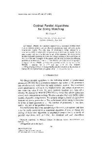
Figure 1: An example of the Data Distribution Management problem in d = 2 dimensions. Algorithm 1 Intersect-1D(x, y) return x.low ≤ y.high ∧ y.low ≤ x.high
In this section we define the DDM problem, and describe three matching algorithms that have been thoroughly investigated in the literature (brute-force, region-based and sortbased), in addition to one that has been introduced recently (interval-tree matching). Given two sets S = {S1 , . . . , Sn } and U = {U1 , . . . , Um } of d-dimensional rectangles with sides parallel to the axes (called subscription extents and update extents, respectively), the DDM problem consists of identifying all intersections between a subscription extent and an update extent. Formally, a DDM algorithm must return the list of all pairs (Si , Uj ) such that Si ∩ Uj 6= ∅, 1 ≤ i ≤ n, 1 ≤ j ≤ m. Figure 1 shows an instance of the DDM problem in d = 2 dimensions with three subscription extents {S1 , S2 , S3 } and two update extents {U1 , U2 }. There are four overlaps (intersections) between a subscription an update extent, namely (S1 , U1 ), (S2 , U2 ), (S3 , U1 ), and (S3 , U2 ). Note that S1 and S2 overlap, but this intersection is ignored since it involves subscription extents only. The time complexity of any DDM algorithm is outputsensitive, since it depends on the size of the output in addition to the size of the input. Therefore, every DDM algorithm that explicitly enumerates all the K intersections requires time Ω(K). Since there can be at most n × m intersections, the worst-case complexity of the DDM problem is O(n × m). One of the key steps of any DDM algorithm is testing whether two d-rectangles overlap. The special case d = 1 is quite simple, as it reduces to testing whether two closed intervals x = [x.low, x.high], y = [y.low, y.high] intersect; this can be done in constant time: x and y overlap if and only if x.low ≤ y.high ∧ y.low ≤ x.high (see Algorithm 1). The general case d > 1 can be reduced to the base case d = 1 by observing that two d-rectangles overlap if and only if all their projections along each dimension overlap. Therefore, we can invoke Algorithm 1 d times, and compute the logical “and” of the results. Using this property, an algorithm that enumerates all intersections among two sets of n and m
Algorithm 2 BruteForce-1D(S, U) 1: n ← |S|, m ← |U|, L ← ∅ 2: for i ← 1 to n do 3: for j ← 1 to m do 4: if Intersect-1D(Si , Uj ) then 5: L ← L ∪ (Si , Uj ) 6: return L
Figure 3: A set of intervals and the corresponding interval tree.
Figure 2: Grid-based matching in d = 2 dimensions. one-dimensional segments in time O (f (n, m)) can be readily extended to an O (d × f (n, m)) algorithm for reporting intersections among two sets of d-rectangles. For this reason, it is common practice in the DDM research community to focus on the simpler one-dimensional case.
3.1 Brute-Force Matching The simplest solution to the 1-dimensional segment intersection problem is the BF approach, also called RegionBased matching (Algorithm 2). The BF algorithm, as the name suggests, checks all n × m subscription-update pairs and inserts every intersection into a list L. Despite its simplicity, the BF algorithm is extremely inefficient since it requires time O(nm). However, it exhibits an embarrassingly parallel structure since the loop iterations (lines 2–5) are independent. This makes parallelization of the the BF algorithm trivial; when P processors are available, the amount of work performed by each processor is O (nm/P ).
3.2 Grid-Based Matching The Grid Based (GB) matching algorithm proposed by Boukerche and Dzermajko [5] improves over BF matching. GB works by partitioning the routing space into a regular mesh of d-dimensional cells. Each subscription or update extent is mapped to the grid cells it overlaps with. Events generated by an update extent Uj are sent to all subscription extents that share at least one cell with Uj . A filtering mechanism must then be applied to avoid delivering of spurious events. For example, in Figure 2 we see that S2 shares the hatched grid cells with U1 , but does not overlap with U1 . Hence, the GB matching algorithm would send notifications from U1 to S2 that will need to be filtered out. A simple filtering mechanism consists on the application of the BF algorithm to each grid cell. If the routing space is partitioned into G cells and all extents are evenly distributed, each cell will overlap with n/G subscription and m/G update extents on average. Therefore, the brute force
approach applied to each cell will require O(nm/G2 ) operations; since there are G cells, the overall worst-case complexity of GB matching is O(nm/G). Therefore, in the ideal case GB can decrease the matching complexity by a factor G with respect to BF. Unfortunately, when cells are small (and therefore G is large) each extent is mapped to a larger number of cells, which increases the computation time.
3.3 Interval-Tree Matching The Interval Tree Matching (ITM) algorithm [18] is based on the interval tree data structure that solves the matching problem in one dimension. An interval tree is a balanced search tree that stores a dynamic set of intervals, supporting insertions, deletions, and queries to get the list of segments intersecting a given interval q. Different implementations of interval trees are possible, depending on the structure of the underlying search tree; the implementation described in [18] is based on AVL trees [2]. Each node x of the AVL tree holds three fields: (i ) an interval x.in, represented by its lower and upper bounds; (ii ) the minimum lower bound x.minlower among all intervals stored at the subtree rooted at x; (iii ) the maximum upper bound x.maxupper among all intervals stored at the subtree rooted at x. Nodes are kept sorted according to the interval lower bounds. Figure 3 shows a set of intervals and the corresponding interval tree representation. Insertions and deletions are handled according to the normal rules for AVL trees, with the additional requirement that any update of the values of maxupper and minlower must be propagated up to the tree root. Since the height of an AVL tree is O(log n), insertions and deletions in the augmented data structure require O(log n) time in the worst case. The storage requirement is O(n). Function IntTree-Matching-1D (Algorithm 3) returns the list of intersections among the set S of subscription intervals and the set U of update intervals. This is done by first building an interval tree T containing all elements in S (line 12); then, for each update interval Uj ∈ U, the algorithm calls function Interval-Query(x, q) to identify all subscriptions that intersect Uj (lines 13–14). The function returns the list of intersections of the update interval q with the segments stored in the subtree rooted at x (T.root is the root of T ). Function Interval-Query performs a visit of the interval tree data structure, using the values of attributes x.minlower and x.maxupper of each node x to steer the visit out of the subtrees that would yield no matches.
Algorithm 3 Interval-Tree-Matching-1D(S, U) 1: function Interval-Query(x, q) 2: L←∅ 3: if x = null or x.maxupper < q.lower or x.minlower > q.upper then 4: return L 5: L ← Interval-Query(x.left, q) 6: if Intersect-1D(x.in, q) then 7: L ← L ∪ {(x.in, q)} 8: if q.upper ≥ x.in.lower then 9: L ← L ∪ Interval-Query(x.right, q) 10: return L 11: 12: 13: 14: 15:
n ← |S|, m ← |U|, L ← ∅ T ← create interval tree for S for j ← 1 to m do L ← L ∪ Interval-Query(T.root, Uj ) return L
Algorithm 4 Sort-Based-Matching-1D(S, U) 1: L ← ∅, T ← ∅ 2: for all extents x ∈ S ∪ U do 3: Insert x.lower and x.upper in T 4: Sort T in non-decreasing order 5: SubSet ← ∅, UpdSet ← ∅ 6: for all points t ∈ T in non-decreasing order do 7: if t belongs to subscription extent Si then 8: if t is the lower bound of Si then 9: SubSet ← SubSet ∪ {Si } 10: else 11: SubSet ← SubSet \ {Si } 12: for all x ∈ UpdSet do 13: L ← L ∪ {(Si , x)} 14: else ⊲ t belongs to update extent Uj 15: if t is the lower bound of Uj then 16: UpdSet ← UpdSet ∪ {Uj } 17: else 18: UpdSet ← UpdSet \ {Uj } 19: for all x ∈ SubSet do 20: L ← L ∪ {(x, Uj )} 21: return L
An interval tree can be created in time O(n log n); the total query time is O (min{mn, (K + 1) log n}), K ≤ nm being the number of intersections involving all subscription and all update intervals [18]. When executed on a shared-memory multiprocessor with P cores, the iterations of the for loop in Algorithm 3, lines 13–14 can be split across the cores, with the provision that updates to the result list L are serialized. The only remaining serial part is the construction of the interval tree; while concurrent balanced search trees have been proposed in the literature [19, 21] it is unclear whether they can be used as drop-in replacements.
3.4 Sort-Based Matching The Sort-based Matching algorithm [14, 23] is an efficient solution to the DDM problem. Algorithm 4 illustrates SBM in its basic form: given a set S of n subscription intervals, and a set U of m update intervals, the algorithm considers each of the 2 × (n + m) endpoints in non-decreasing order;
Figure 4: Value assigned by the SBM algorithm to the SubSet variable as the endpoints are swept from left to right. two sets SubSet and UpdSet are used to keep track of the active subscription and update intervals at every point t; we say that an interval is active at t if its lower endpoint has time ≤ t, and its upper endpoint has time > t. For example, Figure 4 shows the values of SubSet while the SBM sweeps through a set of subscription intervals (update intervals are handled in exactly the same way). When the upper bound of an interval is encountered, the list of intersections L is updated accordingly. Let N = n + m be the total number of endpoints; then, the SBM algorithm uses simple data structures and requires O (N log N ) time to sort the vector of endpoints, plus O(N ) time to scan the sorted vector. During the scan phase, O(K) time is spent in total to transfer the information from the sets SubSet and UpdSet to the intersection list L. The overall computational cost of SBM is O (N log N + K) (K is the number of intersections).
4. PARALLEL SORT-BASED MATCHING In this section we describe a parallel version of the SBM algorithm, using Algorithm 4 as the starting point. We have seen that SBM operates in two phases: first, the list T of endpoints is sorted; then, the sorted list is traversed to compute the values of the SubSet and UpdSet variables, from which the list of overlaps is derived. On a sharedmemory architecture with P processors, the sorting phase can be realized using a parallel sorting algorithm [9, 27]. The traversal of the sorted list of endpoints (Algorithm 4 lines 6–20) is, however, more challenging to execute in parallel. Ideally, we would like to split the list T into P segments of equal size T0 , . . . , TP −1 , and assign each segment to a processor. Unfortunately, this is made difficult by the loop-carried dependencies caused by the variables SubSet and UpdSet, whose values are modified at each iteration. Let us pretend that the scan phase can be parallelized somehow. Then, a parallel version of SBM would look like Algorithm 5 (line 6 will be explained shortly). The major difference between Algorithm 5 and its sequential counterpart is that the former uses two arrays SubSet[p] and UpdSet[p] instead of the scalar variables SubSet and UpdSet. This allows each core to operate on its private copy of the subscription and update sets, achieving the maximum level of parallelism. It is not difficult to see that Algorithm 5 is equivalent to the sequential SBM (i.e., they return the same result) if and only if SubSet[0..P − 1] and UpdSet[0..P − 1] are properly initialized. Specifically, SubSet[p] and UpdSet[p] must be initialized with the values that the sequential SBM algorithm assigns to SubSet and UpdSet right after the last endpoint of
Algorithm 5 Parallel-SBM-1D(S, U) 1: L ← ∅, T ← ∅ 2: for all extents x ∈ S ∪ U in parallel do 3: Insert x.lower and x.upper in T 4: Sort T in parallel, in non-decreasing order 5: Split T into P segments T0 , . . . , TP −1 6: hInitialize SubSet[0..P − 1] and UpdSet[0..P − 1]i 7: for p ← 0 to P − 1 in parallel do 8: for all endpoints t ∈ Tp in non-decreasing order do 9: if t belongs to subscription extent Si then 10: if t is the lower bound of Si then 11: SubSet[p] ← SubSet[p] ∪ {Si } 12: else 13: SubSet[p] ← SubSet[p] \ {Si } 14: for all x ∈ UpdSet[p] do 15: Atomic L ← L ∪ {(Si , x)} 16: else ⊲ t belongs to update extent Uj 17: if t is the lower bound of Uj then 18: UpdSet[p] ← UpdSet[p] ∪ {Uj } 19: else 20: UpdSet[p] ← UpdSet[p] \ {Uj } 21: for all x ∈ SubSet[p] do 22: Atomic L ← L ∪ {(x, Uj )} 23: return L
Tp−1 is processed, p = 1, . . . , P − 1; SubSet[0] and UpdSet[0] must be initialized to the empty set. It turns out that the content of the arrays SubSet[0..P −1] and UpdSet[0..P −1] can be computed efficiently using a prefix computation (also called scan or prefix-sum). To make this paper self-contained, we provide details on prefix computations before illustrating the missing part of the parallel SBM algorithm.
Prefix computations. A prefix computation consists of a sequence of N > 0 data items x0 , . . . , xN−1 and an associative operator ⊕. There are two types of prefix computations: the inclusive scan operation produces a new sequence of N data items y0 , . . . , yN−1 such that: y0 = x 0 y1 = y0 ⊕ x 1 y2 = y1 ⊕ x 2
= x0 ⊕ x1 = x0 ⊕ x1 ⊕ x2
.. . yN−1 = yN−2 ⊕ xN−1 = x0 ⊕ x1 ⊕ . . . ⊕ xN−1 while the exclusive scan operation produces the sequence z0 , z1 , . . . zN−1 such that: z0 = 0 z1 = z0 ⊕ x 0 z2 = z1 ⊕ x 1
= x0 = x0 ⊕ x1
.. . zN−1 = zN−2 ⊕ xN−2 = x0 ⊕ x1 ⊕ . . . ⊕ xN−2 where 0 is the neutral element of operator ⊕, i.e., 0 ⊕ x = x. Blelloch [4] showed that the prefix sums of N items can
Figure 5: Parallel prefix sum computation.
be computed in time O(N/P + log P ) using P < N processors on a shared-memory multiprocessor by organizing the computation as a tree. The O(N/P + log P ) time is optimal when N/P > log P . In our algorithm we use a simpler twolevel mechanism that achieves running time O(N/P + P ), which is still optimal when N/P > P . This is usually the case, since the current generation of CPUs have a small number of cores (e.g., P ≤ 72 for the Intel Xeon Phi) and the number of extents N is usually very large. We remark that the parallel SBM algorithm can be readily implemented with the tree-structured reduction operation, and therefore will still be competitive on future generations of processors with a higher number of cores. Figure 5 illustrates an example of parallel (inclusive) scan with P = 4 processors, assuming that the ⊕ operator is the numeric addition. The computation involves two parallel steps, and one serial step which is executed by a single processor that we call the master. 1 The input sequence is splitted across the processors, and each processor computes the prefix sum of the elements in its portion. 2 The master computes the prefix sum of the P last local sums. 3 The master scatters the first (P − 1) computed values (prefix sums of the last local sums) to the last (P − 1) processors. Each processor, except the first one, adds (more precisely, applies the ⊕ operator) the received value to the prefix sums from step , 1 producing a portion of the output sequence. Steps 2 is exe3 require time O(N/P ), while step 1 and cuted by the master only in time O(P ), yielding a total cost of O(N/P + P ).
Parallel Sort Matching. We are now ready to complete the description of the parallel SBM algorithm by showing how to fill the arrays SubSet[p] and UpdSet[p] in parallel. To better illustrate the steps involved, we refer to the example in Figure 6. In the figure, we consider subscription extents only, since the procedure for update extents is the same. The sorted list of endpoints T is evenly split into P segments T0 , . . . , TP −1 . Processor p scans the endpoints t ∈ Tp in non-decreasing order, updating four auxiliary variables
Figure 6: Parallel prefix computation for the SBM algorithm. Algorithm 6 hInitialize SubSet[0..P−1] and UpdSet[0..P−1]i ⊲ Executed by all cores in parallel 1: for p ← 0 to P − 1 in parallel do 2: Sadd[p] ← ∅, Sdel[p] ← ∅, Uadd[p] ← ∅, Udel[p] ← ∅ 3: for all points t ∈ Tp in non-decreasing order do 4: if t belongs to subscription extent Si then 5: if t is the lower bound of Si then 6: Sadd[p] ← Sadd[p] ∪ {Si } 7: else if Si ∈ Sadd[p] then 8: Sadd[p] ← Sadd[p] \ {Si } 9: else 10: Sdel[p] ← Sdel[p] ∪ {Si } 11: else ⊲ t belongs to update extent Uj 12: if t is the lower bound of Uj then 13: Uadd[p] ← Uadd[p] ∪ {Uj } 14: else if Uj ∈ Uadd[p] then 15: Uadd[p] ← Uadd[p] \ {Uj } 16: else 17: Udel[p] ← Udel[p] ∪ {Uj } ⊲ Executed by the master only 18: SubSet[0] ← ∅, UpdSet[0] ← ∅ 19: for p ← 1 to P − 1 do 20: SubSet[p] ← SubSet[p − 1] ∪ Sadd[p − 1] \ Sdel[p − 1] 21: UpdSet[p] ← UpdSet[p − 1] ∪ Uadd[p − 1] \ Udel[p − 1]
Sadd[p], Sdel[p], Uadd[p], and Udel[p]. Informally, Sadd[p] and Sdel[p] (resp. Uadd[p] and Udel[p]) contain the endpoints that the sequential SBM algorithm would add/remove from SubSet (resp. UpdSet) while scanning the endpoints belonging to segment Tp . More formally, at the end of each local scan the following invariants hold: 1. Sadd[p] (resp. Uadd[p]) contains the subscription (resp. update) intervals whose lower endpoint belongs to Tp , and whose upper endpoint does not belong to Tp ; 2. Sdel[p] (resp. Udel[p]) contains the subscription (resp.
update) intervals whose upper endpoint belongs to Tp , and whose lower endpoint does not belong to Tp . This step is realized by lines 1–17 of Algorithm 6, and its effects are shown in Figure 6 . 1 The figure reports the values of Sadd[p] and Sdel[p] after each endpoint has been processed; the algorithm does not store every intermediate value, since only the last ones (within thick boxes) will be needed by the next step. Once all Sadd[p] and Sdel[p] are available, the next step is executed by the master and consists of computing the values of SubSet[p] and UpdSet[p], p = 0, . . . , P −1. Recall from the discussion above that SubSet[p] (resp. UpdSet[p]) is the set of active subscription (resp. update) intervals that would be identified by the sequential SBM algorithm right after the end of segment T0 ∪ . . . ∪ Tp−1 . The values of SubSet[p] and SubSet[p] are related to Sadd[p], Sdel[p], Uadd[p] and Udel[p] as follows: ( ∅ if p = 0 SubSet[p] = SubSet[p − 1] ∪ Sadd[p] \ Sdel[p] if p > 0 ( ∅ if p = 0 UpdSet[p] = UpdSet[p − 1] ∪ Uadd[p] \ Udel[p] if p > 0 Intuitively, the set of active intervals at the end of Tp can be computed from those active at the end of Tp−1 , plus the intervals that became active in Tp , minus those that ceased to be active in Tp . Lines 18–21 of Algorithm 6 take care of this computation; see also Figure 6 2 for an example. Once the initial values of SubSet[p] and UpdSet[p] have been computed, Algorithm 5 can be resumed to identify the list of overlaps.
Asymptotic Analysis. We now analyze the asymptotic cost of parallel SBM. Algorithm 5 consists of three phases: 1. Fill the array of endpoints T , and sort T in non-decreasing order; if P processors are available, this step requires
total time O (N log N/P ), where N is the total number of subscription and update extents, using a suitable sorting algorithm such as parallel merge sort [9]. 2. Compute the initial values of SubSet[p] and UpdSet[p], for each p = 0, . . . , P −1; this phase requires O (N/P + P ) steps using the two-level scan shown on Algorithm 6; the time can be further reduced to O (N/P + log P ) steps using a tree-structured reduction [4]. 3. Perform the final local scans. Each scan can be completed in O(N/P ) steps. Note, however, that phases 2 and 3 require the manipulation of data structures to hold sets of endpoints, supporting insertions and removals of single elements and whole sets. Therefore, a single step of the algorithm has a non-constant time complexity that depends on the actual implementation of sets and the number of elements they contain. Furthermore, during phase 3 total time O(K) is spend cumulatively by all processors to push all K intersections into the result list L.
5.
EXPERIMENTAL EVALUATION
In this section we evaluate the performance and scalability of parallel SBM with respect to parallel versions of the BF and ITM algorithms. BF and ITM are considered because both exhibit an embarrassingly parallel structure, and ITM has already been shown to be more computationally efficient than BF [18]. In the present study we do not consider the GB algorithm: while it can be very fast and contains easily exploitable parallelism, its efficiency depends on the grid size G that should either be judiciously selected, or adaptively defined by means of non-trivial heuristics [6]. Therefore, to reduce the number of degrees of freedom we restrict our study to algorithms that have no tunable parameters, postponing a more complete study to a forthcoming paper. To foster the reproducibility of our experiments, all the source code used in this performance evaluation, and the raw data obtained in the experiments execution, are freely available on the Web1 . The BF and ITM algorithms have been implemented in C, and the parallel SBM algorithm has been implemented in C++. We used the GNU C Compiler (GCC) version 4.8.4 with the -O3 -fopenmp -D_GLIBCXX_PARALLEL flags to turn on optimization and to enable parallel constructs at the compiler and library levels. Specifically, the -fopenmp flag allows the compiler to process OpenMP directives in the source code [10]. OpenMP is an open interface supporting shared memory parallelism in the C, C++ and FORTRAN programming languages. OpenMP allows the programmer to label specific sections of the source code as parallel regions; the compiler takes care of dispatching portions of these regions to separate threads, that the Operating System (OS) can schedule on separate processors or cores. In the C/C++ languages, OpenMP directives are specified using #pragma compiler hints. The OpenMP standard also defines a set of library functions that can be called by the programmer to query and control the execution environment programmatically. Both the BF and ITM algorithms required a single omp parallel for directive to parallelize their inner loop. The par1
http://pads.cs.unibo.it
allel SBM algorithm was more complex, and its implementation benefited from the use of some of the data structures and algorithms provided by the C++ Standard Template Library (STL) [26]. Specifically, to sort the endpoints we used the parallel std::sort function provided by the STL extensions for parallelism [8]. Indeed, the GNU STL provides several parallel sort algorithms (multiway mergesort and quicksort with various splitting heuristics) that are automatically selected at compile time when the -D_GLIBCXX_PARALLEL compiler flag is given. The remaining part of the SBM algorithm has been parallelized using explicit OpenMP directives. The Sort-based Matching (SBM) algorithm requires a suitable data structure to store the sets of endpoints SubSet and UpdSet (see Algorithms 5 and 6). Parallel SBM puts a higher strain on this data structure with respect to its sequential counterpart, since it requires efficient support for unions and differences between sets, in addition to insertions and deletions of single elements. We have experimented with three implementations for sets: (i ) bit vectors based on the std::vector STL container (note that std::bitset can not be used, since it requires the set size to be known at compile time); (ii ) an ad-hoc implementation of bit vectors based on raw memory manipulation; (iii ) the std::set container, which in the case of the GNU STL is based on Red-Black trees [3]. The latter turned out to be the most efficient, so the performance results reported in this section refer to the std::set container.
CPU Clock frequency Processors Total cores HyperThreading RAM L3 cache size
solaris
titan
Intel Xeon E5-2640 2.00 GHz 2 16 Yes 128 GB 20480 KB
Intel Core i7-5820K 3.30 GHz 1 6 Yes 64 GB 15360 KB
Table 1: Hardware specifications of the machines used for the experimental evaluation.
Experimental setup. The experiments have been carried out on two different machines, called solaris and titan, both running the 64 bit version of the Ubuntu 14.04.05 LTS OS. The hardware specifications are reported in Table 1: solaris has two Intel Xeon processors with 8 cores each (16 cores total); titan has a single Intel Core i7 processor with 6 cores. Both types of processors employ the HT technology [17]. In HT-enabled CPUs some functional components are duplicated, but there is a single main execution unit for physical core. From the point of view of the OS, HT provides two “logical” processors for each physical core. Studies from Intel and others have shown that HT contributes a performance boost between 16–28% [17]. This means that when two processes are executed on the same core, the processes compete for the shared hardware resources resulting is lower efficiency. When running an OpenMP program it is possible to choose the number P of threads to use, either in the source code or through the OMP_NUM_THREADS environment variable. In
(a) Wall-clock time
(b) Speedup
Figure 7: Wall clock time and speedup of parallel {BF, ITM, SBM} with N = 106 extents and overlapping degree α = 100. Dashed lines indicate the region where the number of OpenMP threads exceeds the number of CPU cores, and therefore HT comes into play. our experiments below, P never exceeds twice the number of physical cores provided by the processor, so that the OS will be able to assign each thread to a separate (logical) core. Unless configured differently, the Linux scheduler tries to spread processes to different cores as far as possible; only when there are more runnable processes than cores does HT come into effect. For better comparability of our results with those reported in the literature we consider d = 1 dimensions and use the methodology and parameters described in [23]. The first parameter is the total number of extents N , that includes n = N/2 subscription and m = N/2 update extents. All extents are randomly placed on a segment of total length L = 106 and have the same length l. The segment length is defined in such a way that a given overlapping degree α is obtained, where α=
P
area of extents N ×l = area of the routing space L
Therefore, given α and N , the length l of each segment is set to l = αL/N . The overlapping degree is an indirect measure of the total number of intersections among subscription and update extents. While the cost of BF and SBM is not affected by the number of intersections, this is not the case for ITM, as will be shown below. We considered the same values for α as in [23], namely α ∈ {0.01, 1, 100}. Finally, each measure is the average of 30 independent runs to get statistically valid results. Our implementations do not explicitly store the list of intersections, but only count them. We did so to ensure that the algorithms run time is not affected by the choice of the data structure used to store the intersections.
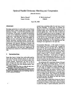
Wall clock time. The first performance metric we analyze is the Wall Clock Time (WCT) of the algorithms. Figure 7(a) shows the WCT for the parallel versions of BF, ITM and SBM as a function of the number P of OpenMP threads used, given N = 106 extents and overlapping degree α = 100. Dashed lines indicate when P exceeds the number
of CPU cores. With those parameters, the parallel BF algorithm is about three orders of magnitude slower than SBM on both the titan and solaris machine. For larger values of N the gap widens further, since BF is asymptotically slower than the other two algorithms. Indeed, the computational cost of BF grows quadratically with the number of extents (see Section 3), while that of SBM and ITM grows only polylogarithmically. ITM performs better than BF, but worse than SBM. In Figure 8 we study how the WCT of the parallel ITM and SBM algorithms depend on the number of extents N and the overlapping degree α. The measures were taken on both machines (solaris and titan) with as many OpenMP threads as physical cores. Figure 8(a) shows that the WCT grows polylogarithmically with N for both ITM and SBM, confirming the asymptotic analysis in Section 4; however, the parallel SBM algorithm is faster than ITM on both machines, suggesting that its asymptotic cost has smaller constants and terms of lower order. In Figure 8(b) we report the WCT as a function of α, for a fixed N = 108 . We observe that, unlike ITM, the execution time of SBM is essentially independent from the overlapping degree.
Speedup. The relative speedup measures the increase in speed that a parallel program achieves when more processors are employed to solve a problem of the same size. This metric can be computed from the WCT as follows. Let T (N, P ) be the WCT required to process an input of size N using P processes (OpenMP threads). Then, for a given N , the relative speedup SN (P ) is defined as SN (P ) = T (N, 1)/T (N, P ). Ideally, the maximum value of SN (P ) is P , which means that solving a problem with P processors requires 1/P the time needed by a single processor. In practice, however, several factors limit the speedup, such as the presence of serial regions in the parallel program, uneven load distribution, scheduling overhead, and heterogeneity in the execution hardware.
(a)
(b)
Figure 8: Wall clock time of parallel ITM and SBM as a function of the number of extents N (a) and overlapping degree α (b) (note the logarithmic horizontal scale). Figure 7(b) shows the speedups of the parallel versions of BF, ITM and SBM as a function of the number of OpenMP threads P ; the speedups have been computed using the wall clock times of Figure 7(a). Line colors denote the algorithm, while the shape of the data points denote the host where the tests have been executed (square = solaris, circle = titan). Dashed lines indicate data points where P exceeds the number of physical processor cores available on that machine. The BF algorithm, despite being the less efficient, is the most scalable. This can be attributed to its embarrassingly parallel structure and lack of any serial part. SBM, on the other hand, is the most efficient but the less scalable. Interestingly, with equal number of OpenMP threads, SBM and ITM scale better on the i7 machine (titan) than on the Xeon machine (solaris), while BF seems unaffected by the processor type. SBM achieves a 2.6× speedup with 16 OpenMP threads on the dual Xeon machine, and a 2.9× speedup with 6 OpenMP threads on the Core i7 machine. When all “virtual” cores are used, the speedup grows to 3.6× on the Xeon machine and 4.1× on the i7. The effect of HT (dashed lines) is clearly visible in Figure 7(b). The speedup degrades when P exceeds the number of cores, as can be seen from the different slopes for BF on titan. When HT kicks in, load unbalance arises due to contention of the shared control units of the processor cores, and this limits the scalability. The bizarre behavior of BF on solaris around P = 24 (the speedup drops and then raises again) is likely caused by OpenMP Non Uniform Memory Access (NUMA) scheduling issues [7]. Considering the high wall clock time of the BF algorithm, we do not address this issue in this paper. The speedup of SBM improves slightly if we increase the work performed by the algorithm. Figure 9 shows the speedup of parallel ITM and SBM with N = 108 extents and overlapping degree α = 100 (in this scenario BF takes so long that it has been omitted). The SBM algorithm behaves better, especially on the dual socket Xeon machine, achieving a 4.5× speedup with 16 OpenMP threads, and 7× speedup with 32 threads. On the Core i7 machine the speedup is 3.6× with 6 OpenMP threads (one per core), and 5.1× with 12 threads (two per core).
Figure 9: Speedup of parallel {ITM, SBM} with N = 108 extents, overlapping degree α = 100.
Scaling Efficiency. The scaling efficiency measures how well a parallel application exploits the available computational resources. Two formulation of scaling efficiency are given in the literature: strong scaling and weak scaling. Given an input of size N and P processors, the strong scaling efficiency EN,strong (P ) and weak scaling efficiency EN,weak (P ) are defined as: T (N, 1) SN (P ) = P × T (N, P ) P T (N, 1) EN,weak (P ) = T (P × N, P )
EN,strong (P ) =
Scaling efficiencies are real numbers in the range [0, 1]. An efficiency of, say, 0.8 indicates that the application spends 80% of the time doing actual work, the rest being communication and synchronization overhead. Therefore, higher efficiencies denote better scaling behavior. Strong scaling measures how well a parallel application exploits the processors, assuming constant total problem size. Weak scaling
(a) Strong scaling
(b) Weak scaling
Figure 10: Strong and weak scaling behavior of parallel ITM and SBM, overlapping degree α = 100. measures how well the application exploits the processors under constant per-processor work. Strong and weak scaling are investigated in Figure 10, assuming overlapping degree α = 100. We observe that both efficiencies sharply drop when going from P = 1 to P = 2 and P = 4 OpenMP threads. Looking at the strong scaling behavior of SBM and ITM (Figure 10(a)), SBM scales better than ITM on the Intel i7 machine. On the other hand, ITM is more efficient than SBM on the Xeon machine up to P = 8 OpenMP threads; after that, SBM becomes more efficient. Weak scaling (Figure 10(b)) shows a similar behavior: SBM scales consistently better than ITM on titan, while on solaris ITM is better than SBM up to P = 6 OpenMP threads. Figure 10 confirms that the OpenMP SBM implementation exhibits efficiency issues. The reason is still being investigated, since it is unclear whether NUMA memory issues can explain this behavior.
In Figure 11(b) we study the RSS as a function of the number of OpenMP threads P . The RSS for BF and ITM grows very slowly with P , since they do not explicitly use additional per-thread variables; therefore, the marginal increase of RSS that we observe is due to the normal overhead of the OpenMP threading system. On the other hand, the RSS for the parallel SBM algorithm is strongly influenced by the number of threads, although the variability is so high that it is not possible to observe a smooth correlation (despite each data point being computed over multiple runs). Such variability is likely caused by memory fragmentation induced by the STL data structures used by the algorithm. In any case, the RSS for SBM shows only a threefold increase when moving fro P = 2 to P = 16 OpenMP threads; we can therefore postulate that the RSS will not become a bottleneck for any reasonable number of OpenMP threads that are used.
Memory Usage. We conclude our experimental evaluation
6. CONCLUSIONS AND FUTURE WORKS
with an assessment of the memory usage of the parallel BF, ITM and SBM algorithms. Figure 11 shows the peak Resident Set Size (RSS) of the three algorithms as a function of the number of extents and OpenMP threads; the data have been collected on the Xeon machine solaris. The RSS is the portion of a process memory that is kept in RAM. Care has been taken to ensure that all experiments reported in this section fit comfortably in the main memory of the available machines, so that the RSS represents an actual upper bound of the amount of memory required by the algorithms. Note that the data reported in Figure 11 includes the code for the test driver and the input arrays of intervals. Figure 11(a) shows that the resident set size grows linearly with the number of extents N . BF has the smaller memory footprint, since it requires a tiny bounded amount of additional memory for a few local variables; SBM uses more memory since it allocates larger data structures, namely the list of endpoints to be sorted, and a few arrays of sets. SBM requires approximately 7 GB of memory to process N = 108 intervals, about three times the amount of memory required by BF.
In this paper we described a parallel version of the SBM algorithms for solving the d-rectangle intersection problem for Data Distribution Management. Our algorithm is targeted at shared-memory multicore architectures that constitute the vast majority of current processors. We have implemented the parallel SBM algorithm in C++ with OpenMP directives. Performance measurement shows a 2.6× speedup with 16 OpenMP threads on a dual Intel Xeon processor, and a 2.9× speedup with 6 threads on an Intel Core i7 processor. The memory usage of parallel SBM grows linearly with the number of extents N ; memory usage also depends on the number of OpenMP threads used. In any case, SBM uses about 7 GB of memory to handle 100 millions of extents, making it attractive for large scenarios. We are currently extending the present work in two directions. First, we are studying how the choice of parallel sorting algorithm and of dynamic set data structure influence the scalability of parallel SBM. Indeed, while the results presented in Section 5 are encouraging, scalability is lower than what asymptotic analysis predicts, suggesting the presence of bottlenecks in the implementation that should be identified and removed. Scheduling issues and NUMA
(a)
(b)
Figure 11: Memory usage (peak resident set size, VmHWM) of parallel {BF, ITM, SBM} with an increasing number of extents (a) or threads (b), overlapping degree α = 100. memory conflicts are suspected to play a significant role in the loss of efficiency that we observe on the dual-socket test machine. Second, we are extending the SBM algorithm to solve the dynamic DDM matching problem, where extents can be moved or resized dynamically. This problem has already been investigated in the context of serial SBM [20], so it is important to assess if and how it can be solved in a parallel environment.
Notation S U n m N K α P
Subscription set S = {S1 , . . . , Sn } Update set U = {U1 , . . . , Um } Number of subscription extents Number of update extents N. of subscription and update extents (N = n + m) Number of intersections, 0 ≤ K ≤ n × m Overlapping degree (α > 0) Number of processors/OpenMP threads
Acronyms BF
Brute Force
DDM
Data Distribution Management
GB
Grid Based
HLA
High Level Architecture
HT
Hyper-Threading
ITM
Interval Tree Matching
NUMA Non Uniform Memory Access OS
Operating System
RSS
Resident Set Size
SBM
Sort-based Matching
STL
Standard Template Library
WCT
Wall Clock Time
7. REFERENCES [1] IEEE Standard for Modeling and Simulation (M&S) High Level Architecture (HLA)–Framework and Rules. IEEE Std 1516-2010 (Rev. of IEEE Std 1516-2000), 2010. [2] G. Adelson-Velskii and E. M. Landis. An Algorithm for the Organization of Information. Doklady Akademii Nauk USSR, 146(2):263–266, 1962. [3] R. Bayer. Symmetric binary B-Trees: Data structure and maintenance algorithms. Acta Informatica, 1(4):290–306, 1972. [4] G. E. Blelloch. Scans as primitive parallel operations. IEEE Transactions on Computers, 38(11):1526–1538, Nov 1989. [5] A. Boukerche and C. Dzermajko. Performance comparison of data distribution management strategies. In Proc. 5th IEEE Int. Workshop on Distributed Simulation and Real-Time Applications, DS-RT ’01, pages 67–, Washington, DC, USA, 2001. IEEE Computer Society. [6] A. Boukerche and A. Roy. Dynamic grid-based approach to data distribution management. Journal of Parallel and Distributed Computing, 62(3):366–392, 2002. [7] F. Broquedis, F. Diakhat´e, S. Thibault, O. Aumage, R. Namyst, and P.-A. Wacrenier. Scheduling dynamic openmp applications over multicore architectures. In R. Eigenmann and B. R. de Supinski, editors, OpenMP in a New Era of Parallelism: 4th International Workshop, IWOMP 2008 West Lafayette, IN, USA, May 12-14, 2008 Proceedings, pages 170–180, Berlin, Heidelberg, 2008. Springer Berlin Heidelberg. [8] Programming languages – technical specification for C++ extensions for parallelism. ISO/IEC TS 19570:2015, 2015. [9] R. Cole. Parallel merge sort. SIAM Journal on Computing, 17(4):770–785, 1988. [10] L. Dagum and R. Menon. OpenMP: An industry-standard API for shared-memory programming. IEEE Comput. Sci. Eng., 5:46–55,
January 1998. [11] G. D’Angelo and M. Marzolla. New trends in parallel and distributed simulation: From many-cores to cloud computing. Simulation Modelling Practice and Theory, 49:320–335, 2014. [12] F. Devai and L. Neumann. A rectangle-intersection algorithm with limited resource requirements. In Proc. 10th IEEE Int. Conf. on Computer and Information Technology, CIT ’10, pages 2335–2340, Washington, DC, USA, 2010. IEEE Computer Society. [13] A. Guttman. R-trees: a dynamic index structure for spatial searching. SIGMOD Rec., 14(2):47–57, June 1984. [14] Y. Jun, C. Raczy, and G. Tan. Evaluation of a sort-based matching algorithm for DDM. In Proceedings 16th Workshop on Parallel and Distributed Simulation, pages 62–69, 2002. [15] E. S. Liu and G. K. Theodoropoulos. An analysis of parallel interest matching algorithms in distributed virtual environments. In 2013 Winter Simulations Conference (WSC), pages 2889–2901, Dec 2013. [16] Y. Liu, H. Sun, W. Fan, and T. Xiao. A parallel matching algorithm based on order relation for hla data distribution management. International Journal of Modeling, Simulation, and Scientific Computing, 06(02):1540002, 2015. [17] D. T. Marr, F. Binns, D. L. Hill, G. Hinton, D. A. Koufaty, A. J. Miller, and M. Upton. Hyper-Threading Technology Architecture and Microarchitecture. Intel Technology Journal, 6(1), Feb. 2002. [18] M. Marzolla, G. D’Angelo, and M. Mandrioli. A parallel data distribution management algorithm. In 2013 IEEE/ACM 17th International Symposium on Distributed Simulation and Real Time Applications (DS-RT), pages 145–152, Oct 2013. [19] M. Medidi and N. Deo. Parallel Dictionaries Using AVL Trees. Journal of Parallel and Distributed Computing, 49(1):146–155, 1998. [20] K. Pan, S. J. Turner, W. Cai, and Z. Li. A dynamic sort-based DDM matching algorithm for HLA applications. ACM Trans. Model. Comput. Simul., 21(3):17:1–17:17, Feb. 2011. [21] H. Park and K. Park. Parallel algorithms for red-black trees. Theor. Computer Science, 262(1):415–435, 2001. [22] M. D. Petty and A. Mukherjee. Experimental comparison of d-rectangle intersection algorithms applied to HLA data distribution. In Proceedings of the 1997 Distributed Simulation Symposium, pages 13–26, 1997. [23] C. Raczy, G. Tan, and J. Yu. A sort-based DDM matching algorithm for HLA. ACM Trans. Model. Comput. Simul., 15(1):14–38, Jan. 2005. [24] D. Rao, X. Hu, and L. Wu. Performance analysis of parallel data distribution management in large-scale battlefield simulation. In Proceedings of 2013 3rd International Conference on Computer Science and Network Technology, pages 134–138, Oct 2013. [25] J. Rosenberg. Geographical data structures compared: A study of data structures supporting region queries. Computer-Aided Design of Integrated Circuits and Systems, IEEE Transactions on, 4(1):53–67, 1985.
[26] B. Stroustrup. The C++ Programming Language, 4th Edition. Addison-Wesley, 2013. [27] M. Wheat and D. Evans. An efficient parallel sorting algorithm for shared memory multiprocessors. Parallel Computing, 18(1):91–102, 1992.