Jun 2, 2016 - MS] 2 Jun 2016. Parallel ... The support of Department of Chemical and Petroleum Engineering, University of. Calgary and ..... conditioned iterative methods on the GPU, NVIDIA Technical Report, June 2011. 14. X.-C. Cai and ...
Parallel Triangular Solvers on GPU Zhangxin Chen ⋆ , Hui Liu, and Bo Yang
arXiv:1606.00541v1 [cs.MS] 2 Jun 2016
University of Calgary 2500 University Dr NW, Calgary, AB, Canada, T2N 1N4 {zhachen,hui.j.liu,yang6}@ucalgary.ca
Abstract. In this paper, we investigate GPU based parallel triangular solvers systematically. The parallel triangular solvers are fundamental to incomplete LU factorization family preconditioners and algebraic multigrid solvers. We develop a new matrix format suitable for GPU devices. Parallel lower triangular solvers and upper triangular solvers are developed for this new data structure. With these solvers, ILU preconditioners and domain decomposition preconditioners are developed. Numerical results show that we can speed triangular solvers around seven times faster. Keywords: Triangular solver, GPU, parallel, linear system
1
Introduction
In many scientific applications, we need to solve lower triangular problems and upper triangular problems, such as Incomplete LU (ILU) preconditioners, domain decomposition preconditioners and Gauss-Seidel smoothers for algebraic multigrid solvers [1,2]. The algorithms for these problems are serial in nature and difficult to parallelize on parallel platforms. GPU is one of these parallel devices, which is powerful in float point calculation and is over 10 times faster than latest CPU. Recently, GPU has been popular in various numerical scientific applications. It is efficient for vector operations. Researchers have developed linear solvers for GPU devices [3,4,7,8,11]. However, the development of efficient parallel triangular solvers for GPU is still challenging [11,12,13]. Klie et al. (2011) investigated a triangular solver [7]. They developed a level schedule method and a speedup of two was obtained. Naumov (2011) from the NVIDIA company also developed parallel triangular solvers [13]. He developed new parallel triangular solvers based on a graph analysis. The average speedup was also around two. In this paper, we introduce our work on speeding triangular solvers. A new matrix format, HEC (Hybrid ELL and CSR), is developed. A HEC matrix includes two matrices, an ELL matrix and a CSR matrix. The ELL part is in column-major order and is designed the way to increase the effective bandwidth ⋆
The support of Department of Chemical and Petroleum Engineering, University of Calgary and Reservoir Simulation Group is gratefully acknowledged. The research is partly supported by NSERC/AIEE/Foundation CMG and AITF Chairs.
2
Parallel Triangular Solvers on GPU
of NVIDIA GPU. For the CSR matrix, each row contains at least one non-zero element. This design of the CSR part reduces the complexity of the solution of triangular systems. In addition, parallel algorithms for solving the triangular systems are developed. The algorithms are motivated by the level schedule method described in [2]. Our parallel triangular solvers can be sped up to seven times faster. Based on these modified algorithms, ILU(k), ILUT and domain decomposition (Restricted Additive Schwarz) preconditioners are developed. Numerical experiments are performed. These experiments show that we can speed linear solvers around ten times faster. The layout is as follows. In §2, a new matrix format and algorithms for lower triangular problems and upper triangular problems are introduced. In §3, parallel triangular solvers are employed to develop ILU preconditioners and domain decomposition preconditioners. In §4, numerical tests are performed. At the end, conclusions are presented.
2
Parallel Triangular Solvers
For the most commonly used preconditioner ILU, the following triangular systems need to be solved: LU x = b ⇔ Ly = b, U x = y,
(1)
where L and U are a lower triangular matrix and an upper triangular matrix, respectively, b is the right-hand side vector, x is the unknown to be solved for, and y is the intermediate unknown. The lower triangular problem, Ly = b, is solved first, and then, by solving the upper triangular problem, U x = y, we can obtain the result x. In this paper, we always assume that each row of L and U is sorted in ascending order according to their column indices. 2.1
Matrix format
The matrix format we develop is denoted by HEC (Hybrid ELL and CSR) [5]. Its basic structure is demonstrated by Figure 1. An HEC matrix contains two submatrices: an ELL matrix, which was introduced in ELLPACK [6], and a CSR (Compressed Sparse Row) matrix. The ELL matrix has two submatrices, a column-indices matrix and a non-zeros matrix. The length of each row in these two matrices is the same. The ELL matrix is in column-major order and is aligned when being stored on GPU. Note that the data access pattern of global memory for NVIDIA Tesla GPU is coalesced [9] so the data access speed for the ELL matrix is high. A disadvantage of the ELL format is that it may waste memory if one row has too many non-zeros. In this paper, a CSR submatrix is added to overcome this problem. A CSR matrix contains three arrays, the first one for the offset of each row, the second one for column indices and the last one for non-zeros. For our HEC format matrix, we store the regular part of a given triangular matrix L in the ELL part and the irregular part in the CSR part. When we store the lower triangular matrix, each row of the CSR matrix has at least one element, which is the diagonal element in the triangular matrix L.
Parallel Triangular Solvers on GPU Aj
3
Ax
Ap
Aj
Ax
ELL
CSR
Fig. 1. HEC matrix format.
2.2
Parallel lower triangular solvers
In this section, we introduce our parallel lower triangular solver to solve Lx = b. The solver we develop is based on the level schedule method [2,8]. The idea is to group unknowns x(i) into different levels so that all unknowns within the same level can be computed simultaneously [2,8]. For the lower triangular problem, the level of x(i) is defined as l(i) = 1 + max l(j) j
f or all j such that Lij 6= 0, i = 1, 2, . . . , n,
(2)
where Lij is the (i, j)th entry of L, l(i) is zero initially and n is the number of rows. We define Si = {x(j) : l(j) = i}, which is the union of all unknowns that have the same level. Here we assume that each set Si is sorted in ascending order according to the indices of the unknowns belonging to Si . Define Ni the number of unknowns in set Si and nlev the number of levels. Now, a map m(i) can be defined as follows: m(i) =
k−1 X
Nj + pk (x(i)),
x(i) ∈ Sk ,
(3)
j=1
where pk (x(i)) is the position x(i) in the set Sk when x(i) belongs to Sk . With the help of the map, m(i), we can reorder the triangular matrix L to L′ , where Lij in L is transformed to L′m(i)m(j) in L′ . L′ is still a lower triangular matrix. From this map, we find that if x(i) is next to x(j) in some set Sk , the ith and jth rows of L are next to each other in L′ after reordering. It means that L is reordered level by level, which implies that memory access in matrix L′ is less irregular than that in matrix L. Therefore, L′ has higher performance compared to L when we solve a lower triangular problem. The whole algorithm is described in two steps, the preprocessing step and the solution step, respectively. The preprocessing step is described in Algorithm
4
Parallel Triangular Solvers on GPU
1. In this step, the level of each unknown is calculated first. According to these levels, a map between L and L′ can be set up according to equation (3). Then the matrix L is reordered. We should mention that L can be stored in any kind of matrix format. A general format is CSR. At the end, L′ is converted to the HEC format and as we discussed above each row of the CSR part has at least one element. Algorithm 1 Preprocessing lower triangular problem 1: 2: 3: 4:
Calculating the level of each unknown x(i) using equation (2). Calculating the map m(i) using equation (3). Reordering matrix L to L′ using map m(i). Converting L′ to the HEC format.
Algorithm 2 Parallel the lower triangular solver on GPU, Lx = b 1: 2: 3: 4: 5: 6: 7: 8: 9: 10: 11: 12: 13:
for i = 1: n do b′ (m(i)) = b(i); end for for i = 1 : nlev do start = level(i); end = level(i + 1) - 1; for j = start: end do solve the jth row; end for end for for i = 1: n do x(i) = x′ (m(i)); end for
⊲ Use one GPU kernel to deal with this loop
⊲ L′ x′ = b′
⊲ Use one GPU kernel to deal with this loop
⊲ Use one GPU kernel to deal with this loop
The second step is to solve the lower triangular problem. This step is described in Algorithm 2, where level(i) is the start row position of level i. First, the right-hand side b is permutated according to the map m(i) we computed. Then the triangular problem is solved level by level and the solution in the same level is simultaneous. Each thread is responsible for one row. At the end, the final solution is obtained by a permutation. To solve the upper triangular problem U x = b, we introduce the following transferring map: t(i) = n − i, where n is the number of rows in U . With this map, the upper triangular problem is transferred to a lower triangular problem, and the lower triangular solver is called to solve the problem.
Parallel Triangular Solvers on GPU
3
5
Preconditioners
The ILU factorization for a sparse matrix A computes a sparse lower triangular matrix L and a sparse upper triangular matrix U . If no fill-in is allowed, we obtain the so-called ILU(0) preconditioner. If fill-in is allowed, we obtain the ILU(k) preconditioner, where k is the fill-in level. Another method is ILUT(p,tol), which drops entries based on the numerical values tol of the fill-in elements and the maximal number p of non-zeros in each row [2,8]. The performance of parallel triangular solvers for ILU(k) and ILUT is dominated by original problems. In this paper, we implement block ILU(k) and block ILUT preconditioners. When the number of blocks is large enough, we will have sufficient parallel performance. If the matrix is not well partitioned and the number of blocks is too large, the effect of ILU(k) and ILUT will be weakened. When we partition a matrix, the graph library METIS [15] is employed. As we discussed above, the effect of ILU preconditioners is weakened if the number of blocks is too large. The domain decomposition preconditioner is implemented, which was developed by Cai et al. [14]. The domain decomposition preconditioner we implement is the so-called Restricted Additive Schwarz (RAS) method. Overlap is introduced, and, therefore, this preconditioner is not as sensitive as block ILU preconditioners. It can lead to good parallel performance and good preconditioning. In this paper, we treat the original matrix as an undirected graph and this graph is partitioned by METIS [15]. The subdomain can be extended according to the topology of the graph. Then each smaller problem can be solved by ILU(k) or ILUT. In this paper, we use ILU(0). Assume that the domain is decomposed into s subdomains, and we have s smaller problems, A1 , A2 , · · ·, and As . We do not solve these problems one by one but we treat them as one bigger problem: diag(A1 , A2 , · · · , As )x = b. Each Ai is factorized by the ILU method, where we have diag(L1 , L2 , · · · , Ls ) × diag(U1 , U2 , · · · , Us )x = L × U x = b.
(4)
Then equation (4) is solved by our triangular solvers.
4
Numerical Results
In this section, numerical experiments are presented, which are performed on our workstation with Intel Xeon X5570 CPUs and NVIDIA Tesla C2050/C2070 GPUs. The operating system is CentOS 6.2 X86 64 with CUDA Toolkit 4.1 and GCC 4.4. All CPU codes are compiled with -O2 option. The data type of a float point number is double. The linear solver is GMRES(20). BILU, BILUT and RAS denote the block ILU(0), block ILUT and Restricted Additive Schwarz preconditioners, respectively.
6
Parallel Triangular Solvers on GPU
Example 1. The matrix used in this example is from a three-dimensional Poisson equation. The dimension is 1,000,000 and the number of non-zeros is 6,940,000. The ILU preconditioners we use in this example are block ILU(0) and block ILUT(7, 0.1). The performance data is collected in Table 1.
Table 1. Performance of the matrix from the Poisson equation Pre
Blocks CPU (s) GPU (s) Speedup Pre CPU (s) Pre GPU (s) Speedup
BILU BILU BILU BILUT BILUT BILUT RAS RAS
16 128 512 16 128 512 256 2048
20.12 20.2 22.76 14.85 14.56 18.59 18.70 22.03
2.53 2.39 2.70 2.38 2.30 2.71 2.16 2.35
7.93 8.44 8.39 6.19 6.30 6.83 8.60 9.32
0.0197 0.0192 0.0188 0.0241 0.0239 0.0234 0.0306 0.0390
0.0057 0.0055 0.0052 0.010 0.011 0.010 0.0051 0.0056
3.46 3.46 3.61 2.27 2.25 2.24 5.94 6.92
For the block ILU(0), we can speed it over 3 times faster. When the number of blocks increases, our algorithm has better speedup. The whole solving part is sped around 8 times faster. BILUT is a special preconditioner, since it is obtained according to the values of L and U ; sometimes, the sparse patterns of L and U are more irregular than those in BILU. From Table 1, the speedups are a little lower compared to BILU. However, BILUT reflects the real data dependence, and its performance is better in general. This is demonstrated by Table 1. The CPU version BILUT always takes less time than the CPU BILU. But for the GPU versions, their performance is similar. The BILUT is sped around 2 times faster. The whole solving part is sped around 6 times faster. The RAS preconditioner is always stable. It also has better speedup than BILU and BILUT. The triangular solver is sped around 6 times faster and the average speedup is around 9. Example 2. Matrix atmosmodd is taken from the University of Florida sparse matrix collection [16] and is derived from a computational fluid dynamics (CFD) problem. The dimension of atmosmodd is 1,270,432 and it has 8,814,880 nonzeros. The ILU preconditioners we use in this example are block ILU(0) and block ILUT(7, 0.01). The performance data is collected in Table 2. The performance of BILU, BILUT and RAS is similar to that of the same preconditioners in Example 1. When BILU is applied, the triangular solvers are sped over 3 times faster and the speedup of the whole solving phase is about 7. Because of the irregular non-zero pattern of BILUT, the speedup of BILUT is around 2. The average speedup of the solving phase is about 6. The speedup increases when the number of blocks grows. RAS is as stable as in Example 1. The triangular solvers are sped around 6, and the average speedup of the solving phase is around 8.
Parallel Triangular Solvers on GPU
7
Table 2. Performance data of the matrix atmosmodd Pre
Blocks CPU (s) GPU (s) Speedup Pre CPU (s) Pre GPU (s) Speedup
BILU BILU BILU BILUT BILUT BILUT RAS RAS
16 128 512 16 128 512 256 2048
20.61 23.94 24.13 14.70 16.58 19.91 23.45 25.75
2.63 2.80 2.72 2.37 2.43 2.64 2.66 3.28
7.79 8.50 8.82 6.16 6.79 7.50 8.75 7.81
0.0248 0.0244 0.0241 0.028669 0.028380 0.027945 0.0428 0.0546
0.0072 0.0072 0.0070 0.0114 0.0100 0.0113 0.0072 0.0083
3.45 3.40 3.46 2.51 2.84 2.47 5.96 6.59
Example 3. A matrix from SPE10 is used [17]. SPE10 is a standard benchmark for the black oil simulator. The problem is highly heterogenous and it is designed the way so that it is hard to solve. The grid size for SPE10 is 60x220x85. The number of unknowns is 2,188,851 and the number of non-zeros is 29,915,573. The ILU preconditioners we use in this example are block ILU(0) and block ILUT(14, 0.01). The performance data is collected in Table 3.
Table 3. Performance of SPE10 Pre
Blocks CPU (s) GPU (s) Speedup Pre CPU (s) Pre GPU (s) Speedup
BILU BILU BILU BILUT BILUT BILUT RAS RAS
16 128 512 16 128 512 256 1024
92.80 86.22 92.82 32.00 42.51 47.44 106.61 110.36
12.78 12.05 12.87 7.17 7.82 8.80 14.36 16.36
7.25 7.14 7.20 4.46 5.42 5.37 7.41 6.73
0.0421 0.0423 0.0424 0.0645 0.0647 0.0645 0.100 0.124
0.0118 0.0119 0.0119 0.0747 0.0747 0.0747 0.0198 0.0242
3.54 3.56 3.56 0.86 0.86 0.86 5.07 5.11
From Table 3, we can speed the whole solving phase 6.2 times faster when ILU(0) is applied. The speedup increases if we increase the number of blocks. The average speedup of BILU is about 3 and the average speedup for the whole solving stage is about 7. In this example, BILUT is the best, which always takes the least running time. However, due to its irregular non-zero pattern, we fail to speed the triangular solvers. The RAS preconditioner is always stable, and the average speedup of RAS is about 5, while the average speedup of the solving phase is around 6.5.
5
Conclusions
We have developed a new matrix format and its corresponding triangular solvers. Based on them, the block ILU(k), block ILUT and Restricted Additive Schwarz
8
Parallel Triangular Solvers on GPU
preconditioners have been implemented. The block ILU(0) is sped over three times faster, the block ILUT is sped around 2 times, and the RAS preconditioner is sped up to 7 times faster. The latter preconditioner is very stable and it can be served as a general preconditioner for parallel platform.
References 1. R. Barrett, M. Berry, T. F. Chan, J. Demmel, J. Donato, J. Dongarra, V. Eijkhout, R. Pozo, C. Romine and H. Van der Vorst , Templates for the solution of linear systems: building blocks for iterative methods, 2nd Edition, SIAM, 1994. 2. Yousef Saad, Iterative methods for sparse linear systems (2nd edition), SIAM, 2003. 3. Nathan Bell and Michael Garland, Efficient sparse matrix-vector multiplication on CUDA, NVIDIA Technical Report, NVR-2008-004, NVIDIA Corporation, 2008. 4. Nathan Bell and Michael Garland, Implementing sparse matrix-vector multiplication on throughput-oriented processors, Proc. Supercomputing, November 2009, pp. 1-11. 5. Hui Liu, Song Yu, Zhangxin Chen, Ben Hsieh and Lei Shao, Sparse matrix-vector multiplication on Nvidia GPU, International Journal of Numerical Analysis & Modeling, 3(2), 2012, pp. 185-191. 6. R. Grimes, D. Kincaid, and D. Young, ITPACK 2.0 User’s Guide, Technical Report CNA-150, Center for Numerical Analysis, University of Texas, August 1979. 7. Hector Klie, Hari Sudan, Ruipeng Li, and Yousef Saad, Exploiting capabilities of many core platforms in reservoir simulation, SPE RSS Reservoir Simulation Symposium, 21-23 February 2011. 8. Ruipeng Li and Yousef Saad, GPU-accelerated preconditioned iterative linear solvers, Technical Report umsi-2010-112, Minnesota Supercomputer Institute, University of Minnesota, Minneapolis, MN, 2010. 9. NVIDIA Corporation, Nvidia CUDA Programming Guide (version 3.2), 2010. 10. NVIDIA Corporation, CUDA C Best Practices Guide (version 3.2), 2010. 11. NVIDIA Corporation, CUSP: Generic Parallel Algorithms for Sparse Matrix and Graph, http://code.google.com/p/cusp-library/ 12. Gundolf Haase, Manfred Liebmann, Craig C. Douglas and Gernot Plank, A Parallel Algebraic Multigrid Solver on Graphics Processing Units, High Performance Computing and Applications, 2010, pp. 38-47. 13. Maxim Naumov, Parallel solution of sparse triangular linear systems in the preconditioned iterative methods on the GPU, NVIDIA Technical Report, June 2011. 14. X.-C. Cai and M. Sarkis, A restricted additive Schwarz preconditioner for general sparse linear systems, SIAM J. Sci. Comput., 21, 1999, pp. 792-797. 15. George Karypis and Vipin Kumar, A Fast and Highly Quality Multilevel Scheme for Partitioning Irregular Graphs, SIAM Journal on Scientific Computing, 20(1), 1999, pp. 359-392. 16. Timothy A. Davis, University of Florida sparse matrix collection, NA digest, 1994. 17. Z. Chen, G. Huan, and Y. Ma, Computational methods for multiphase flows in porous media, in the Computational Science and Engineering Series, Vol. 2, SIAM, Philadelphia, 2006.