datasets, and runs on a hypercube multicomputer. ... is part of a medical imaging workstation. ..... base algorithm used, the efficiency obtained for such a highly.
Parallel Volume Visualization on a Hypercube Architecture C. Montani ∗ , R. Perego ∗
∗∗
, R. Scopigno
∗∗
Istituto Elaborazione dell’Informazione - Consiglio Nazionale delle Ricerche Via S. Maria, 40 – 56100 Pisa, Italy ∗∗ Istituto CNUCE - Consiglio Nazionale delle Ricerche Via S. Maria, 36 – 56100 Pisa, Italy
ABSTRACT A parallel solution to the visualisation of high resolution volume data is presented. Based on the ray tracing (RT) visualization technique, the system works on a distributed memory MIMD architecture. A hybrid strategy to ray tracing parallelization is applied, using ray–dataflow within an image partition approach. This strategy allows the flexible and effective management of huge dataset on architectures with limited local memory. The dataset is distributed over the nodes using a slice-partitioning technique. The simple data partition chosen implies a straighforward communications pattern of the visualization processes and this improves both software design and efficiency, while providing deadlock prevention. The partitioning technique used and the network interconnection topology allow for the efficient implementation of a statical load balancing technique through pre-rendering of a low resolution image. Details related to the practical issues involved in the parallelization of volumetric RT are discussed, with particular reference to deadlock and termination issues.
INTRODUCTION The need to visualize numerical datasets is common to many activities, both in research and applications. A large subset of these applications makes frequent use of sampled scalar/vector fields of three spatial dimensions, also known as volume data[6]. Volume Visualization provides the user with data representation structures and tools which can render a 3D grid of data in a more understandable way than presenting them in tabular formats or as a sequence of 2D images. The wide range of different volumetric datasets can be classified, following the taxonomy by J. Wilhelms [22], in four classes (regular, rectilinear, irregular, unstructured) based on the features of the underlying physical grid. Regular datasets represent values of a field evaluated on the nodes of a regular grid. They can be interpreted as voxel– based models, where the value is considered constant in the elementary cubic volume surrounding each grid node, or as cell–based models, where the value varies linearly in the
space between grid nodes. In this paper the authors will refer to regular datasets, either voxel–based or cell–based. In regard to rendering, two antithetical approaches can be applied to volume datasets. The first is based on computation of a surface-model approximation of some of the iso-valued surfaces contained in the voxel dataset [12] and the use of standard rendering techniques [5] to visualize the surfaces. The second approach, known as direct volume rendering, visualizes the dataset without an explicit boundary– to–voxel conversion. The latter approach is more appropriate, in terms of both results and efficiency, to high-resolution voxel datasets [22]. Direct volume rendering techniques can be further subdivided into two other classes: projective algorithms [16] [23] [21] and ray tracing (RT) algorithms [2] [10] [20]. RT is a consolidated visualisation technique [8], which determines the visibility and the shaded color of the surfaces in the scene by tracing imaginary rays from the viewer’s eye to the objects in the scene. Once the viewer’s eye position (vep) and the image plane window have been defined, a ray is fired from the vep through each pixel p in the image window. The closest ray-object intersection identifies the visible object, and a recursive ray generation and tracing process is applied to handle shadows, reflection and refraction. RT can be extended to volume dataset visualization; it can be implemented with a surface-searching approach [13], a compositing approach [10], or both. In the surface-searching approach, field values associated with iso-surfaces of interest are classified and each ray is traced searching for voxels with value equal to one of these threshold values. When a compositing approach is applied, the values associated with each voxel pierced by the ray (generally opacity and color) are composed, and semi-transparent images are generated. The computational complexity of volumetric RT is lower than classical surface RT because much less “realism” is required in the visualization of volume datasets; for example, specular reflection effects and shadow computations do not generally need to be simulated. On the other hand, transparency effects are important for the analysis of inner constituents, and so the associated secondary rays usually have to be traced. The number of rays generated is therefore lower than that required by “classic” geometrical ray tracers, and it is generally linear with the number of primary rays. Although volumetric RT is less complex computationally than the geometrical one, interactive throughputs are difficult to achieve on traditional architectures. We propose the parallel implementation of a ray tracing al-
gorithm, based on an novel hybrid parallelization strategy. The need to distribute the dataset over the local memories of the parallel architecture is a must for this approach. Due to the computational characteristics of volume RT, an extremely frequent access to the dataset is required and therefore solutions designed for shared–memory computational model cannot reach high efficiency on massively parallel architectures. The proposed solution is designed for distributed memory multiprocessors, and applies a dataset allocation strategy which depends on the local memory size and the dataset resolution thus permitting best efficiency and data distribution. The algorithm works on both voxel-based and cell-based datasets, and runs on a hypercube multicomputer. The paper is organised as follows. The following section outlines the state of the art in parallel volume rendering. The parallelization and data partitioning strategies are presented and evaluated in the third Section. Then, a detailed description of the proposed solution to parallel ray tracing of voxel datasets is presented. Finally, results and concluding remarks are reported.
TOWARDS INTERACTIVE VISUALIZATION Visualizing volume datasets requires expensive computation, due to the complexity of both the algorithm and the datasets. The practical every day use of visualization as an analytical tool requires interactive dialogue between the user and the visualization system; therefore, image synthesis time is a critical issue. A number of specialized and/or parallel architectures designed for volumetric rendering have been proposed, and a brief classification and description follows. Some of them are described in detail in the survey by Kaufman et al. [9] and Stytz et al. [18]. • Special-purpose architectures The CUBE architecture is characterized by an original memory organization and uses a multiprocessing engine. CUBE allows parallel access and processing of voxels beam with a ray–casting based rendering approach. The INSIGHT system represents voxel datasets by means of a data compression scheme (the octree scheme) and uses a specialized processor to apply a Back–to–Front traversal of the octree nodes. These architectures as well as others such as the PARCUM system, the VOXEL Processor and the 3DP 4 architecture have not yet been developed in full scale and only medium resolution prototypes or software simulators are currently available. • Implementations on general-purpose multiprocessors The CARVUPP system [24] generates shaded images of a single iso-valued surface from volumetric datasets using a Front–to–Back projective approach. The system was developed with an INMOS Transputer network and is part of a medical imaging workstation. Both ray tracing and projective approaches were parallelized by Challinger [3] on a shared memory multiprocessor (a BBN TC2000). The ray tracing implementation is based on the partition of the image space, with the pixels computed independently on different nodes. A projective approach to rendering orthogonal views
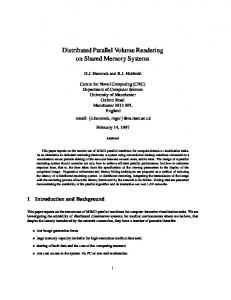
slice
2D grid
3D grid
Figure 1: Partitioning strategies for a voxel dataset.
was implemented by Schroeder and Salem [17] on a data-parallel computer (a Thinking Machine CM-2). A ray caster which works on multiprocessor workstations was proposed by Fruhauf [7]. The system is based on the transformation of the dataset from modeling space to viewing space. Rays are then casted by separate processors with ray direction always orthogonal to the viewing plane.
PARALLEL RAY TRACING OF REGULAR DATASETS In our project we concentrated on the parallel design of a RT algorithm to visualize voxel datasets on distributed-memory MIMD architectures. There are two aspects which warrant careful evaluation in order to give an efficient parallel implementation: parallelizing and data partitioning strategies.
Parallelizing and data partitioning strategies Badouel, Bouatouch and Priol [1] classified the parallelizing strategies for RT by focusing on the kind of data transmitted on the processor interconnection network. This classification can be assessed for volume RT as follows: • parallelism via image partition (also known as: parallelism without dataflow, or parallelism on pixels): a standard sequential RT implementation and the whole scene are replicated on each processing node. A partition of the image space identifies the subset(/s) of pixels that each node will independently synthesize. Implementations are straightforward and scalable, but the memory requirements are often prohibitive. • parallelism with ray dataflow: the scene data are partitioned and distributed to the processors. Each processor traces each ray in the local partition only. Each non-resolved ray is transmitted to “adjacent” processors for further tracing. The parallelization of RT sequential code is a complex task. • parallelism with object dataflow: a partition of the image is assigned to each processor, which locally traces and resolves each assigned ray. As in the previous strategy, scene data are partitioned among the processors, and an emulation of shared memory based on the transmission on request of data is therefore required. In volume RT the transmission of portions of high resolution datasets may involve large overhead and therefore this strategy is not at all effective. • parallelism on intersections: for each ray, a number of slave processors computes the ray–primitive intersections and returns them to a master, which sorts the intersections and computes shading. This strategy cannot be applied to volume RT, due to the simplicity of voxel tracing versus the higher cost of inter–node communications and the implicit ordering in voxel tracing.
Dataset Partition:
Image
Cluster 1 W1
....
Dataset allocation:
cluster 1
Cluster 2 Wn
W1
....
Wn cluster 2
.. .
Figure 2: A scalable parallel system based on a hybrid approach.
.. .
.. . cluster m
In volume RT the possible choices are therefore limited to image partition or ray dataflow. Partitioning a regular dataset is extremely simple because of the homogeneous and regular spatial distribution of the data. Some partitioning strategies are sketched in Figure 1: one–dimensional partitioning (slice partitioning) with the dataset divided into slices by using a set of parallel cutting planes; two–dimensional and three–dimensional partitioning, generated by means of 2D or 3D grids of orthogonal cutting planes or by the recursive subdivision in quadrant/octants. All of these strategies can be used to produce regular or adaptive partitions of the dataset. A ray tracer based on parallelism with ray dataflow entails subdividing the dataset, and therefore inter-node communications will be required for each ray that exits a partition allocated on one node and enters into an adjacent one. Each partitioning criterion implies different communications patterns between the RT processes. A bi-directional logical channel must connect each pair of nodes managing adjacent partitions, thus leading to a logical ring interconnection for the slice partitioning and 2D or 3D mesh interconnections for 2D or 3D grid partitioning, respectively. The topology of the underlying architecture generally influences the partitioning criteria. Due to the high number of messages interspersed with computations, an effective design of a parallel ray-dataflow RT algorithm must preserve communications locality by mapping the processes which hold adjacent partitions on neighbouring nodes in the hardware topology. A 3D grid partition strategy, for instance, is certainly not optimal if implemented on architectures with a lower dimensional topology (e.g. transputer–based architectures). Moreover, the more complex the interconnection is, the more complex will be the correct management of inter– node communications and deadlock prevention.
A hybrid parallelization approach to achieving high scalability The choice of a parallelism with ray dataflow to render volume datasets is justified by the following considerations: • the huge amount of memory needed to represent highresolution voxel datasets, even if the datasets have been previously classified and compressed, makes partitioning and distributing the data a must. This is due to the limitation of the local RAM space and the lack of virtual memory management common to most multicomputers. • regular dataset subdivision into distinct partitions is simple and does not involve all the problems inherent in boundary or CSG scene partitions (e.g. elementary primitive spanning more than one partition). • visual realism is not as important as in high-quality rendering. Users of volume rendering applications are generally more concerned with knowledge of the represented phenomena than with excessive realism. This
worker1 worker2 worker3 worker4 slice 1
slice 3 slice 2 slice 4
Figure 3: Allocation of the voxel dataset on the processing nodes (in the example, a configuration with four nodes per cluster is shown).
means fewer number of rays generated in the image synthesis process and fewer ray transmissions on the communications network, and thus lower communications overhead and simpler load balancing. Adopting a slice partitioning strategy is justified in terms of ease of implementation, management and load balancing, as the following points show: • partitioning the dataset into slices and transmitting them to the processing nodes is straightforward; • the communications pattern between nodes is very simple; • the simple partition criterion also allows extremely simple load balancing, based on dataset partition modification. By shifting the cutting planes, the node load can be easily optimized without altering the adjacency relation between nodes. Due to communications overhead, the scalability of a slice-based RT is low. However, the exploitation of high parallelism (e.g. 102 or more processors) is prevented even if different partitioning strategies (e.g. 2D or 3D grids) are applied. The relative simplicity of tracing regular datasets makes the trade-off between computation and interprocessor communication extremely costly, as the mean length of the ray traced by each node is reduced to a few tenths of voxels. Whichever partition criterion is chosen, effective scalability of the ray dataflow solution is unlikely to be achieved by simply increasing the number of partitions, with the resolution of the data unchanged. In other words, only when the dataset resolution increases can a proportional increase in the exploited parallelism be gained through finer partitioning of the dataset space. Following the above guidelines, a highly parallel volume raytracing system can only be designed by applying a ray dataflow approach within an image partition approach (Figure 2). The computing nodes can be organized into a set of clusters, each of them composed of the same number of nodes. The image space is partitioned and a subset of pixels is assigned to each cluster, which will compute pixel values independently. Each cluster is composed of a set of co-operating nodes, working under a ray dataflow approach. The dataset is replicated on each cluster, and is partitioned among the local memory of the cluster’s nodes. In order to optimize global efficiency the number of nodes per clusters is chosen as a function of dataset resolution.
VOLUME RT ON A HYPERCUBE ARCHITECTURE The proposed hybrid solution was implemented on a highly parallel hypercube multicomputer, an nCUBE 2 system, model 6410, populated with 128 processing nodes each with 4 Mbytes of local memory. Running at a clock rate of 20 MHz, the nCUBE node processor is rated at 7.5 MIPS and 3.3 MFLOPS, single precision, or 2.4 MFLOPS, double precision. The datasets are stored on the nCUBE file system in four one-Gbytes disks which are managed by the same number of I/O processors. Due to the lack of a graphics board, the images computed on the hypercube are visualized under the X11 environment of the host workstation.
The software architecture The proposed parallel algorithm derives from the volume RT algorithm described in [13]. The parallel algorithm was designed by using a hybrid image partition – ray dataflow approach leading to a set of processes which communicate following a mesh pattern. To embed the process graph into the hypercube topology (Figure 3), the P = 2k nodes of the parallel system were logically divided into m = 2i clusters, composed of cd = 2k−i nodes interconnected in a ring (cd=cluster dimension). Such an embedding can be built so that the neighbourhood relations are preserved [15]. The image synthesis process is divided among clusters with a without dataflow approach. The strategy chosen to partition the image between clusters is extremely simple: the image is divided into rows of pixels; row ri , with 1 ≤ i ≤ N and N ∗ N the image resolution, is assigned for computation to the (i DIV m)th cluster. The resulting load is balanced because the time for the synthesis of rows which are adjacent or close in the image is nearly equal, if the hypothesis of N >> m holds. The same code runs on each processing node, known as a worker. Each worker computes its cluster number and position inside the cluster with simple transformations of the hypercube nodeid (the identification code assigned to each node) [15]. The tracing process is parallelized at the cluster level with a ray dataflow approach. The dataset is partitioned into slices, and each slice sj of the volume data is replicated on the local memory of the node wj on all the clusters (Figure 3). The position inside a cluster of a node univocally identifies the dataset slice assigned to it. Each node can therefore asynchronously load the data subset contained in the assigned space partition from secondary storage. Volume ray tracing consists of a simple incremental scan conversion of the ray in order to identify all of the voxels which are crossed by the ray. For each sampling point on the ray, the algorithm reads from the voxel dataset or interpolates the sampling point value on the cell dataset. If the algorithm detects a threshold crossing, the ray has traversed an iso–surface and shading computation is applied. Depending on the transparency coefficient associated with the field value, ray tracing is either stopped or continues to search for other threshold voxels. If the ray exits the space partition assigned to the worker without hitting any threshold voxel, two different outcomes can occur. If the ray enters the partition assigned to an adjacent worker, the current worker stops tracing and transmits the ray description to the adjacent one. The adjacent worker
will continue tracing that ray in its dataset partition. Otherwise, if the ray exits from the global bounding volume of the dataset, tracing stops and the color contribution of the ray is computed. Each worker manages the generation of all the primary rays assigned to its cluster. It intersects each ray with the bounding volume (bvol) of the dataset. If the first ray-bvol intersection is located on the frontier of the local partition, then the worker starts tracing it, otherwise the primary ray is rejected. The drawback of this distributed primary ray generation strategy is that for each pixel row assigned to the cluster, the associated primary rays are generated and checked on all the worker nodes in the cluster. Alternatively, using a centralized strategy, primary rays can be generated and tested for intersection on a single node (e.g. on the host) and each ray transmitted to the worker whose space partition is traversed first by the ray. The centralized strategy leaves the nodes active on effective tracing only. On the other hand, the distributed policy involves a significant reduction in communications overhead. Since primary rays are generated on request, workers do not need to read them from the communications buffer of the node. The advantage is lower size and faster management of the communications buffer, because the nCUBE system primitives testing for the presence of, or getting messages from, the communications buffer have a complexity proportional to the buffer size and the number of messages currently pending. A distributed strategy enables generating primary rays on each node when no ray tracing requests from adjacent nodes are pending in the communication buffer. This solution positively affects both load balancing and deadlock prevention. The recursive RT process can be completed by a single node wi , or distributed on a number of co-operating nodes. If it is possible to trace the whole ray tree in the wi space, the color contributions of these rays are composed to give the resulting pixel value. Otherwise, each ray rk in the tracing tree, which exits the space partition of wi and enters those of an adjacent node wj , has to be transmitted to wj for further tracing. At this point, wi has to wait for a ray descriptor, relative to rk and containing its computed color contribution, to return from wj . In order to prevent active waiting, wi saves the current state of the computation on a primary ray descriptor and starts tracing another ray. The worker process will terminate the computation of the pixel color associated with that previous primary ray when it receives a ray descriptor containing the resolved rk and its color contribution from a node of the cluster. Shadow rays are managed the same way as transparency rays: if they cannot be completely traced in the current partition, they are transmitted to the adjacent node and the worker saves the current tracing status in order to restore it as soon as the resolved ray descriptor is received. The worker manages a list of partially processed primary ray descriptors. Each of these contains: the primary ray direction, its starting point and, if necessary, the resolved intersection p1 , the generated secondary rays and their respective intersections, etc. All this status information results in a further list of descriptors, one for each non-resolved secondary ray. The efficiency of the system might be increased by the use of 3D shadow buffers, as proposed in [4]. The use of this technique bring about a reduction of the secondary rays to be traced and consequently of the internode communica-
tions. Nevertheless, the increased memory requirements of this technique (to storing the l 3D grids of shadowing info, with l the light source number) make it mandatory to partition the data and adopt of a ray dataflow strategy. Each primary ray descriptor is created dynamically as soon as a worker starts to trace a primary ray. The list is then held in the local memory of the worker which finds the first intersection of the primary ray with a threshold voxel. The primary ray descriptor is therefore created by the worker wi , which starts to trace the ray, and then transmitted to the adjacent worker if wi does not find an intersection in its partition. Once all rays associated with a primary ray are traced, the pixel color is computed on the basis of the threshold voxels intersected, the characteristics of the associated iso– surfaces and the normal vector approximated at the intersection points pi . The normal vector at point pi is approximated by using an object-space gradient method [19] with the gradient computed from the value of a set of voxels at a distance of p steps from pi in voxel–based datasets, or as the field gradient, in cell–based datasets. If pi is on the boundary of the partition, then some of the required neighbouring voxels/cell nodes might be in the adjacent node’s local memory. In order to avoid the necessary management of these requests for external voxel values, and the associated overhead, we allocate to each worker a dataset slice which is larger than the associated partition (i.e. g voxel planes larger on both sides where g is the maximum width of the 3D interval needed for gradient computation). The current implementation can be easily extended to apply a compositive approach instead of a surface-searching one. System performance should not be significantly altered when a compositive shading model is used. Deadlock prevention and termination algorithms A peculiar characteristic of parallel raytracers with ray dataflow are deadlock occurrences and the fact that each tracer process cannot locally determine its termination. Deadlocks may occur between two or more workers in a cluster in the case they form a cyclic dependency when waiting for messages, and no message can advance toward its destination because the nodes’ communications buffers are full. A slice partition strategy may cause cyclic dependency between workers even if the flow of all the rays follows the direction of the view (i.e. the user has positioned all light sources so that shadow rays are traced in the same direction as the view direction). In fact, the resolved secondary rays with their color contribution return to the workers in which the first intersection of the primary ray was found. To avoid deadlock it is therefore necessary to prevent the node communications buffers from being filled up. In our solution the node communications buffer cannot be exhausted because we have designed a monitoring mechanism based on acknowledgement of the receipt of messages from the destination workers. Each worker manages a set of counters ni to trace the messages sent to a destination but not yet received by the receiver. The counter ni increases when a message is sent to worker wi and decreases when the node receives the acknowledgement message ack from wi . Each worker can send a new message to wi only if ni is lower than a value imax which is determined as a function of the size of the communication buffer, the size of messages and the
...
W2
W1 tt1
tt2
Wn ttn
Cluster j TTj
Host
Primary rays' flow
Figure 4: Termination management via termination token transmission (in the example, the view point is on the left of the dataset, hence the primary ray propagation is in the direction shown).
number of workers in a cluster. Furthermore, the worker can begin to trace a new (primary or secondary) ray only if the relation ni + rimax < imax holds, where rimax is the maximum number of potential communications to the worker wi required to trace that ray. The value of rimax can be simply computed as a function of the type of ray and the number of light sources in the scene. If a worker cannot trace a new ray, it waits to receive ack or ray messages from the other nodes. In order to increase efficiency, priority is given, in this order: to ack messages, resolved ray descriptors and new rays coming from adjacent workers. Only when the buffer of incoming messages is empty does a worker generate a new primary ray and begin to trace it. The particular organization of the proposed solution makes the termination algorithm extremely simple. Termination control is managed by using m termination tokens, one for each cluster (Figure 4). On each cluster, the termination token is generated by the node w whose dataset partition is nearest to the view point (i.e., node w is w1 or wn ). The tokens are transmitted between cluster nodes following the direction of propagation of primary rays. Each node wj receives the token and transmit it to the adjacent node as soon as all the pixels associated with the primary rays generated by wj are rendered. The node which is furthest from the view point transmits the token to the host upon termination of local pixels rendering. The host terminates the run as soon as it receives the mth token, with m the number of clusters. Load balancing Dynamic load balancing methods generally involve a high degree of message interchange in order to synchronize and move data between nodes. In some cases the strategies are complex and require partition modification and dynamic reallocation of the data. Furthermore, it is difficult to manage the frequency of load redistribution and the behaviour of the system under multiple partition redistribution. The technique we implemented is a static technique similar to that proposed by Priol, et al. [14]. It is based on redistribution of the data depending on the estimated workload of each processor. As described above the initial data partitioning is uniform. To choose a more effective distribution of the dataset the host asks one cluster to trace a subset of primary rays, regularly distributed on the image plane (for example a regular grid of 16 ∗ 16 or 32 ∗ 32 rays).
On the basis of the total time ti spent by the worker wi to trace these test rays, the host defines a new subdivision of the dataset, with size[i] of the new partition computed as: size[i] = size[i] + (tmean − ti )/tsingle−plane where tmean is the meanP processing time on the worker nodes, and tsingle−plane = (ti )/n, with n the resolution of the dataset on the X axis. In order to achieve the new distribution, each worker node transfers data to (and/or acquires it from) its neighbour nodes; this data transmission process is performed in parallel by the workers of each cluster. The technique is effective, because the redistribution time is much lower than the image synthesis time. The substantial speedup obtained is reported in Table 3.
Scalability In designing the system one of the main goals was the efficient exploitation of high parallelism. To achieve optimum system scalability, the flexibility of the hybrid parallelism has to be carefully exploited. In fact, depending on the specific characteristics of the datasets to be visualized and on the requested visualization parameters (i.e. lights, projection and view settings), a particular parallelism strategy and degree may result in lower image synthesis time. So, for each visualization request, the user selects the dimension p of the hypercube to be used and the number of clusters in which the cube has to be configured. For example, the user can choose to synthesize the image following a pure image partition approach by selecting a unitary dimension for the clusters; on the other hand , a pure ray dataflow approach can be applied by configuring the system as a single cluster of 2p nodes. The flexibility of the system allows for the selection of the most suitable parallelization scheme, which results in higher efficiency and interactive time in image synthesis.
The host interface The host workstation has management and I/O functions only. It manages two main activities: (a) input file scanning and hypercube management, (b) result (images) collection and timing. (a) Input file scanning: the host reads in the input file specified by the user, which contains the selection of one or more datasets plus the related visualization specifications. For each selected dataset the user specifies one or more set of visualization parameters (i.e. projection and view settings, threshold surface coefficients, etc.) and the dimensions and configuration (i.e. the number of clusters) of the hypercube to be used for the synthesis of the image. For each dataset to be visualized, the host allocates the requested hypercube, loads each node with the executable worker code and broadcasts the visualization parameters specified by the user to the worker nodes. (b) Images and timing collection: the workers trace the image and send the evaluated pixels to the host node. To minimize overhead, the workers accumulate pixel values and transmit pixel sets to the host with a single message. At the end of the image synthesis process, each worker sends monitoring and statistical data back to the host.
RESULTS Results showing the system’s effective exploitation of parallelism are presented in Table 1. The table contains the times relative to the image synthesis at a resolution of 350x250 from a 97x97x116 dataset which represents the electron density map of an enzyme (SOD, Super Oxide Dismutase). The dataset has been chosen for its wide–spread use, in order to facilitate comparison with other experiences. The test images, reproduced in Figure 5, are generated with a view direction which forms a 45 degree angle with the Z and X axes and orthogonal to the Y axis. The projection of the dataset on the image plane covers an area of 301x194 pixels, and the distance between ray samples is 1/2 of the cell edge. Both times and efficiencies are in Table 1. The analysis of the efficiency is more suitable for evaluating system performance because the actual times suffer from both the limited speed of the nCUBE node processor with respect to the more powerful RISC workstation processors and the lack of optimization of the sequential raytracer used. No acceleration techniques, such as Levoy’s octree [11] or that proposed in [13], are used in the current implementation; the system is amenable to acceleration techniques which should result in performance enhancements similar to those reported for sequential raytracers. Table 2 reports the times and the efficiency measured on the same dataset of Table 1 using a different configuration of the hypercube nodes: the hypercube dimensions are fixed, and the number of nodes in each cluster decreases from 16 to 1. Table 3 reports the times and the efficiency measured on the same dataset, with and without the use of the load balancing option. Table 4 presents the profile analysis of a run on a single cluster composed of 16 nodes. The dataset and image characteristics are the same as the previous tables, and therefore the use of a 16 node cluster involves the not negligible communication overhead shown. Only the percentage times of the more time consuming procedures are reported. Ntest is the system function used to test the presence of messages in the communication buffers; nread and nwrite are the communication primitives, the classical CSP send and receive; Trace implements ray sampling; Interpolate interpolates the cell–based dataset to compute sample point values; V oxel Sample manages threshold searching and shading. The synthesis of 1024x768 images of the SOD dataset, with the distance between ray samples equal to 1/5 of the cell edge (the projected dataset containment box is 748x482 pixels wide), requires 1’20” with efficiency 0.82 using all 128 nodes of the hypercube.
CONCLUSIONS A proposal for a distributed-memory parallel system to render volumetric datasets has been presented. The methodology and parallelization strategy followed in the system design have been described and justified. Using a ray tracing approach, the system renders volumetric datasets which are coded in a voxel–based or cell–based representation scheme. It adopts a hybrid image partition – with ray dataflow approach based on a slice partitioning of the dataset. Simple and efficient procedures for minimizing communications
overhead, for termination detection and for static load balancing have been implemented and evaluated. The reported results show that the proposed hybrid parallelization strategy fulfils the initial goal: the visualization of high resolution volume dataset on MIMD distributed memory architectures which are characterized by a low I/O bandwidth and a reduced amount of local memory. More than the actual run times, which suffer from shortcomings of the base algorithm used, the efficiency obtained for such a highly communicating algorithm (0.74 on 128 nodes) is higher than those reported elsewhere and validates the correctness of the design choices. Acknowledgements This work was partially funded by the Progetto Finalizzato “Sistemi Informatici e Calcolo Parallelo” of the Consiglio Nazionale delle Ricerche. The electron density map dataset was provided by Duncan Mc Ree, Scripps Clinic, La Jolla (CA). We also thank the University of North Carolina at Chapel Hill for having collected and made available the above and other datasets. The authors also thank Paolo Bussetti and Luca Misericordia for their valuable contribution to the system implementation.
REFERENCES [1] Badouel, D., Bouatouch, K., and Priol, T. Ray tracing on distributed memory parallel computers: strategies for distributing computations and data. In Parallel Algorithms and Architectures for 3D Image Generation - ACM SIGGRAPH ’90 Course Note no.28 (July 1990), pp. 185–198. [2] Challinger, J. Object Oriented Rendering of Volumetric and Geometric Primitives. PhD thesis, University of California, Santa Cruz, CA, 1990. [3] Challinger, J. Parallel volume rendering on a sharedmemory multiprocessor. Tech. Rep. CRL 91-23, University of California, Santa Cruz, CA, July 1991. [4] Ebert, D., and Parent, R. Rendering and animation of gaseous phenomena by combining fast volume and scanline a-buffer techniques. A.C.M. Computer Graphics 24, 4 (August 1990), 357–366. [5] Foley, J., van Dam, A., Feiner, S., and Hugues, J. Computer Graphics: Principles and Practice - Second Edition. Addison Wesley, 1990. [6] Frenkel, K. Volume rendering. Comm. ACM 32, 4 (April 1989), 426–435. [7] Fruhauf, T. Volume rendering on a multiprocessor architecture with shared memory: A concurrent volume rendering algorithm. In 3rd EuroGraphics Workshop on Scientific Visualization (Pisa, April 1992). [8] Glassner, A. An Introduction to Ray Tracing. Academic Press, 1989. [9] Kaufman, A., Bakalash, R., Cohen, D., and Yagel, R. A survey of architectures for volume rendering. IEEE Engineering in Medicin and Biology (Dec. 1990), 18–23. [10] Levoy, M. A hybrid raytracer for rendering polygon and volume data. IEEE C. G.& A. 10, 2 (March 1990), 33–40.
[11] Levoy, M. Volume rendering by adaptive refinements. ACM Trans. on Graphics 9, 3 (July 1990). [12] Lorensen, W., and Cline, H. Marching cubes: a high resolution 3d surface construction algorithm. ACM Computer Graphics 21, 4 (1987), 163–170. [13] Montani, C., and Scopigno, R. Rendering volumetric data using the sticks representation scheme. ACM Computer Graphics 24, 5 (November 1990), 87–94. [14] Priol, T., and Bouatouch, K. Static load balancing for a parallel ray tracing on a mimd hypercube. The Visual Computer 5, 1/2 (March 1989), 109–119. [15] Ranka, S., and Sahni, S. Hypercube Algorithms. Springer–Verlag, New York, 1990. [16] Reynolds, R. A., Gordon, D., and Chen, L. A dynamic screen technique for shaded graphics display of slice-represented objects. Computer Graphics and Image Processing, 38 (1987), 275–298. [17] Schroder, P., and Salem, J. Fast rotation of volume data on data parallel architectures. In Proceedings of IEEE Visualization ’91 (October 1991). [18] Stytz, M., Frieder, G., and Frieder, O. Threedimensional medical imaging: Algorithms and computer systems. ACM Computing Survey 23, 4 (December 1991), 421–499. [19] Tiede, U., Hoene, K., Bomans, M., Pommert, A., M.Riemer, and Wiebecke, G. Investigation of medical 3d-rendering algorithms. IEEE C. G.& A. 10, 2 (March 1990), 41–53. [20] Upson, C., and Keeler, M. V-buffer: Visible volume rendering. ACM Computer Graphics 22, 4 (August 1988), 59–64. [21] Westover, L. Footprint evaluation for volume rendering. ACM Computer Graphics 24, 4 (July 1990), 367–376. [22] Wilhelms, J. Decisions in volume rendering. In State of the Art in Volume Visualization - ACM SIGGRAPH ’91 Course Note No.8 (July 1991), pp. 1–11. [23] Wilhelms, J., and Gelder, A. V. A coherent projection approach for direct volume rendering. ACM Computer Graphics 25, 5 (July 1991), 275–284. [24] Yazdy, F., Tyrrel, J., and Riley, M. Carvupp: Computer assisted radiological visualization using parallel processing. In NATO ASI Series - 3D Imaging in Medicine (1990), K. H. H. et al., Ed., vol. F60, Springer-Verlag, pp. 363–375.
Timings 1node 2nodes 4nodes 8nodes 16nodes 32nodes 64nodes 128nodes
time 485.24 260.35 130.19 65.82 32.96 17.26 8.90 5.14
speedup 1 1.86 3.73 7.37 14.72 28.11 54.52 94.41
ef f iciency 1 0.93 0.93 0.93 0.92 0.88 0.85 0.74
Table 1: Times (in seconds), speedup and efficiency of the visualization of the SOD dataset with increasing number of nodes.
Cluster size 64nodes, times ef f iciency 128nodes, times ef f iciency
16 24.16 0.31 12.32 0.31
8 17.16 0.44 8.77 0.43
4 11.93 0.64 6.70 0.57
2 10.10 0.75 5.14 0.74
1 8.90 0.85 6.42 0.59
Table 2: Times (in seconds) and efficiency measured on the SOD dataset with decreasing cluster size.
Cluster size 64nodes standard times 64nodes balanced times 128nodes standard times 128nodes balanced times
16
8
4
2
24.16
17.16
11.93
10.10
15.20
12.26
10.26
9.27
12.32
8.77
6.70
5.14
7.94
6.56
6.04
4.75
Table 3: Comparison between the times (in seconds), with or without the adopted load balancing technique, for the visualization of the SOD dataset with decreasing clusters size.
Profiling ntest Interpolate T race V oxel Sample nread nwrite
M ean 32.82 31.48 9.39 8.46 1.36 1.38
M in 0.77 20.96 6.60 5.60 1.02 0.83
M ax 46.82 55.55 15.55 14.77 1.76 2.08
Table 4: Profile analysis on a single 16–node cluster.