Implementation and Evaluation of Algorithmic Skeletons: Parallelisation of Computer Algebra Algorithms Dissertation zur Erlangung des Doktorgrades der Naturwissenscha en (Dr. rer. nat.)
dem
F
P
M
-U vorgelegt von
Oleg Lobachev aus Gießen
Marburg/Lahn,
I M
Implementation and Evaluation of Algorithmic Skeletons: Parallelisation of Computer Algebra Algorithms Oleg Lobachev th November
Contents from our own publications [Lobachev and Loogen, , Berthold et al., b, Lobachev and Loogen, a] have been reproduced with a kind permission of Springer-Verlag Berlin / Heidelberg, Germany. Contents from our own publication [Lobachev and Loogen, c] has been reproduced with a kind permission of ACM New York, NY, USA. Figure . is a redrawn version of a part of Figure . from [von zur Gathen and Gerhard, ].
Vom Fachbereich Mathematik und Informatik der Philipps-Universität Marburg als Dissertation am .. angenommen. Tag der mündlichen Prüfung: ... Erstgutachterin: Prof. Dr. Rita Loogen Zweitgutachterin: Prof. Dr. Yolanda Ortega Mallén
Abstract is thesis presents design and implementation approaches for the parallel algorithms of computer algebra. We use algorithmic skeletons and also further approaches, like data parallel arithmetic and actors. We have implemented skeletons for divide and conquer algorithms and some special parallel loops, that we call ‘repeated computation with a possibility of premature termination’. We introduce in this thesis a rational data parallel arithmetic. We focus on parallel symbolic computation algorithms, for these algorithms our arithmetic provides a generic parallelisation approach. e implementation is carried out in Eden, a parallel functional programming language based on Haskell. is choice enables us to encode both the skeletons and the programs in the same language. Moreover, it allows us to refrain from using two different languages—one for the implementation and one for the interface—for our implementation of computer algebra algorithms. Further, this thesis presents methods for evaluation and estimation of parallel execution times. We partition the parallel execution time into two components. One of them accounts for the quality of the parallelisation, we call it the ‘parallel penalty’. e other is the sequential execution time. For the estimation, we predict both components separately, using statistical methods. is enables very confident estimations, although using drastically less measurement points than other methods. We have applied both our evaluation and estimation approaches to the parallel programs presented in this thesis. We haven also used existing estimation methods. We developed divide and conquer skeletons for the implementation of fast parallel multiplication. We have implemented the Karatsuba algorithm, Strassen’s matrix multiplication algorithm and the fast Fourier transform. e latter was used to implement polynomial convolution that leads to a further fast multiplication algorithm. Specially for our implementation of Strassen algorithm we have designed and implemented a divide and conquer skeleton basing on actors. We have implemented the parallel fast Fourier transform, and not only did we use new divide and conquer skeletons, but also developed a map-and-transpose skeleton. It enables good parallelisation of the Fourier transform. e parallelisation of Karatsuba multiplication shows a very good performance. We have analysed the parallel penalty of our programs and compared it to the serial fraction—an approach, known from literature. We also performed execution time estimations of our divide and conquer programs. is thesis presents a parallel map+reduce skeleton scheme. It allows us to combine the usual parallel map skeletons, like parMap, farm, workpool, with a premature termination property. We use this to implement the so-called ‘parallel repeated computation’, a special form of a speculative parallel loop. We have implemented two probabilistic primality tests: the Rabin–Miller test and the Jacobi sum test. We parallelised both with our approach. We analysed the task distribution and stated the fitting configurations of the Jacobi sum test. We have shown formally that the Jacobi sum test can be implemented in parallel. Subsequently, we parallelised it, analysed the load balancing issues, and produced an optimisation. e latter enabled a good implementation, as verified using the parallel penalty. We have also estimated the performance of the tests for further input sizes and numbers of processing elements. Parallelisation of the Jacobi sum test and our generic parallelisation scheme for the repeated computation is our original contribution. e data parallel arithmetic was defined not only for integers, which is already known, but also for rationals. We handled the common factors of the numerator or denominator of the fraction with the modulus in a novel manner. is is required to obtain a true multiple-residue arithmetic, a novel result of our research. Using these mathematical advances, we have parallelised the determinant computation using the Gauß elimination. As always, we have performed task distribution analysis and estimation of the parallel execution time of our implementation. A similar computation in Maple emphasised the potential of our approach. Data parallel arithmetic enables parallelisation of entire classes of computer algebra algorithms. Summarising, this thesis presents and thoroughly evaluates new and existing design decisions for high-level parallelisations of computer algebra algorithms.
Abstract (Deutsch) Die vorliegende Arbeit beschreibt den Entwurf und die Implementierung paralleler Computeralgebraalgorithmen mithilfe von algorithmischen Skeletten und weiteren Ansätzen, wie datenparallele Arithmetik und Actors. Wir implementieren algorithmische Skelette für Divide and Conquer und spezielle, spekulative parallele Schleifen. Ähnlich zu den Skeletten ist die rationale datenparallele Arithmetik ebenfalls ein Parallelisierungschema, allerdings ist dieses speziell für Algorithmen der Computeralgebra ausgelegt. Die Parallelisierung wird in der parallelen funktionalen Sprache Eden vorgenommen. Eden ist eine Erweiterung von Haskell. Mit Eden ist es möglich, sowohl die Skelette als auch die Programme in einer Sprache zu definieren. Ein ähnlicher Ansatz erlaubt uns, die „innere“ und die „äußere“ Sprache einer Computeralgebra-Implementierung zu vereinigen. Desweiteren schlägt diese Arbeit eine Methode zur Auswertung und Abschätzung der parallelen Laufzeiten vor. Im Gegensatz zu den gängigen Ansätzen werden statistische Verfahren verwendet. Dadurch können wir sehr überzeugende Vorhersagen liefern. Im Vergleich zu den anderen Verfahren verwenden unsere Methoden deutlich weniger Datenpunkte. Eine von uns eingeführte Komponente der parallelen Laufzeit erlaubt eine strikte Kontrolle der Güte der Parallelität. Wir führen sowohl die Qualitätsmerkmale als auch die Abschätzung der parallelen Laufzeit für die in der Arbeit vorgestellte Implementierungen aus. Mit den Divide and Conquer Skeletten werden die Algorithmen für schnelle Multiplikation, nämlich Karatsuba Algorithmus und Strassen Matrixmultiplikation sowie die schnelle Fouriertransformation, entwickelt. Letzteres wird auch mit einem map-and-transpose Skelett umgesetzt. Damit haben wir eine gute Parallelisierungmerkmale beobachtet. Wir verwenden die schnelle Fouriertransformation, um eine schnelle Faltung von Polynomen umzusetzen, was zu einem weiteren Algorithmus zur schnellen Multiplikation führt. Der parallele Algorithmus von Karatsuba zeigt sehr gute Parallelisierungmerkmale. Für den Algorithmus von Strassen implementieren wir ein Actors-basiertes Divide and Conquer Skelett. Wir analysieren die Messungen ausführlich, um die Güte der Parallelisierung sicherzustellen. Wir stellen ein map+reduce Schema vor. Es erlaubt, gängige parallele Skelette wie parMap, farm, workpool mit einer Abbruchsklausel zu versehen. Wir setzen mit diesem Skelettschema die Algorithmen zu probabilistischen Primzahlprüfung um. Wir implementieren den Rabin–Miller-Test und den Jacobi-Summen-Test. Bei dem ersten optimieren wir die Aufgaben- und Prozessorenanzahl. Bei dem Jacobi-Summen-Test beweisen wir zuerst, dass es überhaupt möglich ist, unseren Ansatz zu verwenden. Danach wird die Implementierung erzeugt und parallelisiert. Dabei nehmen wir eine Optimierung der Aufgabenreihenfolge vor, was die Speedup Werte deutlich verbessert. Ebenfalls werden auch hier die beiden Implementierungen ausführlich analysiert. Die Laufzeiten werden für weitere Problemgrößen und Prozessorenzahlen abgeschätzt. Die datenparallele Arithmetik wurde nicht nur für ganze Zahlen, sondern auch für Brüche umgesetzt. Wir stellen eine neuartige Lösung vor, die die gemeinsamen Faktoren des Zähler oder Nenner des Bruches mit der Zahl eliminiert, modulo der man rechnet. Das ist notwendig um eine hinreichende Skalierung der multimodularen Arithmetik zu ermöglichen. Unter Verwendung dieser Erkenntnisse haben wir die Determinantenberechnung mittels Gauß Elimination parallelisiert. Eine vergleichbare Berechnung in Maple zeigte die großen Vorteile unseres Ansatzes. Die vorliegende Dissertation präsentiert Implementierung und gründliche Auswertung von highlevel Parallelisierungen verschiedener Computeralgebraalgorithmen.
To my mother
ACKNOWLED GEMENTS
of all I would like to thank my thesis adviser Prof. Dr. Rita Loogen for the invaluable collaboration and support. Her supervision and encouragement made this work possible in the first place. I am very grateful to Prof. Dr. Yolanda Ortega-Mallén for her deep and helpful comments. Further, I would like to thank my colleagues Dr. Jost Berthold, Mischa Dieterle, Prof. Dr. Michael Guthe and omas Horstmeyer for collaboration and discussions. Dominik Krappel, Kent Kwee, Bernhard Pickenbrock, Florian Pfeiffer and Steffen Vaupel supported the implementation of the codebase, which is used in this thesis. I was also lucky to have fruitful discussions with Paolo Giarrusso, Egbert Fohry, Kathi Haselhorst and Tillmann Rendel. I want to specially thank Tillmann for the discussion on monoids and many other very interesting conversations. I benefited from the collaboration with my colleagues in Scotland: I thank Prof. Dr. Phil Trinder and Dr. Abyd Al Zain for the possibility to use the Beowulf cluster of the Heriot-Watt University. Further, I thank Dr. Alexander Konovalov (University of St. Andrews) for his support. Dr. Siarhei Khirevich and Anton Daneyko from the Faculty of Chemistry at Philipps-Universität Marburg kindly provided me their run time measurements on a supercomputer. ese helped me a lot. A loud ‘thank you’ goes to Mark Schäfer and all my former colleagues at Identass GmbH & Co. KG for the possibility to work together in the first phase of this project. e material for this work emerged under the support of Deutsche Forschungsgemeinscha under the grant number LO -/ and Hessian Ministry for Science and the Arts’ HMWK LOEWE KMU programme. I am very grateful to my family for all support and patience I enjoy. I deeply appreciate all and every kind of assistance, my parents give to me.
F
Oleg Lobachev
i
CONTENTS
Acknowledgements
i
Contents
iii
1
Introduction 1.1 Parallel Programming . . . . . . . . . . . . . . . . . . . . . . . . . . . . . . . . . . . . . . 1.2 Goals of is Work . . . . . . . . . . . . . . . . . . . . . . . . . . . . . . . . . . . . . . . 1.3 Structure of e esis . . . . . . . . . . . . . . . . . . . . . . . . . . . . . . . . . . . . .
2
Programming Languages And Symbolic Computation 2.1 Symbolic Computation . . . . . . . . . . . . . . . . 2.2 Language Unity . . . . . . . . . . . . . . . . . . . . 2.3 Dependent Typing . . . . . . . . . . . . . . . . . . . 2.4 An Example: Laziness . . . . . . . . . . . . . . . . . 2.5 Conclusions and Outlook . . . . . . . . . . . . . . .
. . . . .
. . . . .
. . . . .
. . . . .
. . . . .
. . . . .
. . . . .
. . . . .
. . . . .
. . . . .
. . . . .
. . . . .
. . . . .
. . . . .
. . . . .
. . . . .
. . . . .
. . . . .
. . . . .
. . . . .
. . . . .
7 8 9 11 12 14
Parallel Programming With Eden 3.1 Eden as Haskell Extension . 3.2 Skeletons Survey . . . . . . . 3.3 Eden Tracing . . . . . . . . . 3.4 Measurement Methodology 3.5 Conclusions . . . . . . . . .
. . . . .
. . . . .
. . . . .
. . . . .
. . . . .
. . . . .
. . . . .
. . . . .
. . . . .
. . . . .
. . . . .
. . . . .
. . . . .
. . . . .
. . . . .
. . . . .
. . . . .
. . . . .
. . . . .
. . . . .
. . . . .
15 16 22 35 36 37
3
4
5
6
. . . . .
. . . . .
. . . . .
. . . . .
. . . . .
. . . . .
. . . . .
. . . . .
. . . . .
. . . . .
. . . . .
. . . . .
. . . . .
1 2 4 5
Estimating Parallel Performance 4.1 Related Work for Parallel Performance . . . . . 4.2 Our View on Parallel Computation . . . . . . . 4.3 Estimation . . . . . . . . . . . . . . . . . . . . . 4.4 Example I: Hamming Numbers . . . . . . . . . 4.5 Example II: Lattice-Boltzmann Method . . . . 4.6 Comparing Serial Fraction and Parallel Penalty 4.7 Related Work on Performance Estimation . . . 4.8 Conclusions . . . . . . . . . . . . . . . . . . . .
. . . . . . . .
. . . . . . . .
. . . . . . . .
. . . . . . . .
. . . . . . . .
. . . . . . . .
. . . . . . . .
. . . . . . . .
. . . . . . . .
. . . . . . . .
. . . . . . . .
. . . . . . . .
. . . . . . . .
. . . . . . . .
. . . . . . . .
. . . . . . . .
. . . . . . . .
. . . . . . . .
. . . . . . . .
. . . . . . . .
. . . . . . . .
. . . . . . . .
. . . . . . . .
39 40 41 42 43 44 48 50 50
Primality Testing — Repeated Computation 5.1 Repeated Computation Skeletons . . . . 5.2 Map+Reduce . . . . . . . . . . . . . . . . 5.3 Case Studies . . . . . . . . . . . . . . . . 5.4 Rabin–Miller Test . . . . . . . . . . . . . 5.5 Jacobi Sum Test . . . . . . . . . . . . . . 5.6 Conclusions . . . . . . . . . . . . . . . .
. . . . . .
. . . . . .
. . . . . .
. . . . . .
. . . . . .
. . . . . .
. . . . . .
. . . . . .
. . . . . .
. . . . . .
. . . . . .
. . . . . .
. . . . . .
. . . . . .
. . . . . .
. . . . . .
. . . . . .
. . . . . .
. . . . . .
. . . . . .
. . . . . .
. . . . . .
. . . . . .
. . . . . .
. . . . . .
. . . . . .
. . . . . .
51 51 55 61 62 67 89
Fast Multiplication — Divide and Conquer 6.1 History . . . . . . . . . . . . . . . . . . 6.2 Divide and Conquer Skeletons . . . . . 6.3 Univariate Polynomials . . . . . . . . . 6.4 Fast Fourier Transform . . . . . . . . . 6.5 Matrices . . . . . . . . . . . . . . . . . .
. . . . .
. . . . .
. . . . .
. . . . .
. . . . .
. . . . .
. . . . .
. . . . .
. . . . .
. . . . .
. . . . .
. . . . .
. . . . .
. . . . .
. . . . .
. . . . .
. . . . .
. . . . .
. . . . .
. . . . .
. . . . .
. . . . .
. . . . .
. . . . .
. . . . .
. . . . .
91 . 92 . 94 . 98 . 107 . 127
. . . . .
iii
iv
Contents 6.6 6.7
7
8
Divide and Conquer with Actors . . . . . . . . . . . . . . . . . . . . . . . . . . . . . . . 135 Conclusions . . . . . . . . . . . . . . . . . . . . . . . . . . . . . . . . . . . . . . . . . . . 141
Data Parallel Arithmetic 7.1 Why We Cannot Use Vulgar Fractions . . 7.2 Single Integer Residue Class . . . . . . . . 7.3 Mapping a Fraction to Integer and Back . 7.4 An Integral Multiple-Residue Arithmetic . 7.5 Rational Multiple-Residue System . . . . . 7.6 Counterexample for Mβ . . . . . . . . . . 7.7 Correctness of Wβ . . . . . . . . . . . . . . 7.8 Parallelism . . . . . . . . . . . . . . . . . . 7.9 Related Work . . . . . . . . . . . . . . . . . 7.10 Conclusions and Future Work . . . . . . .
. . . . . . . . . .
143 144 145 146 148 151 157 159 162 172 175
Conclusions, Future, and Related Work 8.1 Contributions . . . . . . . . . . . . . . . . . . . . . . . . . . . . . . . . . . . . . . . . . . 8.2 Related Work . . . . . . . . . . . . . . . . . . . . . . . . . . . . . . . . . . . . . . . . . . . 8.3 Future Work . . . . . . . . . . . . . . . . . . . . . . . . . . . . . . . . . . . . . . . . . . .
177 177 180 183
. . . . . . . . . .
. . . . . . . . . .
A Foundations A.1 Notation . . . . . . . . . . . . . . . . . . . . . . A.2 Groups, Rings, Fields I: e Definitions . . . A.3 e Numbers . . . . . . . . . . . . . . . . . . . A.4 Euclidean Algorithm . . . . . . . . . . . . . . A.5 Primes . . . . . . . . . . . . . . . . . . . . . . . A.6 Groups, Rings, Fields II: Domains and Ideals A.7 Matrices and Vectors . . . . . . . . . . . . . .
. . . . . . . . . .
. . . . . . . . . .
. . . . . . . . . .
. . . . . . . . . .
. . . . . . . . . .
. . . . . . . . . .
. . . . . . . . . .
. . . . . . . . . .
. . . . . . . . . .
. . . . . . . . . .
. . . . . . . . . .
. . . . . . . . . .
. . . . . . . . . .
. . . . . . . . . .
. . . . . . . . . .
. . . . . . . . . .
. . . . . . . . . .
. . . . . . . . . .
. . . . . . . . . .
. . . . . . . . . .
. . . . . . . . . .
. . . . . . . . . .
. . . . . . . . . .
. . . . . . .
. . . . . . .
. . . . . . .
. . . . . . .
. . . . . . .
. . . . . . .
. . . . . . .
. . . . . . .
. . . . . . .
. . . . . . .
. . . . . . .
. . . . . . .
. . . . . . .
. . . . . . .
. . . . . . .
. . . . . . .
. . . . . . .
. . . . . . .
. . . . . . .
187 187 189 190 191 193 194 197
B Code B.1 Helper Functions for Rabin–Miller Test . . . . . . . . . B.2 Helper functions for Jacobi sum test . . . . . . . . . . . . B.3 Skeletons of dcF Class . . . . . . . . . . . . . . . . . . . . B.4 e Optimised Boilerplate Code for Gauß Elimination
. . . .
. . . .
. . . .
. . . .
. . . .
. . . .
. . . .
. . . .
. . . .
. . . .
. . . .
. . . .
. . . .
. . . .
. . . .
. . . .
. . . .
. . . .
199 199 199 201 201
. . . . . . .
. . . . . . .
. . . . . . .
. . . . . . .
. . . . . . .
List of Figures
203
List of Tables
207
List of Algorithms
209
Bibliography
211
Index of Personalities
239
Index
241
Lebenslauf
245
Erklärung
247
C
INTRODUCTION
seen, computing methods were numerical first. Plenty of tasks in scientific computing require representation of real or complex values and soware-technically advanced data structures like polynomials or matrices. So the initial approaches were to use various approximations to R. e most popular one since at least years ago has been the floating point representation. With it we represent the first few most significant digits of a number—the mantissa—and their position as a power of the number system base—the exponent. is approach is inexact to the extent it gave birth to a whole branch of science: the numeric error analysis. One of the questions the latter strives to answer is: Given the largest initial error δ, i.e., the difference between the actual and the represented value, and performing a particular sequence of arithmetical operations, what is the figure for the final error, i.e., what is the difference between the result we should have obtained and the result we have actually computed in terms of δ? Numeric analysis was motivated by an example by Wilkinson (James Hardy Wilkinson, *.., †..).
H
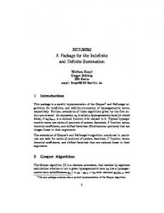
Example (Wilkinson monster []). We perform a simple test of a polynomial equation solver. Consider a polynomial 20
w(x) = ∏(x − j) j=1
in a closed form—we computed the product—and in single-precision floating point representation. en, if we search for the zeros of w(x) with the classical Newton method, we obtain complex-valued solutions. Two plots for the w(x) are shown in Figure .. e reason for such a behaviour of the Wilkinson monster is the inexact floating point representation and the numerical instability of the polynomials. is particular polynomial w(x) has both very large and very small coefficients. us, its representation in floating point system becomes more and more distorted as the computation progresses. e usage of a single-precision arithmetic makes this ̃(x). e polynomials are very instable process more outrageous. Let the distorted polynomial be w ̃ numerically, and the zeros of w (x) differ from the zeros of w(x) to the extent that the former are complex and the latter are not—by construction. What we in fact desire to obtain are methods for the exact computation. We call them from now on ‘symbolic methods’ and consider them as an opposite of the numeric methods. However, the latter can and will serve as a ‘guide’ (in many senses) for our approaches. Still, numeric and symbolic computing methods differ. To give an example: it is very hard to compute Gröbner bases [Buchberger, , Becker et al., ] with floating point numbers [Sasaki and Kako, ]. As symbolic methods are much more resource-demanding than numeric ones, parallel symbolic computing is a highly important research direction. Let us perform a practical experiment. Start Maple [Redfern, , Monagan et al., ], we took the version , available at Faculty of Mathematics and Computer Science at Philipps-Universität Marburg. Generate a large random matrix over rational numbers with(LinearAlgebra): A := RandomMatrix(100, 100, generator = rand(-99..99) / rand(1..99));
and compute its determinant Determinant(A);
It took us . seconds on an -core machine sakania, until the full result was computed. Admittedly, it is a quite large fraction, as we demanded the exact result. However, we observed that while the computation was in progress, only one core of our mighty -core machine was in fact computing the
2
Chapter . Introduction 2.5e+12 2e+12 1.5e+12
w(x)
5e+16 4e+16
w(x)
3e+16
1e+12 5e+11 0 -5e+11 -1e+12 -1.5e+12
2e+16 1e+16 0 -1e+16 -2e+16
6
7
8
9
10 11 12 13 14 15
18.8 19 19.2 19.4 19.6 19.8 20 20.2
Figure .: e Wilkinson monster: the polynomial w(x). Note the amplitude of the values.
determinant, the remaining cores were idle. So, if we could occupy these idle cores too, we would not need to wait almost one and a half minute for the result. We have seen that the parallelisation is very important for computer algebra methods. We will consider a radically different method of computation, namely a residue-based rational arithmetic, in Chapter . We will revisit the Maple determinant computation example on pages –. We will also consider existing algorithms of computer algebra and search for a generalisable high-level parallelisation techniques for these algorithms. We work in the research parallel language Eden [Loogen et al., ], which enables us to use Haskell [Peyton-Jones, ] for specifying both the parallelisation methods and the code to parallelise. We will use ad-hoc polymorphism, higher-order functions, futures and further features of our target language. Our high-level approach will add such benefits as good abstraction from unneeded details and high productivity of the developer to the performance increase drawn from the parallelisation. Our goal is to uncover parallel processing approaches and techniques. We hope that some day, a parallel computer algebra system will emerge which will have utilised this knowledge to become faster. is would serve for the benefit of anyone who has ever been staring in the monitor, waiting for the computation to finish.
Related Computer Algebra Systems Various (sequential) computer algebra systems exist. An overview is in [Grabmeier et al., ]. First systems include Macsyma [Martin and Fateman, ], Reduce [Hearn, ], Axiom [Bronstein et al., ], see also [Davenport, ]. Standard commercial systems nowadays are Maple [Redfern, , Monagan et al., ] and Mathematica [Wolfram, , ]. More special open source systems include CoCoA [Capani and Niesi, , CoCoA, ], GAP [GAP, ], GiNaC [Bauer et al., , GiNaC], KANT V [Daberkow et al., ], PARI [Batut et al., ], Singular [Greuel et al., , Decker et al., ]. An open source bundle of available free systems with a Python-based ‘glue’ to hold them together is SAGE [Stein and Joyner, , Stein et al., ]. Approaches towards parallel computer algebra as a complete system include PARSAC [Kuechlin, ] and PACLIB [Schreiner and Hong, , Schreiner, ]. MuPAD [Naundorf, ], Macaulay [Eisenbud, , Grayson and Stillman, ] and Cannes/Parcan [Gloor and Muller, ] feature SMP support using threads in an otherwise sequential system. is is a low-level approach. An early approach to parallel Maple is [Watt, ]. ere are also techniques to separate parallel orchestration from computer algebra implementation, see, e.g., ∥Maple∥ [Siegl, ], Distributed Maple [Schreiner et al., ], SCIEnce Project [Hammond et al., , SCIEnce, ].
.
Parallel Programming
Parallel programming, a large problem field in computer science, has gained much attention over the last few years. It is considered a new, important front line of the research due to the current trends of computer hardware development [Geer, , Hill and Marty, ]. For a few years now chip makers have been not able to scale CPU performance by increasing speed of a single core. e only recourse is to maintain existing—and needed!—performance growth is to increase the number of processors on a single chip. is still reflects the Moore’s law formulation for the number of the transistors on the same
.. Parallel Programming
3
die [Moore, ], but should the current development continue, we will face thousands of cores on a single die [Agarwal and Levy, ]. However, parallel programming has some caveats [Skillicorn, , Foster, , Grama et al., ]. It is much harder than its sequential counterpart. We need to take care of data partitioning, communication and synchronisation issues. Deadlocks are possible. Good speedups depend on many factors. It is hard to foresee the behaviour of a parallel program for further input sizes or number of processing elements. We want to combine complicated algorithms and (hard) parallel programming. is requires highlevel, abstract, generic programming schemes [Charles et al., , Chamberlain et al., ]. We aim for language-independent techniques. Possible techniques include i) algorithmic skeletons [Cole, ], ii) data parallel approach [Grama et al., ], iii) actors [Hewitt et al., , Haller and Odersky, ], iv) a monad for deterministic parallelism [Marlow et al., ], v) soware transactional memory [Harris et al., ], vi) communicating sequential processes [Hoare, , Abdallah et al., ]. is list includes both approaches towards concurrency and parallelism. We do not assess all of them equally detailed. We concentrate our interest on the parallel methods. We aim to model mathematical algorithms with as few side effects as possible. • e main focus of this work is set on algorithmic skeletons. Skeletons capture parallelisation schemes and communication patterns. ey provide a more formal framework for program construction [Gorlatch, b, Rabhi and Gorlatch, ]. With skeletons it is possible to reuse the most complex part of a parallel algorithm: its parallelisation. Skeletons are oen used in parallel functional languages, as they can be encoded as higher-order functions in this setting. ese properties of algorithmic skeletons make them best candidates for a high-level parallelisation of multiple (formally stated) algorithms, divided in groups, sharing the same paradigm—exactly the context of this thesis. With skeletons we aim to save much effort for the parallelisation of the algorithms in our application area. • We will use the data parallel paradigm from the point of view of algorithm transformations. We search for a better suitable arithmetic, which would limit the intermediate expression swell and enable parallelisation. is is a mathematical technique, which is easily applicable for the problems in computational mathematics. However, it is not a general parallel processing method. Our data parallel approach—aer the algorithm transformation is done—would still require a skeleton to implement the obtained parallelism. ough there are techniques to flatten nested data parallel programs [Blelloch, , Chakravarty et al., ], and thus to make data parallel approach more widely usable, we do not see such techniques to be versatile enough. We search for mathematical techniques to transform algorithms to data parallel representation and do not use nested data parallelism. • We will also briefly discuss actors [Hewitt et al., , Haller and Odersky, ]. e typical actor approach is very different from ours. We will see in Chapter how it is possible to model actors in a high-level manner in the setting of a lazy functional language. Actors are an approach to concurrency, however, we will model them in a parallel setting. • e approach of [Marlow et al., ], the deterministic Par monad, confines all the implementation in a monad. Our algorithmic skeletons would require the sequential code to use the (sequential) higher-order functions, which will be then replaced by skeletons. Par requires all the code to be monadic, which is a larger transition. Further, the preliminary measurements show [Marlow et al., ] that the Par monad is in most cases significantly slower than traditional Multicore Haskell [Marlow et al., ]. erefore, we do not consider this approach to parallelism in more detail. • A rather high-level approach to concurrency is soware transactional memory (STM). First publications on this topic are [Knight, , Herlihy and Moss, ], see also [Shavit and Touitou, , , Harris et al., , Herlihy, ]. e basic idea is that transactions for memory access either succeed or fail. In the latter case, the STM implementation just tries again, until
4
Chapter . Introduction success is reached. It can be used for lock-free data structures. STM is quite accepted in the industry, cf. [Adl-Tabatabai and Shpeisman, ], furthermore it can be nicely implemented in Haskell [Peyton-Jones, , Harris et al., , O’Sullivan et al., ]. STM can also be used to fix some possible inconsistencies [Bieniusa et al., ]. In our view, using STM for our aims has multiple drawbacks. Firstly, STM can be used only in the shared memory setting. We aim for techniques usable both in distributed and in shared memory settings. Networks of multicore machines need both approaches [El-Rewini and AbdEl-Barr, ]. Secondly, it is not a very high-level approach. STM can free the programmer from locking, but it still enforces a quite low-level programming model, involving transactions and atomic blocks. e third reason is the same as with Par monad: Haskell’s implementation of STM is monadic. Hence, we will need to majorly restructure sequential code to use STM. And the most important reason is: STM is an approach for concurrency, not for parallelism. Contrarily to actors, we see no easy way to implement STM in the parallel functional setting. We do not regard STM in further, focusing on parallel high-level methods. • e communicating sequential processes [Hoare, , Abdallah et al., ] is a quite formal approach. In fact, it is a calculus for concurrency. Implementations include [Jones and Jones, , Brown and Welch, , Welch and Barnes, , Brown, ]. We do not consider this model here. e reasons are twofold. Firstly, it is an approach towards concurrency. Contrarily to this fact, we focus on the parallel computing, as detailed above. Secondly, available Haskell implementation is monadic, hence we have similar drawbacks as in Par monad and STM.
.
Goals of is Work
We aim to answer the following question. Whether and how can we utilise high-level approaches for the efficient parallelisation of the core algorithms of computer algebra? Can we extract skeletons from common computer algebra algorithms? How do we make the symbolic computation possible in the chosen setting? Which skeletons do we need to implement? How can we ensure portability and reuse of our work? Are we able to apply the above mathematical technique not only in theory? How can we model actors in our setting? is thesis proceeds in two directions towards the answers to these questions. Firstly, we contribute high-level parallelisations for some popular problems in computer algebra. Secondly, we introduce further evaluation methods, see below.
..
Parallel Symbolic Computation
• We require basic support for symbolic computations, i.e., a way to express computer algebra algorithms independently from concrete underlying algebraic structure. To give an example: not ‘polynomials over Z’, but ‘polynomials over a unique factorisation domain’. is thesis will present our approach to this issue. We need to represent values of arbitrary size, and not only the ones fitting in some hardware registers: unsigned hardware integers are bounded with 264 on bit hardware. We require an implementation of fractions. It is possible to represent them as pairs of integers. However, we embark on a different route. We will present an alternative approach to the representation of fractions, which maps well to a parallel processing paradigm. We need to represent not only rationals, but also irrational values exactly. e algebraic method is adjunction. With it we add the needed irrational value symbolically to the number system we work in. We will present our implementation of adjunction in this work.
.. Structure of e esis
5
• We contribute skeletons for parallel polynomial and integer multiplication. Our approach is to parallelise fast divide and conquer methods. We are interested in both Karatsuba multiplication and in methods based on the fast Fourier transform. e latter account for the complexity of the multiplication being O(n log n) for the polynomials of degree n, provided some limitations hold. e consequence is: we implement the parallel fast Fourier transform. As it is also a divide and conquer algorithm, we will investigate to what extent it is possible to share a single divide and conquer skeleton between such very different algorithms. • We contribute approaches for parallelising matrix multiplication and decomposition. We parallelise the fast matrix multiplication algorithm by Strassen [] (again a divide and conquer algorithm!) and the LU decomposition of matrices (also known as Gauß elimination). An important application of the latter is the determinant computation. • In some algorithms of computer algebra, e.g., in Gauß elimination, naive polynomial GCD, Buchberger’s algorithm, a very fast increase of the rational entries in the mathematical structures occurs. Examples are coefficients of polynomials for GCD and Gröbner bases, and entries of the matrices for Gauß elimination. Such growth is called intermediate expression swell [Tobey, , von zur Gathen and Gerhard, , Brickenstein, ]. We require a method to prevent the intermediate expression swell—and to do so in parallel. We contribute a residue arithmetic for this goal. We present approaches for both integers and rationals. Further, it should be possible to compute with the residue arithmetic in parallel. An apparent approach is to use multiple residue classes a in data parallel manner. Some questions arise. It it correct? Residue classes are well known for the integer residues. How can we tackle fractions? Is it possible to use multiple residue classes for fractional residues? We will answer the above questions in this thesis. e approach towards a fractional multiple-residue arithmetic is the result of our long-term research. • For the residue arithmetic we implement methods to find quite large primes. Even leaving the residues aside, primality testing is a very interesting and required discipline. Not least this is so because of public key cryptographic systems like RSA [Rivest et al., ], which require large prime numbers. We will abstract the parallelisation patterns (i.e., the skeletons) for probabilistic primality tests. We will also discuss and evaluate the performance of these methods.
..
Evaluation Methods
Secondly, aer obtaining some results for the performance of our new-craed implementations on the hardware available to us, we contribute methods to to i) evaluate thoroughly these results, ii) find and apply an approach to generalise these results. is means, we contribute • A method to predict the execution time of a given program for non-measured input sizes and for non-measured numbers of processors. • An ability to verify the quality of a parallel implementation quantitatively. We apply it to the parallel programs we will present.
.
Structure of e esis
e remaining text is structured as follows. Chapter discusses the choice of a lazy functional programming language for the implementations in question. We also introduce the language unity approach in Chapter . Chapter presents the parallel functional language Eden [Loogen et al., ], which is well suited for the development of the skeletons in the further chapters. We will see in further chapters why some features of Eden are essential for this thesis. Chapter presents the methods for the estimation of parallel programs’ run times mentioned above. ese methods are our novel work. We examine
6
Chapter . Introduction
the probabilistic primality testing methods and develop new skeletal approaches for their parallelisation in Chapter . We consider fast multiplication routines for polynomials, integers, and matrices in Chapter . All algorithms in this chapter are divide and conquer algorithms. We will see how we can reduce the implementation overhead with skeletons. e same chapter features actors. A throughout evaluation is also included. A novel parallel rational residue arithmetic is presented in Chapter . e same chapter also presents an integer residue arithmetic. ese implementations form the data parallel approach. Further, we present there an example using matrix decomposition and evaluate its performance with the new arithmetic. Conclusions, future, and related work follow in Chapter .
C
P R O G R A M M I N G L A N G UA G E S A N D S Y M B O L I C C O M P U TAT I O N
ere is no mode of action, no form of emotion, that we do not share with the lower animals. It is only by language that we rise above them, or above each other—by language, which is the parent, and not the child, of thought. Oscar Wilde, e Critic as Artist
and A.D. Muhammad ibn Mūsā al-Khwārizmī, *c. , †c. , wrote AlKitāb al-mukhtasar fī hīsāb al-ğabr wa’l-muqābala (اﻟﻜﺘﺎب اخملﺘﺼﺮ ﻓﻲ ﺣﺴﺎب اﳉﺒﺮ واﳌﻘﺎﺑﻠﺔ, “e Compendious Book on Calculation by Completion and Balancing”). It features the concepts of al-ğabr and muqābala—the symbolic computation and term reduction. is book’s content and its author’s name are also good known for giving us the words ‘algebra’ and ‘algorithm’ respectively [Rāshid, , Chabert, , Grabmeier et al., ]. Rafael Bombelli (*, †) published Algebra in , introducing rules for computation with complex numbers. John Pell, *.., †.., tabelised in the factors of all integers up to . Leonhard Euler, *.., †.., significantly advanced algebra, number theory, and various other fields of mathematics. Another mathematical genius, Johann Carl Friedrich Gauß, was born ... He proved the fundamental theorem of algebra in . His Disquisitiones Arithmeticae appeared . It features advances in number theory and algebraic constructions. e latter part of this book utilises the complex roots of unity. Gauß died .. [Eves, , Chabert, , MacTutor, ]. John Napier (also: Neper, Nepair) of Merchiston, *, †.., introduced Napier’s bones, a kind of mechanical calculator. Napier is one of the discoverers of logarithms, alongside with Briggs and Bürgi. Edmund Gunter (*, †..) develops Gunter’s scale, a mechanic device capable of multiplication using logarithms, in . is device was the predecessor of a slide rule. John von Neumann (*.., †..) and Norbert Wiener (*.., †..) produced the foundations of contemporary computing hardware. James Hardy Wilkinson, *.., †.., was one of the first scientists to raise awareness towards approximate methods and numeric computing—the finesse of the computation, adapted to the hardware of the digital computers [MacTutor, ]. e symbolic computation in the modern sense, as opposed to the numeric computation, is merely a few dozen years old: various sources state either [Kahrimanian, , Nolan, ] or [Birch and Swinnerton-Dyer, ] as emerging publications on this topic. We generally use the terms ‘symbolic computation’ and ‘computer algebra’ as synonyms, for the fine difference between these concepts see, e.g., [Watt, ]. Symbolic computing is computationally very intensive not only because of the symbolic representation of data, but also because of some negative effects, e.g., intermediate expression swell [Tobey, , von zur Gathen and Gerhard, ]. ese facts motivate the development of parallel computer algebra systems. We will focus on parallel programming languages in Chapter . Here we discuss the (sequential) features of a language for symbolic computation. is chapter will provide the programming language foundation of this thesis. We chose Haskell for our implementation of the algorithms of computer algebra. It is a statically typed lazy functional programming language [Peyton-Jones, ]. We will see below which features of Haskell make it especially suitable for our tasks. e first section discusses the problems, an efficient implementation of a computer algebra system needs to solve. e remaining part of this chapter is organised as follows. Section . discusses the language unity concept. Section . explains the type problems, connected with algebraic domain construction. Section . provides an example of symbolic
B
8
Chapter . Programming Languages And Symbolic Computation
computing with Haskell. It emphasises the importance of laziness. Section . concludes the chapter. We will discuss the details connected with the implementation of parallel algorithms in the next chapter. We assume a good knowledge of Haskell [Peyton-Jones, ], see, e.g., [Doets and van Eijck, , Hutton, , O’Sullivan et al., ].
. Symbolic Computation So, we want to perform a symbolic computation. Systems doing so are called ‘computer algebra systems’, abbreviated CAS. As we move away from floating point arithmetic (and overflowing hardware integer arithmetic), the first step is an arbitrary precision integer arithmetic. However, the cost of a single arithmetic operation with such arithmetic is no longer constant—it depends on the length of the integers. (See Chapter for fast multiplication routines.) e implementations of arbitrary precision integers include the GNU multiprecision library [Granlund and Swox, ] and the CLN library [Haible and Kreckel, ]. Also noteworthy is the NTL [Shoup, ], which, focusing on number theory, begins with implementing the foundations for it. An increasing number of modern programming languages, including Haskell, provide access to an implementation of arbitrary precision integers [Peyton-Jones, , van Rossum, , Flanagan and Matsumoto, , Odersky et al., ]. We can take arbitrary precision integers for granted in these languages. Haskell with its approach to polymorphism is especially convenient. In Haskell the arbitrary precision integers are called Integer, as opposed to the hardware integer type Int. We can use the usual arithmetic operations’ signs: f :: Integer → Integer f x = 10^10000 + x
In the GHC implementation of Haskell the Integer type is implemented with the GNU multiprecision library. In Haskell we can easily manipulate mathematical objects in a manner quite conventional to a mathematician. To give an example, we can define the factorial as product [1..n], which maps very well to the usual mathematical notation. Beyond integers. However, arbitrary precision integers are just a first step to symbolic computing. We require an implementation of fractions, which can be accomplished quite simply using pairs of arbitrary precision integers. Still this aspect is interesting, see the aforementioned packages for elaborate implementation. To give an example, one of the important questions, arising from a traditional implementation of fractions, is ‘when do we reduce?’ Recall, a fraction a/b is called irreducible, when a and b have no common factors. A fraction ka/kb is not reduced, in other words: not in its lowest terms. e irreducibility test involves a computation of the greatest common divisor (GCD), which is quite costly to perform aer each arithmetic operation. On the other hand, not reduced fractions are larger, so further arithmetic operations would be more expensive. But there is a larger problem. We need to represent irrational values in our system. is issue is not present in floating point arithmetic, as it simply uses approximations. e key solution comes from algebra and is well known: it is called adjunction. For the sake of it we switch from rationals to rings of polynomials over rationals, as we will see below. √ √ Example (Adjunction). We want to adjunct 2 to Q. e result is written formally as Q( 2). e technical side is that we compute from now on in Q × Q,√where for the √ second component √ similar rules apply, as for the imaginary part of C. For instance, (a + 2b) ⋅ (c + 2d) = (ac + 2bd, 2(bc + ad)). √ A classic example for adjunction is C, which is in fact R( −1). For the generic adjunction to be feasible on a computer, factor rings modulo the ideal, generated by specific polynomials, are used. ese polynomials have roots, which are √ exactly the values to adjunct, and these polynomials are irreducible¹. So, if we want to represent Q( 2), we use in fact Q[x]/⟨x 2 − 2⟩. In Section .. we will ¹For the definition of irreducible polynomials see Definition A. on page in the Appendix or any algebra book.
.. Language Unity
9
see more on how to work with such polynomials. Such an approach accounts for the infamous RootOf expressions in computations, using CAS. We consider √ polynomials (as well as other mathematical structures) over an arbitrary field F. So, F could be Q( 2), but we actually do not care, as we simply construct F[x] over it. is is one of the meanings of symbolic computation: we abstract from the representation of base elements of our structures. is is our principal approach throughout the thesis. For the sake of completeness, the other meaning is the possibility to introduce symbols. We do not discuss the latter side of symbolic computing in detail. Our approach, elaborated below, provides these features for free. As we have indicated before, symbolic computations take more resources into account than numeric ones. is lies partially in the nature of the algorithms used. Partially, the data representation is at fault. If we work in Q[x]/⟨ f ⟩ with an irreducible polynomial f of degree n, then we have up to n times more work, as compared to a computation directly in Q. A parallelisation can provide capacity to deal with such an increasing workload. We will see in Chapter how to implement adjunction in Haskell. Other caveats. But even an efficient implementation of Q is not a silver bullet! Some algorithms, like naive polynomial euclidean algorithm, Gauß elimination, or Buchberger’s algorithm, suffer from so-called intermediate expression swell [Tobey, , von zur Gathen and Gerhard, , Brickenstein, ]. is means that the intermediate expressions grow very fast. is growth is stimulated by the fact that small-valued fractions might still be large expressions. For instance, 9999999999 10000000000 is a very small fraction, near to 1. However its representation is quite large. ere are a few workarounds. We can divide them into two approaches. Firstly, we can use another arithmetic. is is a quite generic technique, Chapter elaborates on our approach, the residue-based arithmetic. Further possible methods include some other residue-based approaches, arbitrary precision floating point numbers [Priest, ], and continued fractions [Perron, , Khinchin, ]. While all residue classes pursue the same goal with likely methods, which method is better is a vast topic for research. However, any residue arithmetic requires an upper bound on the final result. e two other approaches are unfortunately unsuitable here. Arbitrary precision floating point number systems should be prescaled to a desired size. An expert is needed to choose the required size. ere is some work on adaptive, self-scaling arbitrary-size floating point arithmetic [Shewchuk, ], but in practise problems with rounding in the hardware floating point numbers can arise. As for continued fractions, they have very suitable properties for representing rational values and even approximations to real values. But actually computing with continued fractions is a rather hard task. Secondly, in some cases, e.g., in a polynomial euclidean algorithm, we do not particularly need exact representation of all coefficients of intermediate polynomials, an approach pioneered by Lehmer []. Methods using a similar idea belong to the area of symbolic-numeric computing. Great success has been achieved, e.g., in the acceleration of the LLL algorithm [Koy and Schnorr, , Nguyen and Stehlé, , Stehlé, ]. We do not elaborate on this approach here. Symbolic algorithms. Another feature our target programming language should support is an ability to express generic symbolic algorithms. To give an example, an implementation of polynomials R[x] should work fine, regardless of which base unique factorisation domain R is currently used. We will see in Chapter how Haskell’s type system, especially type classes, help to implement symbolic computation.
.
Language Unity
In this section we generally follow [Lobachev and Loogen, ]. e problems the programmer of a computer algebra system (CAS) needs to solve are hard [Cohen, , von zur Gathen and Gerhard,
10
Chapter . Programming Languages And Symbolic Computation language internal external implementation efficient compiled static
interaction comfortable interpreted dynamic
Table .: Two languages of a CAS.
, Grabmeier et al., , Ribenboim, , Levandovskyy, ]. For that, an expressive programming language with high-level concepts is desired. But the actual situation with programming languages of a CAS is more difficult. A CAS is a large piece of soware, and it is implemented efficiently in a particular programming language. We call this language an internal language of the system. It is desired to be fast, which comes not without a price. However, the users of the system would like to program. Even more, since the users want to express mathematics in their programs, they would be happy to find matrices, polynomials, symbolic integration etc. predefined. By ‘predefined’ we mean here either in a standard library or as a primitive. It is not important for us, which one. For these reasons, a second, external or interface language is introduced. e internal language should be safe and fast, we imply it has a good compiler and a static type system. e external language should be able to embrace all the mathematics the user may want to express. It seems desirable to choose a dynamic language. It will be embedded into the ‘actual’ CAS implementation. e external language needs to express the whole spectre of mathematical structures and their relations. e drawbacks include: • Some low-level features, e.g., file access, might be missing in the external language. • e external (interpreted, dynamic) language might be orders of magnitude slower than the internal (compiled, statically typed) one. • Two possibilities exist for the implementation of the external language. – It is implemented in the internal language. In this case we need to implement support for all the features of the interface language in the efficient, but low-level internal one. ink of implementing LISP in C as a by-project! Our aim is not to write a compiler or an interpreter. – e other option is to take an off-the-shelf embeddable language, like Groovy [Barclay and Savage, ] or any other small dynamically typed language, like Python [van Rossum, ] or Ruby [omas et al., , Flanagan and Matsumoto, ]. In fact, Python is used as glue between the programs in SAGE [Stein and Joyner, , Stein et al., ]. For both approaches towards the implementation of an external language, we need to provide access to the core functionality, implemented in the internal language, to the external language programmers, cf. R [Ihaka and Gentleman, , R Development Core Team, ], where the internal language is C and the external one is a Scheme-like language. is is less of an issue. But it makes impossible for the user to ‘look into’ and to modify some core functionality: at some point the correct answer on the question ‘how is that defined?’ becomes ‘it is a hook to a function in a bundled internal language library.’ e requirements to both languages are briefly sketched in Table .. Fortunately, there is a solution. An interesting approach was done by the developers of GiNaC [Bauer et al., ]. is system is written in C++ and has C++ as its interface language. is is exactly the approach we aim to implement. is way, not a computer algebra system, but rather a computer algebra library emerges. In other words, we do not create a new system with required features, both programming-language-wise and computer-algebra-wise, but rather extend a given programming language by computer algebra features. In this work we focus on algorithms. Hence, we
.. Dependent Typing Language
C
Efficient Compiled Interpreted High-level ADT HOF Statically typed Type inference
✓ ✓ ✓ ? ✓
Python ? ✓ ✓ ? ?
11 Haskell ✓ ✓ ✓ ✓ ✓ ✓ ✓ ✓
Table .: Features of CAS languages in the mainstream.
would include in our library some types and functions for expressing certain computer algebra algorithms. We consider the types only as far as needed for the algorithm implementation. To give an example, we would implement a type for a univariate polynomial over another, given type. But we would not implement a type for an arbitrary skew field. Getting back to GiNaC, its implementers had to overcome a rather large problem. e C++ language is a compiled one. But a typical CAS interaction is not only a batch job for some finely written code execution! It is also a long interactive session for finding the particular fine code for a given problem. Can GiNaC be used for that? e answer is yes. Although a C++ interpreter exists, the library implementers chose another way: GiNaC provides its own interactive interface. It is not complete, but it is usable. Are we back at external language design, despite all our efforts? No! e conclusion we draw from the GiNaC case is: the desired implementation language should possess both a compiler for efficient execution of batch jobs and an interpreter for interactive programming sessions. Having these and adding the CAS-as-a-library idea, we obtain the language unity concept, elaborated in [Lobachev and Loogen, ]. is paper pushes the idea further: this common language for both implementation and interaction of the CAS library should be a statically typed functional language, cf. Table .. e latter compares C [ISO/IEC :], Python [van Rossum, ] and Haskell [Peyton-Jones, ]. e question mark in the table means that some approach exists, but it is not a mainstream implementation. Further, ADT stands for algebraic data types, and HOF stands for higher-order functions. We consider such features essential for a CAS development. Let us discuss the table in more detail. Results on efficiency of various languages’ implementations and on programmer’s productivity are available in, e.g., [Hudak and Jones, , Fulgham and Gouy, ]. We are not aware of a full Python compiler which would produce machine code. All approaches known to us focus on just-in-time compilation. A mature interpreter for Haskell is GHCi, further implementations exist. ere are some approaches to higher-order functions in Python, but they are not the main focus of the language. Similarly, it is possible to use functional pointers in C to represent higher-order functions, but we would refrain from such dangerous constructs. is is a common industry practise [Hatton, ]. C is statically typed, but it has no type inference. Another benefit of a CAS library is the availability of language constructs for the user: name binding in the interface language provides the symbol manipulation for free. We will see in following, how we can implement the symbolic computation, i.e., an abstraction from the representation of base elements.
.
Dependent Typing
ere is a known problem with expressing algebra in a typed functional language. If we define a separate type for each kind of algebraical structure, then we promptly find out that the type of some further algebraical structure depends on its properties. Or, in programming language terms: the type depends on the properties of the value of this very type.
12
Chapter . Programming Languages And Symbolic Computation
Example .. Suppose we have some n ∈ N and build a residue ring Z/n. e notation is n = ⟨n⟩ = nZ for an ideal n, generated by n. We cannot state if the ring is a field or not, without examining the fact whether n is prime. However, in a Haskell definition of residue rings: residueRing :: Ring → Ideal → Ring residueField :: Ring → Ideal → Field
the second definition is wrong. As not every residue ring is a field, the matter whether it is one, depends on the properties of a specific value of Ideal. Such problems were described in the works of Serge Mechveliani [Mechveliani, , a,b]. One possible solution is dependent typing. But as we focus on algorithms and their parallelisation, this problem is not acute for us. We do not actually want to represent the hierarchy of algebra constructs, but to implement some algorithms! A full-grown implementation should rather use a dependently typed parallel functional language. However, in our prototype we resort to a Hindley–Milner typed (parallel) functional language. (Aer J. Roger Hindley, * and Robin Milner (Arthur John Robin Gorell Milner), *.., †...) See [Hindley, , Milner, , Damas and Milner, ] for the Hindley–Milner type inference algorithm. e only approach to a parallel dependently typed language known to us is parallel Aldor [Gautier and Mannhart, , Maza et al., ].
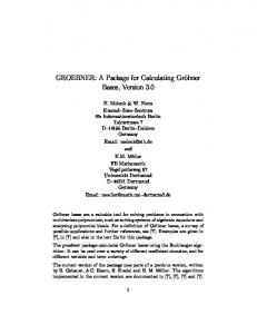
. An Example: Laziness Why is laziness important in a programming language for symbolic computation? A lazy, non-eager evaluating programming language can be used to represent mathematical objects in a more natural manner, see [Karczmarczuk, , Hinze, ]. We will see in the course of this work how lazy semantics can be used to express both computer algebra algorithms and parallelisation in a more easy manner. For an example of the latter see Chapter . In this section we will present a very elegant ‘toy’ example for lazy evaluation in a mathematical context. Further cases will be presented in the course of this work. Power series. Closely following [McIlroy, , ], we present some operations on power series encoded in Haskell. We define power series as an infinite list of coefficients. e required basics are in Figure .. It defines the Num and Fractional instances for (infinite) lists. We reiterate, we assume the reader knows Haskell. Having these basics we can easily write Haskell code for some basic calculus operations, like derivation and integration. deriv :: (Num a) ⇒ [a] → [a] deriv (f:fs) = helper (∗) fs 1 deriv _ = [] integral :: (Fractional a) ⇒ [a] → [a] integral fs = 0 : (helper ( / ) fs 1) helper :: Num a ⇒ (t → a → b) → [t] → a → [b] helper op (g:gs) n = g‘op‘n : (helper op gs (n+1)) helper _ _ _ = []
Note, helper is a higher-order function. As soon as we have integration, we can define the series expansion of the exponential function. -- exponential function expx :: [Rational] expx = 1 + (integral expx)
.. An Example: Laziness
13
default (Integer, Rational, Double) infixl 7 .∗ (.∗) :: (Num a) ⇒ a → [a] → [a] x .∗ (y:ys) = x∗y : x.∗ys _ .∗ _ = [] instance Num a ⇒ Num [a] where (+) = zipWith (+) -- all lists are infinite (-) = zipWith (-) (x:xs) ∗ g@(y:ys) = x∗y : (x.∗ys + xs∗g ) _ ∗ _ = [] fromInteger x = (fromIntegral x) : repeat 0 instance Fractional a ⇒ Fractional [a] where (0:xs) / (0:ys) = xs / ys (x:xs) / (y:ys) = let q = x / y in q : (xs - q.∗ys) / (y:ys) _ / _ = []
Figure .: Some initial code for encoding power series in Haskell. We base our presentation on [McIlroy, , ].
We can also easily define some recursive number sequences, like Catalan numbers. Note the arbitrary precision integers. catalan :: [Integer] catalan = 1 : catalan^2
Mutually recursive definitions are also not a problem: we define sine and cosine expansions in a very concise manner. sinx, cosx :: [Rational] sinx = integral cosx cosx = 1 - (integral sinx)
Of course, we cannot compute the complete series in a finite time, but these potentially infinite, mutually recursive and complex definitions result in the correct output—without a failure. We merely need to request some, but not all coefficients of the power series. Note, that the same definition of power series was used both for integers and rational numbers. is is the ad-hoc polymorphism. We will discuss it later, in Chapter . We can verify the correctness of McIlroy’s approach with the QuickCheck library. e definition of the test for the definition of cosine with the well-known identity sin2 x + cos2 x = 1 is below. test :: Int → Bool test n = let cs = take n $ sqrt $ 1 - sinx^2 in cs == take n cosx
Powering roots of unity. Another example of laziness in our main codebase is the generation of the powers of roots of unity in Chapter . Let us not bother now, what exactly is a primitive root of unity. Let us assume, it is already defined as w somewhere in our program. en we can generate all powers of it with ws = map (w ^) [0..]. is corresponds well with the mathematical notation ω = [ω0 , . . . , ω n ] for some n ∈ N. In the contrast to the latter, we denote all powers of ω. But indeed only the values really required in the subsequent computation will be generated. So, if we need only n/2 powers of ω, we will generate exactly that many. No action is required to save work.
14
Chapter . Programming Languages And Symbolic Computation
Conclusions. We can model some advanced mathematical structures in Haskell with ease and grace. We do not use power series in the further text, but the second example is a clear part of our work. We rate laziness as one of the most important Haskell’s features. Lobachev and Loogen [] presented further examples and compared the speed of Haskell and C++ in one of the case studies.
. Conclusions and Outlook Haskell is very suitable for implementing computer algebra algorithms. Our ‘language unity’ approach tells us we should use Haskell as both implementation and interface language of a computer algebra system. We conclude that build-in arbitrary precision integers and lazy evaluation can be very useful for implementations of symbolic algorithms. We have seen how easy it is to define differentiation and integration in terms of infinite power series in Haskell. One more feature we will use in the next chapters for the implementation of computer algebra algorithms is the ad-hoc polymorphism. Haskell is a very expressive language, so we can use the abstraction techniques for a generic programming approach. One of the most important features of Haskell are higher-order functions. e functions are first class citizens in Haskell. We will use higher-order functions to represent algorithmic skeletons. In multiple aspects Haskell is a very ‘mathematical’ language. As mentioned above, list comprehension syntax in Haskell has an almost one-to-one correspondence with the set notation in mathematics. is is of a benefit for our implementation. We will consider the parallel lazy functional language Eden in the next chapter.
C
PA R A L L E L P R O G R A M M I N G W I T H E D E N
e tale is old as the Eden Tree— as new as the new-cut tooth. Rudyard Kipling, e Conundrum of the Workshops
we have seen in the previous chapter, we need to use a statically typed functional programming language. We aim for a parallel computer algebra implementation, so we also need a support for parallelism. Section . has shown that laziness is of benefit to express mathematics in a programming language. We will see in this thesis that laziness is also of benefit to represent parallelisation concisely. In the following, we use a parallel lazy functional language with explicit process creation. Such a language, based on Haskell, is under development in Marburg and Madrid and is called Eden [Loogen et al., ]. With it we can focus on the development of the algorithmic skeletons for computer algebra algorithms, which is the actual subject of this thesis. Our choice of Eden is influenced by the following features:
A
• Eden is a language with explicit parallelisation. us we will always have exact control of what is exactly executed in parallel [Loogen et al., ]. • Eden has a large skeleton library with sophisticated skeletons, implemented in Eden itself [Loogen et al., , Eden Skeletons, ]. • ere is a possibility of dynamic communication in Eden [Breitinger and Loogen, , Berthold and Loogen, , Dieterle et al., b]. • Eden features futures [Dieterle et al., b] and process network construction tools [Horstmeyer and Loogen, ]. • Eden performs well both on distributed memory machines and on shared memory multicores, see e.g., [Berthold et al., a]. • It is easy to express high-level parallelism in Eden [Loogen et al., , Berthold and Loogen, , Berthold et al., b]. ere are multiple approaches to a parallel Haskell. We chose Eden as it gives us the most control of the parallelisation, but without bothering us with unneeded, low-level details, in contrast to Haskell+MPI. We will present alternative approaches to parallel Haskell in Section ... Structure of this chapter. In Section ., we describe Eden and determine its position in terms of classifications, which we will present below. en we review existing approaches to parallel computing in the context of Haskell programming language in Section ... We describe the process model of Eden and an important extension of the language in Sections ..–... In Section .. we review the drawbacks and benefits of lazy evaluation in a parallel setting. Section . presents a survey of existing algorithmic skeletons implemented in Eden. Some helper functions for list manipulation are also defined there. Further, Section . introduces the Eden TraceViewer and the whole concept of tracing, whereas Section . discusses hardware, conventions and approaches we use to measure the parallel execution time of our programs. Section . concludes the chapter. We present two taxonomies of parallel processing next, Flynn’s and Foster’s approaches. We will apply them to Eden and other parallel Haskells next.
16
Chapter . Parallel Programming With Eden Instruction single multiple Data
single multiple
SISD SIMD
MISD MIMD
Table .: e Flynn taxonomy.
Flynn taxonomy. e classic taxonomy of parallel computing by Flynn defines the matrix of single/multiple ‘instructions’ on separate nodes and of single/multiple data streams [Flynn, ]. ese are abbreviated, e.g., ‘single instruction, multiple data’ becomes ‘SIMD’. e Flynn taxonomy results in four possible combinations, as shown in Table . [Grama et al., ]. e classic sequential computing is SISD. e ‘vector’ machines realised the SIMD principle. Independent computers working on different data with various methods obey the MIMD scheme. e extension of the taxonomy considers not the particular hardware instructions, but rather the complete program codes. An example would be SPMD. PCAM Methodology. Foster [] defines four different stages of the development of an efficient parallel algorithm. ese stages are noted aer their first letters as PCAM: partitioning, communication, agglomeration and mapping. e partitioning stage consists of domain decomposition and functional decomposition and designates separate tasks for the parallel processing. ere are some recommendations on the number of tasks (e.g., at least an order of magnitude more than processing elements), granularity of tasks, scalability of the partition. In the communication stage locality and structure of the communication are considered. For instance, we might consider reordering the data so that one-to-one communications happen more oen between neighbour processing elements (PEs). Furthermore, it is important that one-to-many (many-to-one) schemes do not exceed the bottleneck of the single sender (receiver). Another point of consideration is dynamic communication. Here the communication channels are not established beforehand, but are created while the computation is already in progress. Finally, asynchronous communication is possible. Foster [] underlines the importance of it in a distributed memory setting. Agglomeration stands for merging small tasks from the partitioning stage to larger tasks. An important aspect of agglomeration is to merge interdependent tasks together and to reduce the need in communication. en, mapping designates where each task has to be executed. In this phase the tasks are assigned to processing elements, it is so called ‘process placement’. e optimal mapping problem is N P-complete [Bokhari, ], but there are some specialised heuristics and strategies for particular cases. One of the approaches to mapping are various methods of load balancing, see, e.g., [Tantawi and Towsley, , Foster, , Kwok and Ahmad, a,b]. e load balancing methods include both some partitioning approaches, like graph partitioning and round-robin balancing, and task scheduling approaches, like various master-worker schemes, including more sophisticated hierarchical and distributed master-worker implementations [Hamdi and Lee, , Shao et al., , Shao, , Aida et al., , Grama et al., ]. Eden-based master-worker schemes include [Peña and Rubio, , Loogen et al., , Priebe, , Berthold et al., , Dieterle et al., a]. Language classification. We distinguish between the work done by the compiler or by the runtime system and the work done by the programmer. In Table . we show classification of parallel languages based on PCAM. We show a dash (–) if a stage is completed by a compiler or a runtime system (RTS). We show the letter if an appropriate stage has to be done manually.
. Eden as Haskell Extension Commonly developed at Philipps-Universität Marburg and Universidad Complutense de Madrid, the lazy parallel functional language Eden [Loogen et al., ] is a programming language with an explicit
.. Eden as Haskell Extension
17
Language
Implicit
Semi-explicit
‘Control’
Explicit
Approach Stages
Data Parallel
Annotations P
Process control PCA
Full PCAM
Table .: Classification of parallel languages.
process instantiation but implicit communication. e classification of Eden aer the extended Flynn taxonomy is SPMD. In the PCAM classification, Eden is PCA. Basing on these classifications, we consider Eden to be a ‘control’ parallel language. As we shall see in following sections, we have explicit process control and an option for explicit communication. In contrast, GpH [Trinder et al., ] is an annotation-based language. We discuss details and further approaches in the next section. We assume the knowledge of Haskell. Still, we will detail on usage of library functions and important utilisations of laziness in the following. Eden has been implemented as an extension of the Haskell compiler GHC. e extensions include minor modifications of the parser for dynamic channels (see below), a few additional ‘ways’ of compilation and a special parallel runtime. e parallelism is organised as follows. e runtime provides special parallel primitives [Berthold and Loogen, a], mostly implemented as function calls to an underlying parallel middleware. Currently MPI [Snir et al., , MPI, ] and PVM [Sunderam, , PVM, ] are used. An option to use direct memory copy is in work [Pickenbrock, ]. e mentioned primitives form a basis for higher-level language constructs [Berthold, ]. We aim to use some low-level skeletons in the higher-level ones, cf. ‘implementation skeletons’ [Klusik et al., ]. As we regard Eden from the application programmer’s point of view, it suffices to give denotational overview of higher-level Eden constructs. Various aspects of the Eden semantics have been studied in, e.g., [Breitinger et al., , HidalgoHerrero and Ortega-Mallén, , , Sánchez-Gil et al., ].
..
Flavours of Parallel Haskells
Pure functional languages are seen as quite a tempting base for a parallel language. e reason for this lies in the fact that the order of reductions is irrelevant in a pure functional language. For example, given two functions f and g, if a function f neither consumes output of the function g nor vice versa, then the applications of these two functions can be evaluated—reduced to head normal form—simultaneously. As Haskell is a mature pure functional language, quite a few attempts have been made for a parallel Haskell. An overview is in [Trinder et al., ]. A seemingly abandoned pioneer is H [Aditya et al., , Nikhil and Arvind, ]. At roughly the same time Haskell+MPI was researched [Breitinger et al., , ]. A recent development is [Astapov et al., ]. e desire to explicitly control the process creation resulted in Eden, one of the first publications was [Breitinger and Loogen, ], the standard reference is [Loogen et al., ]. Eden has been designed as a distributed memory language; however a threaded simulation is available [Breitinger et al., ]. Even more, we found that the standard, distributed memory implementation of Eden performs surprisingly well on the multicores [Berthold et al., a]. A version using directly communicating OS processes on multicores is being developed [Pickenbrock, ]. Eden is implemented basing on GHC, the Glasgow Haskell compiler. Quite a different approach to parallelism is the implicit process control. It falls under the P category of the PCAM classification. In Haskell this approach is implemented in GpH language [Trinder et al., ]. It carries out parallelism with evaluation strategies and annotation combinators [Trinder et al., a]. Two different implementations exist for the language GpH. GpHGUM [Trinder et al., b, b, ] is a virtual shared heap implementation for the distributed memory machines, it is a fork of GHC. Multicore Haskell [Marlow et al., ] is implemented as an SMP language on top of GHC. Both Multicore Haskell and Eden threaded simulation [Breitinger et al., ] utilise for their implementation the same concurrency primitives of GHC—the Concurrent Haskell [PeytonJones et al., ]. At the same time, Eden and GpHGUM share a part of their code base in the
18
Chapter . Parallel Programming With Eden
implementation of a parallel runtime system [Berthold, ]. However, the explicit process control of Eden shows its benefits in comparison with both implementations of GpH [Loidl et al., , Berthold et al., a]. Recent developments include the Par monad for deterministic parallelism [Marlow et al., ] and Cloud Haskell [Epstein et al., ]. e latter is quite similar to Erlang [Armstrong, ]. We discussed Par briefly in Chapter . A completely different approach is Data Parallel Haskell [Chakravarty et al., ]. It implements support for distributed arrays and utilises a special transformation layer to flatten nested data parallel loops. It this sense it is similar to NESL [Blelloch and Greiner, , Blelloch, ].
..
Eden Processes
e parallelism model in Eden is implemented with processes. e latter are executed on remote machines, thus carrying out parallelism. Before a process can be executed, it needs to be defined. For the sake of this the following mechanism is introduced. e process abstraction in Eden is similar to the lambda abstraction from the lambda calculus [Church, , Barendregt, ]. We can define a process abstraction and subsequently instantiate it with some parameters on another processing element (PE). Process abstraction is a mould from which multiple ‘actual’ processes can be obtained. We define a process abstraction with a constructor function process of type (a → b) → Process a b. Given a function f :: a → b the call of process f results in a special type Process of kind ∗ → ∗. us, f from above, captured in a process abstraction, has the type Process a b. Let us call this particular processes definition p. When needed to instantiate—create—a predefined process with some input data, we use the ‘hash operator’ #. Having a process abstraction p of type Process a b and input data x of type a, we do the following: p # x. is expression creates a new process, which computes the result of application of f :: a → b (see above) to the input data x, producing the same result as f x would produce. For x :: a holds that p # x is of type b. e input is communicated to the computing process and the output is communicated back to the parent implicitly. e data is evaluated to the reduced normal form prior to communication. See Section .. for a discussion of evaluation strategies. e application programmer does not have to do anything for this communication to happen. One could say that # is the $! operator with a side effect of a parallel application. Because of the evaluation of data to be sent, # is a strict operator. Example . (Parallel binomial coefficients). We compute the binomial coefficients n n! ( )= , k k!(n − k)!
n
where n! = ∏ i. i=1
We spark three processes for subsequent computations of the factorial. is is not the most efficient way to compute binomial coefficients, but we aim to demonstrate Eden constructs. e sequential implementation is easy. fac :: Integer → Integer fac n = product [1..n] binomSeq :: Integer → Integer → Integer binomSeq n k = (fac n) ‘div‘ ( (fac k) ∗ (fac (n-k)) )
For the parallelisation, we define the process abstraction facProc :: Process Integer Integer facProc = process fac
Using it, we can rewrite binomSeq in a parallel manner. We create particular instances of the process abstraction—the processes. binomPar :: Integer → Integer → Integer binomPar n k = (facProc # n) ‘div‘ ( (facProc # k)
∗
(facProc # (n-k)) )
.. Eden as Haskell Extension
19
Note that we have instantiated the single facProc process abstraction with three input values, resulting in three processes created. e input and output communication is transparent. In the current implementation the # operator is implemented with the function instantiateAt. It has the type Int → Process a b → a → IO b. e additional integer argument provides a possibility to specify the placing of a process—the number of the PE the process should be created on. e default placing is local round-robin: move to next PE every time; if it is not possible, go to the first one. A wrapper instantiate is defined with the default placing. Example .. Imagine we have PEs. We have processes to create. We are already running on the first PE in a ‘master’ process. In a round-robin manner the new processes will be created on the following PEs: , , , , , , , . Further, the result of the instantiation will be an expression of type IO b, because process creation is a side effect captured in the IO monad. e current implementation makes at the end just b out of it with a simple and crude unsafePerformIO call.
..
Explicit Communication
e above approach enables us to create process trees, but not arbitrary process graphs. Two child processes cannot communicate directly, they are forced to talk via their common predecessor. However, such ‘relaying’ is not nice. We have an increased communication overhead leading to a major slowdown. A good example is a naive map-transpose-map, cf. Section ... Eden has multiple solutions to this problem. All of them are based on creating a direct communication line between two child processes. Hence, we effectively make a process tree to a process graph. ese approaches differ in usability and implementation level. e following newer approach towards explicit communication is implemented using an older one, so we need to introduce it first. In order to connect two processes, we need to create a communication channel between them. is is a quite common approach in distributed computing. e child processes are already connected via implicit channels with their parents, such channels are already open when a child begins working. But it would be too costly to create in advance further channels for an all-to-all communication, especially if not all of them are required and if we have many processes. So, the programmer tells the system, she needs a channel between two particular processes and this channel will be created dynamically. Breitinger and Loogen [] have introduced dynamic communication channels to Eden. e static communication channels are essentially the same channels created automatically by the system at the time of process creation. e channels in Eden are typed, essentially they have a type ‘channel for type a’. We can create a channel to communicate channels for type a. Arbitrary nesting of such ‘higher-order channels’ is allowed. Channels are valid only for one-to-one communication. While using channels, a convention is important that restricts a channel to be used only once. With multiple communications over one channel the referential transparency would be broken immediately! An exception to this rule is an optimisation for list communication: a list is sent in a stream, where the same channel is reused for all list elements. However, this is an under-the-hood optimisation: at the receiving end the list is reconstructed incrementally. We elaborate on streams on page . Using dynamic channels directly is quite challenging. Still, let us regard the direct communication channels in more detail. We follow [Loogen et al., , Berthold, ]. e aforementioned type for ‘channel of type a’ is ChanName a. e two functions new :: Trans a ⇒ (ChanName a → a → b) → b parfill :: Trans a ⇒ ChanName a → a → b → b
are used in the context of dynamic channels. With new ( λchanName chanValue → res) a channel handle chanName is created, “via which the values chanValue will eventually be received in the future” [Loogen et al., ]. e chanName is the channel handle, we also call it ‘channel name’. e pro forma
20
Chapter . Parallel Programming With Eden
result of the whole computation is res. Next, parfill chanName res1 res2 results in following. Before res2 is evaluated, res1 is concurrently received via chanName and evaluated to reduced normal form. e formal final result is res2. As an optimisation, we define a list version of parfill. multifill multifill multifill multifill
:: Trans x ⇒ [ChanName x] → [x] → b → b [] _ b = b _ [] b = b (c:cs) (x:xs) b = parfill c x (multifill cs xs b)
e communication is established for each channel name in the Chapter .
..
cs
list. is function is used in
Making Communication Implicit: Remote Data
One of the known approaches to communicating data between the processes is the concept of futures. A handle is used, it is a placeholder for an object to be computed, which is introduced in the receiver process. e latter can operate with it as with a normal object as long as the receiver does not need to look inside. As soon as the sender process computes the actual value for the object, the handle can be replaced with the actual object without any significant difference for the receiver [Halstead Jr., ]. In the context of the Eden supporting library, we can use a channel for transmitting channels as a future. We call it remote data. When we need the content of the handle, we use the remote data to request a new channel. is channel will transmit the desired value as soon as it will be computed. e details are presented in [Dieterle et al., b]. A similar approach was developed independently by Alt and Gorlatch in [Alt and Gorlatch, , , Alt, ]. e important goal of the remote data is skeleton composition [Dieterle et al., b]. If we use only remote data based input and output values, we can leave the data distributed across the PEs. is way the next skeleton will be able to pick the data off from where is now lies. us, we can simply use the usual composition combinator ○ to connect skeletons. e data will be passed around automatically. From the application programmer’s view, remote data is a type RD a with two mutually inverse functions fetch and release. e function fetch of type RD a → a is used to obtain the data from the handle. However, from the denotational view it just corresponds to stripping the constructor. We create a handle to existing data, ‘releasing’ it into the remote data world with release. is function has the type a → RD a. From the denotational view it is just ‘packing’ the data into a constructor, but in fact a channel for transmitting channels for data of a given type a is created. In other words, it holds fetch ○ release = id of type RD a → RD a and release ○ fetch = id :: a → a. e functions fetchAll and releaseAll are optimised analogues of fetch and release for the lists of remote data objects. We will use remote data in Chapters and . Example .. e function liftRD converts a given function f to remote data. liftRD :: (Trans a, Trans b) ⇒ (a liftRD f = release ○ f ○ fetch
→
b)
→
RD a
→
RD b
e input is firstly fetched from the remote data, then the parameter function f is applied. e result becomes remote data with the release function.
..
Demand and Evaluation Control So, wouldn’t a Haskell robot just sit there and be lazy? A sceptic on functional reactive programming quoted in http://www.haskell.org/frob/
Haskell is defined as a lazy programming language, expressions are evaluated only if required. An optimisation step of any mature compiler of a lazy language is the so-called strictness analysis, when
.. Eden as Haskell Extension
21
subexpressions that might be required to be evaluated in the program run are identified. e compiler can then discard everything which is surely not evaluated. e actual GHC implementation imposes Haskell as a demand-driven language: expressions are evaluated at the moment when a demand on the result of the evaluation is present. A demand on an expression, depending on some other expression, will issue a demand on both expressions. To give a specific example: the output of the expression on the display forces a demand on the expression. e need of a demand is seen as an obstacle for parallelism. If no expressions are evaluated before they are needed, then no parallelism will emerge. Hence, most parallel extensions for functional languages with demand-driven evaluation create artificial demand in expressions dealing with parallelism. GpH [Trinder et al., a, b, ], for instance, utilises demand- and precedence controlling combinators. e sequential precedence controlling combinator pseq is also used in Eden and other, even non-parallel Haskell implementations. We describe them below. Demand control in GpH. e GpH uses so-called evaluation strategies, the annotations of the depth and precedence of evaluation [Trinder et al., a]. e actual interfaces are subject of research, see, e.g., [Marlow et al., ]. GpH uses the evaluation strategies and two precedence combinators pseq and par to describe both sequential precedence of evaluation and parallel evaluation. •
x ‘pseq‘ y will execute x and return y.
•
x ‘par‘ y will do the same in parallel.
e actual evaluation strategies are: •
r0 is a strategy for no evaluation.
•
rwhnf is a strategy for reduction to weak-head normal form.
We evaluate ‘one level’ of depth.
• ‘spine’ is a traverse strategy for evaluating all constructors, but none of the constructor parameters. It is oen used for lists. In this case it evaluates all the Cons constructors, but none of the list elements. •
rdeepseq is a strategy for reduced normal form.
It leads to the complete evaluation. Such behaviour was known as rnf strategy, the actual relation between the two is: rdeepseq a
=
rnf a ‘pseq‘ a
Common examples are: •
rnf x ‘pseq‘ x, forcing the evaluation of x and returning it.
•
putStrLn ”working” ‘pseq‘ largeWork.
As we see, we can use the precedence combinator pseq and evaluation strategies for controlling program execution also in absence of parallelism. Exactly these features belong to the regular Haskell programmer’s repertoire and are used for demand control in Eden. e need for demand control in Eden skeletons is motivated by the wish to enforce evaluation of a particular subexpression before it is evaluated in the case of default demand control. Such fine-tuning yields better performance, but is a rather non-trivial task. For example, in a skeleton computing and then communicating some results, it might not be wise to create communication channels on demand when the results are already computed. Instead, early preparation steps for the communication will ensure immediate transmission of the results as soon as they are computed.
22
Chapter . Parallel Programming With Eden
-- a stream processing implementation unshuffle :: Int → [a] → [[a]] unshuffle p xs = [takeEach p (drop i xs)
∣
i
∈
[0..p-1]]
takeEach :: Int → [a] → [a] takeEach n [] = [] takeEach n (x:xs) = x : takeEach n (drop (n-1) xs) shuffle :: [[a]] → [a] shuffle = concat ○ transpose
Figure .: Source code for shuffle and unshuffle.
. Skeletons Survey e Eden application library has multiple algorithmic skeletons [Cole, ] defined. e skeletons are implemented in Eden as higher-order functions, viz. [Galán et al., , Michaelson et al., , Peña and Rubio, , Klusik et al., , Loogen et al., ]. Only selected skeletons are shortly presented here, we elaborate on them as needed. We can classify these into a few categories. Map-like skeletons are presented in Section .. on page , divide and conquer skeletons can be found in Section .. on page , and iteration skeletons are in Section .. on page . We base our presentation on the current state of the Eden skeleton library [Eden Skeletons, ]; however, we have modified some definitions for the sake of better presentation. We need to regard commonly used helper functions first.
..
Helper Functions
Here we define some functions we will use throughout the whole thesis. In general, we use functions from Prelude and other standard GHC libraries like Data.List with little additional description. However, we annotate the type of each library function used. By simply saying ‘foo is a library function’ we refer to the standard library Prelude. Example .. e library function map of type (a → b) → [a] → [b] applies a given function to each element of a given list. For functions defined as a part of Eden’s standard library, including skeletons, we choose a different approach. We list here the definitions we will need at several points in the thesis. List distribution. A very common task is to distribute a list (of length n) equally among p PEs in a round-robin manner, with n ≫ p. We use two complementary functions shuffle and unshuffle for this purpose. e implementation is in Figure .. e function drop k xs of type Int → [a] → [a ] omits the first k elements of the list xs and returns the result. As the name says, the library function transpose of type [[a]] → [[a]], available from the Data.List library, transposes the nested list: the i elements of inner lists of the input become the i inner list of the output. Figure . gives an intuition. e function concat of type [[a]] → [a] flattens a nested list to an ordinary one. Combined, the function unshuffle takes an integer and a list, and produces a list of lists in a round-robin manner. e outer list has as many entries as the integer parameter states, let it be n. e usual value of n is the number of processing elements. e inner lists consist of elements of the input list. e first element of the input list is the first element of the first inner list, the second element of the input list is the first element of the second inner list, and so on. Finally, the n element of the input list is the first element of the n inner list and the n + 1 element of the input list is the second element of the first inner list. To give an example: unshuffle 2 [1..6] is [[1,3,5],[2,4,6]] and
.. Skeletons Survey
23
.
Figure .: A scheme for transpose. … 1 PE .
…
… 2ⁿ PE …
… 3 PE
Figure .: A scheme for unshuffle for PEs.
unshuffle 3 [1..7] returns [[1,4,7],[2,5],[3,6]]. is behaviour is sketched in Figure ..
e
function shuffle does the converse and builds the original list from the list of lists. Streams. e implementation in Figure . is a bit different as one may deduce from its description. Normally one works with finite, completely existing lists. However, this is not the case here. As the transformation in unshuffle is used to distribute tasks to PEs (more on it in Section ..), we need to create new tasks as soon as first elements of the inner lists are available. is means also that unshuffle begins producing the output before the end of the input list is available. Such functions also work for infinite lists. We call functions fulfilling the above property stream processing functions, cf. [Wray and Fairbairn, ]. Not all functions have this property. An example of a non-stream processing function is length from the standard library. e latter function has the type [a] → Int. All the transmissible types in Eden, i.e., types which can be communicated to other machines, must be instances of the Trans type class. e latter and its standard instance are shown in Figure .. As Eden semantics forces the evaluation of data before sending, the Trans type class can be derived only for instances of NFData, i.e., the types which can be evaluated to the reduced head normal form. e more in-depth background of using stream processing functions is that Eden communicates lists as streams. Before the list arrives completely, it is not clear how long it is and whether it is finite. However, a stream processing function can already begin working on the already received elements instead of waiting for the list end. e streaming behaviour for lists is defined in the Trans instance for lists, viz. the same Figure .. It is possible to define a similar transfer strategy for arbitrary datatypes by stating a custom Trans instance for them. e unshuffle function is oen used to distribute tasks to PEs, thus it is important to implement it as a stream processing function. is is the reason for the implementation of unshuffle as in Figure .. Liing and chunking. In some circumstances the communication of lists as streams is not desired. e major reason not to want list streaming is when the lists are very large. As each list element is transmitted separately, the communication overhead is very large in this case. ere are two approaches to disable streaming at the application level. e first one disables streaming completely. e default configuration is to send only lists as streams. A constructor of some arbitrary type with no custom Trans instance is sent as one message. So, the essence of liing is to put the actual data into such a type. data L a
=
L { fromL :: a }
We wrap the data into the type L before sending. When the data is received, we strip the constructor L with the access function fromL.
24
Chapter . Parallel Programming With Eden
-- the Trans type class and its default implementation class NFData a ⇒ Trans a where write :: a → IO () write x = rdeepseq x ‘pseq‘ sendData Data x createComm :: IO (ChanName a, a) createComm = do (cx,x) ← createC return (Comm (sendVia cx), x)
-- the instance for lists instance (Trans a) ⇒ Trans [a] where write l@[] = sendData Data l write (x:xs) = (write’ x) » write xs where write’ x = rdeepseq x ‘pseq‘ sendData Stream x
Figure .: e Trans type class, its default instance and its instance for lists. is is the Eden system code not intended to be modified by an application programmer. chunk :: Int -- ^ length of a single chunk → [a] -- ^ list to be split → [[a]] -- ^ list of chunks chunk _ [] = [] chunk n xs = ys : chunk n zs where (ys, zs) = splitAt n xs unchunk :: [[a]] -- ^ list of chunks → [a] -- ^ restored list unchunk = concat
-- it holds: unchunk
○ chunk n = id Figure .: Functions chunk and unchunk.
However, it might not be a good thing to disable streaming completely. Regard the previous use case of a very long list. In this case, we still want the receiver side to start processing before the whole list arrives. We merely do not want to send the list element-wise. us, we need to reduce the amount of streaming, but not to disable it completely. is is what our second approach does. It relies on the fact that only outer lists are streamed in the default Eden configuration. So, if we want to stream not single elements, but portions of a list, we merely need to pack them into the transmission of the outer list as lists. is is called list chunking. e fine-tuning is achieved by specifying the chunking size—the maximal length of the inner list. Best such length is determined experimentally. For the code of chunk and its inverse function unchunk see Figure .. Notably, for a particular class of functions on lists, it is possible to define the higher-order function applyChunk, displayed in Figure .. is function receives an integer for the chunking length, a function on lists, and an input list. e input list is chunked into pieces of given length, forming a list of lists. e function from the second parameter is applied to each piece. Aerwards unchunk is applied to the list of lists, forming a list. We aim to describe all f such that for all positive n and any lists xs the call of applyChunk n f xs is equivalent to f xs. All such functions f in question can be expressed with concat ○ map g for some g :: a → b. Note that, e.g., functions based on the reduce combinator cannot be expressed in the above manner. For such functions applyChunk cannot be used without modifications. A similar approach is the macro function from [Klusik et al., ], which led to an elegant formulation of the farm skeleton. See the next section for the latter.
.. Skeletons Survey applyChunk :: Int applyChunk n f xs
→ ([a] → [b]) → [a] → = unchunk $ map f $ chunk
25
[b] n xs
Figure .: e function applyChunk. spawn :: (Trans a, Trans b) ⇒ [a → b] -- ^ list of worker functions → [a] -- ^ task list → [b] -- ^ result list spawn fs xs = unsafePerformIO $ zipWithM instantiate (map process fs) xs type Map a b
= (a → → [a] → [b]
-- ^ worker function -- ^ task list -- ^ result list
b)
parMap :: (Trans a, Trans b) ⇒ Map a b parMap f xs = spawn (repeat f) xs
Figure .: Implementation of parMap.
..
Map and Friends
Several of our skeletons have a type signature similar to that of a map. e most simple one is a parMap. It has exactly the map signature—up to the Trans context. So, let, as in Example ., type Map a b
=
(a
→
b)
→
[a]
→
[b]
then we can write both map :: Map a b and parMap :: Trans a b ⇒ Map a b. In the latter implementation, for the each element of the input list a process is created. is approach is not efficient in cases with a large quotient of list length to number of PEs. We will use the map-like skeletons throughout this thesis. Let us regard parMap in more detail. We define the parallel map with the helper function spawn. It instantiates a list of functions over the list of input values. is function is defined in Figure .. e definition includes a monadic version of zipWith, the function zipWithM, zipWithM :: Monad m
⇒
(a
→
b
→
m c)
→
[a]
→
[b]
→
m [c]
from the Control.Monad library. In this case the monad is the IO monad. en the monad is removed with the function unsafePerformIO from the System.IO.Unsafe library. e type of this function is IO a → a. e Eden primitives process :: (a → b) → Process a b and instantiate of type Process a b → a → IO b are defined in Section .. on page . e current definition of spawn starts the next process without waiting for the previous process to be instantiated completely. Leaving this technical issue aside, we can write spawn = zipWith (#). ere is a version spawnAt (not shown), taking an additional placement list as the first parameter. e latter list is a list of integers, mapping the consecutive processes onto machine numbers. To give an example, spawnAt [1, 2, 2, 3] [f, g, h, h] [x, y, z, t] will place processes to compute f x on the PE , g y and h z on the PE , and h t on the PE . Now, the parMap accepts two arguments, the function f of type a → b and a task list xs of type a. parMap supplies spawn with an infinite list repeat f and the task list. Because of the laziness of Haskell and because spawn ‘zips’ the two input lists producing the result list with the length of the smaller input list, the infinite list of worker functions is not evaluated completely. e result of parMap is the list of the results. e semantic equivalent of parMap f is zipWith (#) (repeat f). We see that—just as mentioned above—a process is created for each element of the input list. is approach is not efficient for long lists and few PEs. e next skeleton relaxes this drawback.
26
Chapter . Parallel Programming With Eden
farmBase :: (Trans a, Trans b) ⇒ ([a] → [[a]]) -- ^ input distribution function → ([[b]] → [b]) -- ^ result combination function → Map a b -- ^ map type signature farmBase distr comb f tasks
=
comb $ parMap (map f) $ distr tasks
farm’ :: (Trans a, Trans b) ⇒ Int -- ^ number of child processes → Map a b -- ^ map type signature farm’ n = farmBase (unshuffle n) shuffle farm :: (Trans a, Trans b) ⇒ Map a b -- compatible to map farm = farm’ (max 1 (noPe-1))
Figure .: e implementation of farm.
Task farm. A classical approach from parallel computing is a farm [Hey, , Klusik et al., , Peña and Rubio, ]. We can implement it with a statically task-balanced parallel map: the input list is divided into sublists, as many as the number of PEs. en the sequential map f for the worker function f is applied to these sublists locally. is approach works best if the processing time of separate elements is the same. For the implementation, a more generic farmBase skeleton is defined. It has the distribution and the combination functions as parameters. e type of farmBase is more generic than that of map. Please refer to Figure . for definitions of farmBase and farm. e latter is a drop-in replacement for the sequential map. Let us discuss the code in Figure . in more detail. e function farmBase receives two special functions for input distribution (distr) and result combination (comb). e result of distr is a list of lists. e outer list is processed in parallel with parMap, which applies map f to the inner list. e result is combined with comb to a flat list, which is the result of the whole function. Now we instantiate the farmBase skeleton with the previously introduced functions unshuffle and shuffle. We need to partially apply unshuffle to the number of child processes n, yielding the type [a] → [[a]]. e function shuffle has the type [[a]] → [a]. e result is the definition of farm’. Yet the single additional integer parameter—the number of processes—can be figured out automatically, this happens in the definition of farm. As the constant noPe contains the number of PE for the current execution, we designate one PE as a processor for the master process and take care to have at least one worker by writing max 1 (noPe-1). We have arrived at the definition of farm, which has the same type as map—up to the Trans context, namely farm :: Trans a b ⇒ Map a b. Direct mapping. An interesting consequence of Eden’s remote evaluation semantics is the ‘direct mapping’ trick. e data in Eden is to be evaluated to reduced normal form before transmission. However, the process function, i.e., the argument of process is not evaluated, but sent to the remote side ‘as it is’. is allows to send unevaluated data to the remote process in the process abstraction. Assuming we want to send some value, let it be x, unevaluated. We define a process process (const x), in this case const :: a → () → a, and instantiate it with (). In this case x will be evaluated remotely and sent back to the main process in its reduced normal form. e evaluation will happen as a part of the ‘usual’ communication of data back to the main process. Of course, the most frequent usage of the ‘direct mapping’ method is to supply a working function (let it be wf) with data, without evaluating the data first. Assume, wf :: a → b → c and let bigData of type a be the input of wf which we do not want to evaluate on the sender side. en we define a new function wf’ :: () → b → c wf’ () y = wf bigData y
.. Skeletons Survey
27
ssfBase :: forall a b. (Trans a, Trans b) ⇒ ([a] → [[a]]) -- ^ input distribution function → ([[b]] → [b]) -- ^ result combination function → Map a b -- ^ map signature ssfBase distribute combine f xs = combine ( spawn [ pf (tasks i) ∣ i ∈ [0..n-1] ] (replicate n ()) ) where tasks i = taskss!!i taskss = distribute xs n = length taskss pf :: (Trans a, Trans b) ⇒ [a] → ( () → [b] ) pf x = (λ_ → map f x) ssf :: (Trans a, Trans b) ⇒ Map a b -- pure map signature ssf = ssfBase (unshuffle noPe) shuffle -- partial application
-- a version, which does not co-locate a task with master ssf’ :: (Trans a, Trans b) ⇒ Map a b -- pure map signature ssf’ = ssfBase (unshuffle (max 1 (noPe-1)) ) shuffle -- partial application
Figure .: e implementation of the self service farm. workpool distributed w. pushing .
w. fishing
master-worker w. stealing
flat
distr./coll. hierarchical
Figure .: A classification of workpools.
If we now define a process with function wf’, the value of bigData will not be evaluated before transmission. It is crucial that bigData is not already evaluated, as in this case not the instruction for generating bigData—its unevaluated form, but the evaluated form of bigData is transmitted. Using this method, we can build a farm version where the worker processes extract their tasks from unevaluated total task pool. We call it a ‘self service’ farm or ssf. An implementation of ssf has been sketched in [Klusik et al., , Loogen et al., ]. e list of tasks is sent unevaluated to each worker. It is usually more efficient for large amount of input data. We show our variant in Figure .. We place one worker task also at the first, ‘master’ machine: the number of workers is noPe, which differs from the farm implementation above. We have defined ssf’ to mimic the default task placement of the farm skeleton. Further, note the forall annotation in the type of ssfBase. It allows us to write the type of the pf helper function, whilst pf is not a top level function. Formally, it is an existential quantification of type variables a and b. e ∀ quantifier is implied by the type system. By putting a further ∀ in front of the type, we reverse the quantification, so the ∃ quantifier ensues. us, the types a and b are unique in the type of ssfBase and all underlying type annotations, i.e., in the type of pf. e self service farm emulates data input from a network drive shared by all the processing elements. If evaluating the data is not costly, but transmitting is, the ssf is an approximation to the behaviour of the system with initially distributed input. Workpool scheme, an overview. e dynamically task-balanced parallel map is an example of the master-worker computation scheme, the more generic name is workpool. e cost of processing the separate elements may be different. Hence it is better to do the task balancing at the execution time
28
Chapter . Parallel Programming With Eden
in this case [Foster, , Grama et al., ]. Approaches to an implementation of a workpool either designate a master process which distributes and collects tasks or use a distributed scheme. Let us regard the first approach first, it is called a master-worker scheme. Grama et al. [] call it ‘centralised’. Further names are ‘master-slave’ and ‘manager-worker’. If we have a single master and all other processes are workers, it is called a flat master-worker scheme. Such scheme is the simplest master-worker implementation, cf. Figure . for a classification. More complicated versions include hierarchical master-worker schemes and a splitting of a master in a ‘distributor’ and ‘receiver’. e first approach uses a hierarchy of masters instead of a single master. An Eden implementation is presented in [Priebe, , Berthold et al., ]. e second approach uses a single master process for distributing the tasks, but another process for collecting the results. Hence, it is called a distributor/collector workpool. Such an approach has been directly implemented in [Dieterle, ]; however, it can be also straightforwardly implemented using the remote data concept [Dieterle et al., b]. Another orthogonal classification of master-worker schemes is the scheduling type [Grama et al., ]. If a worker asks the master for a single task, such behaviour is called ‘self-scheduling’. If a worker reports a shortage on tasks and obtains a bunch of tasks from the master, it is called ‘chunk scheduling’. List chunking from Section .. can be used to implement chunk scheduling. An option similar to the scheduling issues is the prefetch. It is the amount of tasks initially distributed to the workers. So for prefetch value of k each worker needs to process k tasks before it launches its first task request. As for the distributed workpools, such schemes do not have a designated master. Because the workers process their tasks at different pace, one worker might have more tasks le than another. Hence, in the distributed workpool setting the problem of load balancing ensues. Various approaches to solve this problem include work pushing, work fishing, and work stealing. e common idea of all these methods is to distribute the remaining tasks to the workers more equally. A knowledge about the availability of the tasks at the neighbour worker processes is required for all these approaches. Let us call a worker ‘idle’ when it has few tasks or none le. We call a worker ‘busy’ if it is working on a task and has enough tasks le. Work pushing is a strategy when a busy worker pushes a few not yet processed tasks to another worker that seems to have fewer tasks, i.e., is idle. Work fishing is when an idle worker chooses randomly a busy worker to give the former its largest non-processed task, cf. [Janjic and Hammond, ]. Work stealing is when an idle worker steals not yet processed tasks from a busy worker [Blumofe and Leiserson, ]. Because of the dynamic load balancing, workpool is not deterministic per se. e reason is that the precedence in which the tasks are processed is determined at the runtime, a minor change in the execution time of a single task can affect the distribution of all further tasks. Eden implementation of a distributed workpool has been presented in [Dieterle, , Dieterle et al., a]. A further landmark in the workpool classification is the possibility of dynamic task creation. A problem arises for a working function not of the type a → b, but of the type a → (b, [a]). In other words, the working function might produce new tasks, but not necessarily does so in each run. is issue is tackled by workpools with dynamic task creation. Some further questions arise for the latter, e.g., how the task pool is transformed, given the old task pool and freshly created tasks. Possible strategies include appending new tasks to the beginning or the the end of the list of old tasks. Dynamic task creation is possible for both master-worker-based (for Eden implementations see [Priebe, , , Brown and Hammond, ]) and distributed workpools (viz. [Dieterle et al., a]). In the latter setting, the problem of distributing tasks to workers becomes even more sharp in the context of dynamic task creation. Simple workpool implementations. Below we will regard three implementations of a simple masterworker workpool, with flat hierarchy and no dynamic task creation. e difference between the first two versions lies in the way they deal with non-determinism, while the third one ignores this problem. We show the first skeleton, workpoolSorted, and a core implementation of a workpool, workpoolAux, in Figure .. e second skeleton, called workpoolSortedNonBlock, is in Figure .. e third option: workpool’ is in Figure .. e same figure aliases the default workpool implementation to the workpoolSorted skeleton. We use it when we generally need a deterministic workpool, without a
.. Skeletons Survey
29
workpoolAux :: (Trans t, Trans r) ⇒ Int -- ^ number of child processes (workers) → Int -- ^ prefetch of tasks (for workers) → (t → r) -- ^ worker function → [t] -- ^ inputs → IO ([Int], [[Int]], [[r]]) -- ^ non-combined output -- result format: (input distribution, task positions, results) -- input distribution format: input i is in i-th position in the list, -- task positions format: element i of result-sub-list j is -- in the input list at (poss!!j)!!i workpoolAux np prefetch worker tasks = return (reqs, poss, fromWorkers) where fromWorkers = parMap (map worker) taskss (taskss, poss) = distributeWithPos np reqs tasks -- generate only as many reqs as there are tasks reqs = map snd $ zip tasks $ initialReqs ++ newReqs initialReqs = concat (replicate prefetch [0..np-1]) newReqs = merge $ mkPids fromWorkers
-- the sorting, blocking variant workpoolSorted :: (Trans a, Trans b) ⇒ Int -- ^ number of workers → Int -- ^ prefetch of tasks (for workers) → Map a b workpoolSorted np prefetch f tasks = res where (_, poss, ress) = unsafePerformIO $ workpoolAux np prefetch f tasks res = map snd $ mergeByPos ress’ ress’ = map (uncurry zip) (zip poss ress)
Figure .: A simple, sorting, blocking workpool, based on workpoolAux.
workpoolSortedNonBlock :: (Trans a, Trans b) ⇒ Int -- ^ number of child processes (workers) → Int -- ^ prefetch of tasks (for workers) → Map a b workpoolSortedNonBlock np prefetch f tasks = orderBy fromWorkers reqs where (reqs, _ ,fromWorkers) = unsafePerformIO $ workpoolAux np prefetch f tasks
Figure .: e base, non-sorting workpoolAux implementation and a simple, sorting, non-blocking workpool. Helper functions are in Figure ..
-- this is the default workpool workpool :: (Trans a, Trans b) ⇒ Int workpool = workpoolSorted
→
Int
→
Map a b
-- this is the non-sorting workpool with usual interface workpool’ :: (Trans a, Trans b) ⇒ Int → Int → Map a b workpool’ = concat $ (λ(_, _, x) → x) $ unsafePerformIO $ workpoolAux
Figure .: e top-level interfaces for the workpools.
30
Chapter . Parallel Programming With Eden
-- helper functions for workpoolAux -- task distribution according to worker requests distributeWithPos :: Int -- ^number of workers → [Int] -- ^ request stream (IDs from 0 to n-1) → [t] -- ^ task list → ([[t]], [[Int]]) -- ^ result -- result format: (task positions in original list, task distribution), -each inner list for one worker. distributeWithPos np reqs tasks = unzip [unzip (taskList reqs tasks [0..] n) ∣ n ∈ [0..np-1]] where taskList (r:rs) (t:ts) (tag:tags) pe ∣ pe == r = (t,tag):(taskList rs ts tags pe) ∣ otherwise = taskList rs ts tags pe taskList _ _ _ _ = [] -- replace each element of the inner list with the id of its inner list. mkPids :: [[r]] -- ^ workpool output lists → [[Int]] -- ^ IDs mkPids rss = [[ i ∣ j ∈ rs] ∣ (i,rs) ∈ zip [0..] rss] -- helper functions for workpoolSorted -- join sorted lists into one sorted list, using a binary scheme mergeByPos :: [[(Int, r)]] → [(Int, r)] mergeByPos [] = [] mergeByPos [wOut] = wOut mergeByPos [w1, w2] = merge2ByTag w1 w2 mergeByPos wOuts = merge2ByTag (mergeHalf wOuts) (mergeHalf (tail wOuts)) where mergeHalf = mergeByPos ○ (takeEach 2) merge2ByTag merge2ByTag merge2ByTag merge2ByTag
:: (Ord i) ⇒ [(i, r)] → [(i, r)] → [(i, r)] [] w2 = w2 w1 [] = w1 w1@(r1@(i,_):w1s) w2@(r2@(j,_):w2s) ∣ i < j = r1: merge2ByTag w1s w2 ∣ i > j = r2: merge2ByTag w1 w2s ∣ otherwise = error ”found tags i == j”
-- helper function for workpoolSortedNonBlock -- order a nested list by a given distribution orderBy :: Integral idx ⇒ [[r]] -- ^ nested input list → [idx] -- ^ distribution → [r] -- ^ ordered result list orderBy rss (r:reqs) = let (rss1, (rs2:rss2)) = splitAt (fromIntegral r) rss in (head rs2): orderBy ( rss1 ++ ((tail rs2):rss2) ) reqs orderBy _ _ = []
Figure .: Helper functions for the workpool implementations.
.. Skeletons Survey farm parMap
ssf
31
workpool
spawn
Eden Figure .: e map-like skeletons in Eden.
preference in the implementation of sorting. Finally, Figure . shows the helper functions for all of the above skeletons. e technical reason for the non-determinism in this workpool implementation lies in the way the result streams from workers are combined into the final result stream, see the value fromWorkers in the function workpoolAux. e typical implementation puts an element into the result stream as soon as it arrives, using the function merge, thus completely destroying the order of elements of the input list. It is non-deterministic in the order of its results, which is signalled by the IO monadic type of the skeleton workpoolAux in Figure .. It forms the core of a non-sorting workpool. However, it is quite easy to make it deterministic. e simplest approach is to ‘tag’ the input data with natural numbers and then to sort the results by their tags. It will be still non-deterministic in the order in which the results are computed from the input data, however, the order of resulting elements in the output list will always correspond to the input elements. us, a ‘sorting workpool’ is a deterministic interface to the dynamic task balancing. We choose a slightly more complicated approach. e implementation of workpoolAux relies on functions distributeWithPos and mkPids from Figure .. e skeleton workpoolAux saves the task positions on the workers. Surely, it is possible to implement a sorting workpool, which blocks on its output, see workpoolSorted in Figure .. e helper function mergeByPos is defined in Figure .. e task positions carry enough information to restore the correct order of the output list. Further, these positions are available locally and do not need to be communicated. Note that the base implementation of workpoolAux is shared by all three implementations. We present two further workpool modifications. Both utilise the workpoolAux core. e first, workpoolSortedNonBlock, uses the precedence of the tasks to sort the results. e benefit of this version versus the simple tagging idea is that the tags do not need to be communicated in both directions. With this implementation we can access a particular element in the result (provided, it is already computed), even though all other elements are not yet computed. Using this information and a helper function orderBy (see Figure .), the correct order of the inputs can be recovered. is is the nonblocking, sorting workpool implementation (workpoolSortedNonBlock), that we show in Figure .. Note that the efficiency of a non-blocking workpool is damaged by a not quite effective implementation of the orderBy function. e last skeleton, called workpool’, performs an unsafePerformIO call, takes the unsorted nested list of results from workpoolAux, flattens it, and returns the resulting unsorted list. e sorting is to be done in the application code. us, this is the non-sorting, non-deterministic workpool. Its user needs to ensure that the order of the tasks does not matter in the remaining program. We show this ‘adaptor’ skeleton in Figure .. A hierarchy of the map-like skeletons is shown in Figure .. is figure can be interpreted as ‘building blocks’: the foundation, i.e., Eden primitives, is in the bottom and the map-like skeletons with task-balancing features are on the top.
..
Divide and Conquer
e divide and conquer scheme can be implemented as an algorithmic skeleton. e generic type of a divide and conquer skeleton, working from task of type a to result of type b, is type DC a b
= (a → Bool) → (a → b) → (a → [a])
-- ^ is trivial? -- ^ solve -- ^ divide
32
Chapter . Parallel Programming With Eden
divConSeq_c :: DC a b divConSeq_c isTrivial solve divide combine x ∣ isTrivial x = solve x ∣ otherwise = combine x $ map self $ divide x where self = divConSeq_c isTrivial solve divide combine
Figure .: Sequential divide and conquer skeleton.
restriction
with
independent subproblems bounded depth of call tree fixed tree arity multiple block recursion elementwise operations correspondent communications
input without
dcA dcB dcC dcD dcE dcF
Table .: Classification of divide and conquer by [Herrmann, ]. class
with input
dcA dcB dcC dcD dcE
quicksort
without input
Karatsuba multiplication triangular matrix inversion matrix-vector multiplication
naive n queens schoolbook multiplication
fast Fourier transform matrix multiplication
dcF
Table .: Examples for the particular divide and conquer classes. We still follow Herrmann [].
→ →
(a → [b] a → b
→
b)
-- ^ combine -- ^ input and result
e sequential case is quite easy, see Figure .. We will introduce new divide and conquer skeletons in Chapter . Classification. A classification of divide and conquer skeletons has been presented in [Herrmann, ]. For example, notice the type DC a b to have the input a in the type of the combine function a → [b] → b. It is possible to implement some divide and conquer algorithms without using the input in the combine function, but a more generic variant requires such a parameter. e classification follows. Herrmann [] classifies divide and conquer into six types, from dcA to dcF. Each of them is a subset of the previous one, e.g., dcD ⊂ dcC holds [Herrmann, , Chapter ]. e classification of divide and conquer schemes and the relations of the introduced divide and conquer classes is presented in Table .. eir relation is emphasised in Figure .. e classes dcA to dcE are defined for the divide and conquer with the combine function which requires the original problem. is is designated with ‘with input’ in the table. e ‘with input’ variants are more powerful than the ‘without input’ case, as the latter can be simulated with the former. But the class dcF is defined for problems in the ‘without input’ category. In Table . we show examples for divide and conquer classes. e algorithms discussed in this thesis are marked bold. e schoolbook multiplication is not marked bold, as we do not implement it as a divide and conquer instance.
dcF
cor
res po nd ent
dcE
com mu nic atio ns
eo p er atio ns wis
dcD
33
ele me nt
dd egr ee
of d
div dd
fixe
dcC
fixe
egr e
eo fp rob lem
l tr ee ca l anc ed
dcB
bal
. dcA
ata div isio n
isio n
.. Skeletons Survey
Figure .: Relation of the dcX classes following [Herrmann, ]. divConPar :: (Trans a, Trans b) ⇒ Int → DC a b divConPar d isTrivial divide solve combine x ∣ d ≤ 0 = divConSeq_c isTrivial divide solve combine x ∣ isTrivial x = solve x ∣ otherwise = combine x $ parMap self $ divide x where self = divConPar (d-1) isTrivial divide solve combine x
Figure .: An adaptation of divide and conquer skeleton with depth control from [Loogen et al., ].
Implementations. For a simple parallel divide and conquer implementation, replace in the sequential implementation (Figure .) the map with parMap. Such divide and conquer skeleton has been implemented in [Loogen et al., ]. e source code is presented in Figure .. is variant of the divide and conquer is not regular, i.e., no fix number of children in each step is assumed. However, such an approach is not optimal. We have developed special divide and conquer skeletons for dcC class. Such skeletons are presented in Chapter . In the same chapter we present alternative approaches for specific dcF applications, namely the fast Fourier transform and Strassen matrix multiplication.
..
Iteration Skeleton
A further important pattern in the theory of computing, especially in scientific computation, is iteration. For example, a for or a while loop are extremely frequent patterns in the imperative programming languages. e purely functional counterpart of this pattern is oen expressed with recursive calls or with a contraction function, e.g., iterate. A classical imperative for loop can be implemented in parallel under the following conditions. Assume the loop is executed n times. If for some positive integer p the loop body can be partitioned into ⌈n/p⌉ blocks, and in each of these blocks single loop iterations are not depending on each other, then the loop can be implemented in parallel on p processors. e scheme is very simple and is known as speculative parallelisation. e first p loop iterations are executed in parallel, then the second p loop iterations follow, until the ⌈n/p⌉ block of at most p loop iterations concludes. In Chapter we will consider the case when the computation can be aborted before the loop is over and when the blocks do not depend of each other—the parallel functional counterpart of a special for loop with a conditional break. Consider a more generic case of dynamic task creation. So, not only do we want to abort the loop at some as-of-now unclear point, but also we would like to introduce further iterations while the loop is already being executed. is also means a present dependency between the blocks. A sequential imperative counterpart is a do–while loop. Let us inspect the requirements in more detail. We would like to start a few speculative tasks in parallel. As we need to produce more tasks during the computation,
34
Chapter . Parallel Programming With Eden
parWhile :: (Trans local, Trans task, Trans subResult) ⇒ localM → [local] → dataIn → (dataIn → [task]) → (local → task → (subResult, local)) → (localM → [subResult] → Either result ([task], localM)) → result parWhile lm ls d divide fworker comb = result where tasks = divide d outss = parMap (p fworker) (zip ls taskss) outssComb = zipWith comb lms (transpose’ outss) (more, ~[end]) = span isRight outssComb result = fromLeft end moreTaskssLms = map fromRight more (moreTaskss, morelms) = unzip moreTaskssLms taskss = transpose’ (tasks : moreTaskss) lms = lm : morelms p :: (local → task → (subResult, local)) → (local, [task]) p f (local, tasks) = subResults where results = zipWith f (local : moreLocals) tasks (subResults, moreLocals) = unzip results
→
[subResult]
Figure .: e parWhile skeleton from [Loogen et al., ] with minor modifications. e helper functions are in Figure ..
it is better to have a special function to produce the tasks from a single ‘big task’. We call it divide. A working function wf to process the tasks is a straightforward requirement. Further we designate the comb function. It unites the check for termination and the generation of further tasks, possibly using the divide function for the latter purpose. Combined, the parWhile skeleton emerges, viz. Figure . with helper functions in Figure .. It has been stated as iterUntil in [Loogen et al., ]. Our version includes some minor modifications. We define an alternative approach in Chapter . Let us discuss Figure . in more detail. e skeleton shown there uses the Either type. It is available in Haskell library Data.Either. It is the sum type of two arbitrary types a and b, holding either a value of type a or a value of type b. Example .. Consider a sum type of a string and an integer. stringOrInt :: Either String Int stringOrInt ∣ inOneCase = Left ”failure” stringOrInt ∣ otherwise = Right 42
e value of stringOrInt is either ‘failure’ or ‘’, depending on the value of the boolean expression inOneCase. It has a different type than intOrString, being, for example, Left 42. Some helper functions are also available from Data.Either.Unwarp library, we state some of them in Figure .. Note that in our implementation the ‘getter’ functions are partial: fromRight (Right 42) = 42, but fromRight (Left ”failure”) = . A further helper function is transpose’. Semantically it is the same list transposition function transpose of type [[a]] → [[a]], as available from Data.List, but transpose’ is more lazy. Further, the library function span is used. span :: (a
→
Bool)
→
[a]
→
([a], [a])
Called with a predicate and a list, it returns a pair of lists. While the predicate holds, the first output list is filled. If the predicate is once violated, the second list obtains all the remaining elements of the input list.
.. Eden Tracing transpose’ :: [[a]] transpose’ (xs:xss) transpose’ _
→ [[a]] -- lazy transpose = mzipWith (:) xs (transpose’ = repeat []
-- lazy zipWith mzipWith f (x:xs) ~(y:ys) mzipWith f _ _ = []
=
35
xss)
f x y : mzipWith f xs ys
isRight :: Either a b → Bool isRight (Left _) = False isRight (Right _) = True fromLeft :: Either a b → a fromLeft (Left a) = a fromRight :: Either a b fromRight (Right b) = b
→
b
Figure .: Helper functions for Figure ..
.
Eden Tracing
For the purpose of evaluation of parallel behaviour, a deep insight in program execution is required. We would like to know how large the communication overhead is, whether some unneeded blocking arises, whether all PE are supplied with work, etc. For these purposes, the Eden executables can be instrumented with specific message output. e latter is called a trace or an activity profile. Aer program termination, these messages are collected and evaluated. For this, a special program, Eden TraceViewer, also called EdenTV, has been written. More details are provided in [Berthold and Loogen, b]. Similar tools for other platforms include [Geimer et al., ] and [Wheeler and ain, ]. Here we address the issue of interpreting the resulting diagram. We call such diagrams trace visualisations. A more insightful term would be ‘visual representation of a parallel post-mortem activity profile’. e x axis of a trace visualisation represents time. e y-axis shows PE numbers. e horizontal bars represent Eden processes, multiple processes can be placed on one PE, but normally only one of them will be executed at once. e colour of the bar corresponds to the traffic lights. Red stands for blocked—the process is waiting for input or is deferred from running by other means. Yellow is runnable, a process in this state could be running, but is not. Typical causes for this include communication in progress and garbage collection. Finally, green means running. Optionally, communication might be indicated with black arrows from one process to another. We state such matter explicitly when we include it in our traces. A typical trace picture is in Figure .. Let us interpret it! We have here a program execution in . seconds, running on PEs, one process pro PE. We see that the processes wait quite long for their input. is is due to PE , which presumably is computing the tasks to distribute. Further, PE has two phases of activity, while PEs – each have only one. Let the PE be the ‘master’ and all other PEs be ‘workers’. We see here three issues: • Input data preparation takes too much time. It should be optimised or at least delegated to the ‘worker’ PEs, e.g., with the direct mapping technique. • e worker tasks do not start concurrently: PEs and exhibit a delay compared with PE and PE . An input distribution issue might be a reason for this. • Load balancing is by far not perfect. PE has two activity phases, while other workers have one. We interpret this as two tasks running on PE . We should either reduce the number of tasks
36
Chapter . Parallel Programming With Eden
Figure .: Example of a trace.
by one, or create a second process on PE . As the master process is idling while it waits for the workers to be done, a further worker process can be co-located on the PE . Without tracing, obtaining the above insight would be not trivial.
. Measurement Methodology Before Philosophy can teach by Experience, the Philosophy has to be in readiness, the Experience must be gathered and intelligibly recorded. omas Carlyle, On History
We perform a multitude of runtime experiments in this work. ey serve not only the purpose of verifying that our approach actually works. e actual goal of such experiments is twofold. • It enables us with a possibility to compare different skeletons, both sharing a similar approach and based on completely different ideas. An example of the latter are two different divide and conquer implementations, one based on direct task placement, and other creating many small tasks computed in parallel. An example for the first goal are two different underlying map-like skeletons for computing the aforementioned small tasks, say, farm and workpool. • We can both visualise the program run with EdenTV [Berthold and Loogen, b] and compute speedup and some numerical quality measures (e.g., serial fraction) of our parallel program, and hence we can detect and enquire into bottlenecks of our implementation. us we acquire precious information for the development of better skeletons. Hardware. Before we go into the details of the measurement methodology, we need to discuss the hardware platforms our implementations are executed on. We use both SMP and distributed memory hardware on both bit and bit x architectures. We denote different hardware with shortcuts we will use in further text when we refer to it. • e sakania is an SMP Intel Xeon machine with cores running at . GHz of the Faculty of Mathematics and Computer Science at Philipps-Universität Marburg. e cores are aligned in two quadcore chips. e system has Gb RAM and runs bit Linux OS. A PE of this machine is a single core, hence we use sakania as a PE parallel machine. e multicore machine has almost negligible communication cost. Moving the data from one core to another in this
.. Conclusions
37
setting is merely copying the data in memory. We still need to copy the data because Eden is a distributed memory language. Originally our skeletons were designed for distributed memory systems. However, they were proved to work quite well also for SMP systems. So, in this case we simulate the communication within a shared memory system, without utilising the fact of having the shared memory. An advantage is mostly negligible communication time, which was the reason for the poor behaviour of many distributed memory systems. e benefit of having separate heaps is in natively distributed garbage collection, which is otherwise a larger issue in a parallel system, see [Berthold et al., a, Marlow et al., ]. • e ‘local workstations’ means the workstation cluster of the Faculty of Mathematics and Computer Science at Philipps-Universität Marburg. ese machines are dual-core workstations, with Gb RAM each, interconnected with MBit/s Ethernet. is is a genuinely distributed memory setting. We have two additional special cases for using these machines which we will always state separately. One is using double as much PEs as we have machines. In this case we use both cores as separate PEs. It will be seen on the traces for skeletons of a master-worker setting that a particular PE has much smaller communication overhead. is will be the second core of the master machine. e other case is when we deliberately add further slower and faster machines to the network. is is to mimic different load of the PEs and serves mainly to test the dynamic load balancing of specific skeletons. • e ‘Beowulf cluster’ is a Beowulf cluster at Heriot-Watt-University in Edinburgh, UK. It consists of Intel Pentium SMP processors running at GHz with Mb RAM and a Fast Ethernet interconnection. e operating system is bit Linux OS. Methodology. One of the foundations of our performance analysis is execution time measurement. Unless otherwise stated, we measure the complete execution time of a given program with wall clock. We perform the measurement five times and use the mean of the obtained values as the actual execution time in a given setting. If we use some further runtime arguments, e.g., for tuning the memory allocation, we state it explicitly. We do not elaborate on the usage of the option -qp p for executing the program on p PEs. Furthermore, we sometimes do not elaborate on the option -qQm for setting the message buffer to m bytes. We consider this option as rather technical and hence uninteresting in most cases. e ‘interesting’ options include -H k and -A l for setting the initial heap size to k bytes and for instructing the runtime system to allocate further space in l byte pieces respectively. e correct usage of these options reduces the execution time of the programs slightly, as less time is spent on garbage collection (GC). However, abuse of too large values of k leads to increased execution time due to allocation of in fact unneeded memory. Further, the -H k option mostly reduces the number of GCs drastically, but does not really control the time of GCs. In most cases the correct usage of this option results in few moderately large GCs versus the abundant small GCs in the standard, untuned case. Depending on memory usage in the program, abuse of the -H k option may result in a handful of large GCs. However, these few large GCs typically occupy even more time than numerous small GCs. As we can see, it is a trade-off in both directions, hence we always annotate the usage of memory-tuning options in the runtime system. It is possible to use the -t option to let the RTS output the number and the total duration of garbage collections.
.
Conclusions
We presented Eden [Loogen et al., ] and existing algorithmic skeletons [Breitinger et al., , Loogen et al., , , Eden Skeletons, ]. We included in our presentation a new language feature [Dieterle et al., b], the map-like skeletons, a simple skeleton for divide and conquer, and an approach to iterative computation. e classification of divide and conquer skeletons presented aer Herrmann [] will be used in Chapter . We also presented the EdenTV tracing visualisation tool
38
Chapter . Parallel Programming With Eden
[Berthold and Loogen, b] that would help us analyse our parallel programs. Finally, we devised the measurement methodology we will adhere to in the following.
C
E S T I M AT I N G PA R A L L E L P E R F O R M A N C E
Je vous reprochais tout à l’heure d’estimer la perfection des choses par votre capacité; et je pourrais vous accuser ici d’en mesurer la durée sur celle de vos jours.* Denis Diderot, Lettre sur les aveugles
for the quality of parallelisation are essential for the systematic evaluation of the design and implementation of parallel soware. e most simple and wide-used is the speedup, a measure for how much faster the program runs on p parallel processors compared to the sequential case. However, there are various reasons for good and bad speedup values. Finding out the possible causes for bad speedups would allow the programmer to detect the code sequences causing loss in performance. is is the first step towards optimisation. e measurement is repeated with the new parallel version, and the whole approach is iterated until a satisfying result emerges. In the context of this thesis, a technique for prediction and generalisation of parallel execution times is especially useful. We can test our programs only on a limited number of hardware architectures. However, we aim for parallelisation methods which are usable in a broader setting. We want to find good parallelisation approaches which might be useful on other architectures. We want to detect bad parallelisations and, possibly, to obtain a hint how to improve them. We suggest a model for a coarse division of the parallel runtime into ‘good’ and ‘bad’ parts. Contrary to the popular display of parallel runtime being the sequential one ‘sped up’ to some factor less than the number of processing elements, we envision parallel runtime as the sequential ‘work’ distributed over a number of (uniform) processing elements—the ‘good’ part—plus an additional penalty term—the ‘bad’ part. is partition is our original concept. e notion of total parallel overhead is related, but different from our approach. See below for discussion of it. e first goal of this chapter is accurate prediction of parallel runtimes for new input sizes and for non-available numbers of processors. Our approach is to measure the sequential work and to obtain the parallel overhead for a set of sample input sizes or sample numbers of processors. Statistical techniques are then used to extrapolate and to estimate the values for further input sizes or other numbers of processors. As the parallel execution time is expressed in terms of the sequential work and of the parallel overhead, this approach enables the forecast of parallel runtime. Secondly, the estimated parallel overhead is a measure for the scalability of a given parallel program. It provides insight into the performance properties of a parallel program. If the ‘bad’ part is increasing, bottlenecks or similar problems in the code are likely. Hot-spot analysis is not the objective of this chapter. In this chapter we show the practicality of our approach with two examples: a simple example program in Eden, and a large-scale C+MPI [ISO/IEC :, MPI, ] program. roughout the thesis further examples in Eden are discussed. e latter programs are parallelised using a skeleton library. Although our Eden system is used for most of the experiments, our approach is completely language-independent, as an example in this chapter shows. Our technique is applicable to any parallel system, ranging from a multicore machine to a supercomputer. e skeletons are also not a must for program implementation, they merely describe a particular pattern of parallel computation in the analysed program. is chapter is based on our collaborative work with Rita Loogen [Lobachev and Loogen, c]. An extended version of this paper is [Lobachev et al., ].
M
*I reproached you just now with estimating the perfection of things by your own capacity; and I might accuse you here of measuring its duration by the length of your own days.
40
Chapter . Estimating Parallel Performance
In the following text we firstly consider existing measures for parallel performance in Section ., most prominent examples are efficiency and serial fraction. Secondly, we present our own model for a parallel computation in Section .. From it, a further quality measure is later derived. On the basis of the measurement data from previous program executions, we can estimate the execution time for larger input sizes or larger amount of parallel processing elements (PEs). Section . explains how it is done. An example is in Section .. We present another example, this time from a large-scale simulation, in Section .. We discuss similarities and differences between our approach and the serial fraction in Section .. Related work for the estimation of parallel runtime is discussed in Section .. We conclude in Section .. e relevant estimations of further parallel programs are presented in the corresponding chapters.
.
Related Work for Parallel Performance
Speedup and Co. A comprehensive summary of existing approaches is presented in [Kumar and Gupta, , Grama et al., ], for a more recent overview see [El-Rewini and Abd-El-Barr, ]. As mentioned above, the most popular measure for the quality of parallelisation is the speedup. Recapitulate, the speedup s(n, p) for task size n on p PE is defined as T(n)/T(n, p). Here T(n) is the best sequential runtime, and T(n, p) is the parallel execution time on p PE. Ideally, s(n, p) ≥ p holds. Notice that T(n, p) = T(n)/s(n, p) holds. Efficiency e(n, p) is tightly connected to the notion of speedup. It is defined as e(n, p) = s(n, p)/p. However, some factors impact the reliability of speedup [Grama et al., ]. Firstly, superlinear speedup may occur. It is most of the time seen as a non plus ultra result in parallel computing. Superlinear speedup might be caused by positive effects of the parallel setting, e.g., better cache usage. But, speedup values are not reliable if the sequential program performs badly. is is the reason for demanding the best sequential implementation in the speedup definition. Naturally, bad sequential times can cause a superlinear speedup. So, the latter is definitely a reason to rise an eyebrow. is issue cannot be detected by inspecting the speedup alone, but can be figured out with the serial fraction defined by Karp and Flatt []. We will discuss it in more detail later, on page . Secondly, the canonical speedup definition demands the same input size for the sequential and for the parallel version. However, this is not practicable for large-scale computations. ere are oen cases when so many data are generated that they barely fit into the memory distributed over numerous PEs. A sequential execution is plainly not possible in this case. Other supporting issues are, on the one hand the long execution time of the sequential program if the task size is too large. A constant but proportionally large overhead for too small task size in the parallel case is also a reason for problems with conventional speedup computation, on the other hand. A method called scaled speedup [Gustafson et al., ] can be used in such cases. Execution time measured on a sequential machine for smaller inputs is compared with parallel time for larger inputs. Isoefficiency [Grama et al., ], as the name suggests, aims to keep the efficiency the same by choosing the appropriate number of PE and size of input. Amdahl’s law. e limits of parallelisation are a very old question. How far can one push the parallel program? Will it scale for a very large number of PE? e theoretic answer to this problem is given by the Amdahl’s law [Amdahl, , Hill and Marty, ]. It states the limits for the execution time of a parallel program in generic. Amdahl’s law divides such program in two parts: the perfectly parallelisable part π < 1, which can be scaled to as many PE as desired, and the serial part 1 − π, which cannot be divided onto multiple PE. So, the claim of Amdahl’s law is that for p PEs the maximal speedup is 1 . 1 − π + π/p If we now aim for infinitely many PEs, the maximal speedup tends to be 1/(1 − π). In other words: the size of the serial part 1 − π restrains the overall speedup. Again, an extension of this law similar to the case with speedup exists. Amdahl’s law fixes the input size for all considered cases. Gustafson []
.. Our View on Parallel Computation
41
relaxes the consequences of the Amdahl’s law if the parallel program operates on arbitrarily large task sizes, which scale with number of PE.
. Our View on Parallel Computation We suggest another subdivision of the work in a parallel program. To do so, we need to agree, what such work is. For input size n, let W(n) be the total work of the (sequential) program. Since it is hard to identify it, we assume that the sequential program does nothing unnecessary. Writing W(n) = T(n), we identify the sequential work with the sequential execution time. e common notation for execution time of a program with input size n on p PEs is T(n, p). We denote this work done with p PEs by W(n, p) and assume that W(n, p) = pT(n, p). In a parallel execution, the sequential work is distributed over p PEs. Now in a parallel program, running in T(n, p) time on p processors, more work than W(n) is done. In a parallel execution, the sequential work is distributed over p PEs. But W(n, p) ≥ W(n)! e distribution causes a total parallel overhead, denoted here with A(n, p) (cf. [Grama et al., ]). en W(n, p) = W(n) + A(n, p). But the total parallel overhead is also distributed over the parallel PEs. Let B(n, p) = A(n, p)/p, we define the distributed parallel overhead by splitting the total overhead equally onto PEs. is has not been introduced before. As we prefer to deal with time and not with amount of work, we can divide the formula for W(n, p) by p, yielding T(n, p) = T(n)/p + B(n, p).
(.)
e point of view on parallel computation, provided by (.), is our contribution. It differs from the speedup perspective. e latter envisions parallel time as sequential time divided by speedup, which is typically smaller than number of PE. Our approach defines the parallel time as the sequential time equally distributed onto full number of PE plus an addition term B(n, p). We call this term a parallel penalty or a parallel overhead. Now we have an expression where all values with the exception of the parallel overhead are known or can be measured. A trivial transformation provides us a formula for the parallel penalty: B(n, p) = T(n, p) − T(p)/p.
(.)
As B(n, p) depends on two parameters, we will investigate the behaviour of B(n, p) depending on one of its parameters while the other one is fixed. e distinction between sequential time T(n) and ‘parallel’ time on a single PE, denoted T(n, 1), is essential for distinguishing between the absolute speedup T(n)/T(n, p) and the relative speedup T(n, 1)/T(n, p), the latter usually being higher than the former because of the overhead of the parallel system on a single PE. Analogously we distinguish between an absolute reference point for our estimations, using sequential time T(n) and a relative reference point, when T(n, 1) is used. In the latter case we consider the overhead for the transition from T(n, 1) to T(n, p). Our approach bears—as everything on this topic—a certain grade of similarity to Amdahl’s law []. Exactly as Amdahl did, we assume a perfect parallelisation of the computation onto p PE, but consider also the unavoidable overhead. In a contrast to [Amdahl, ], we divide the parallel computation not into Amdahl’s perfectly parallel and strictly sequential fractions, but into fractions of the actual parallel computation and of the parallel overhead. Our next contributions are threefold. • Estimation of run time. Instead of estimating the execution time of a parallel program directly, i.e., using several values of T(n, p) for the prediction, we separately find good approximations to T(n) and B(n, p). Aer the estimation we combine both values per (.) to obtain T(n, p). We elaborate on this in Section ..
42
Chapter . Estimating Parallel Performance • Quality measure. We discuss how usable B(n, p) is as a measure of a parallelisation quality of a given program. We find some similarities to an approach, discussed briefly in Section .. We consider this side of B(n, p) in full detail in Section .. • e difference between the real, measured parallel time and a naive, zero-cost assumption of the perfect distribution of the total work is the parallel overhead. It is a measure of how bad the load balancing and other issues, like communication overhead, impact the ideal, ‘Amdahlish’ distribution of the total work across p PE. In the following, at few occasions we will deduce the optimal and non-optimal task balancing configurations theoretically. ese will show a behaviour, strikingly corresponding to that of the parallel penalty.
.
Estimation
We estimate T(n) and B(n, p). Our aim is to find separate approximations for these two terms, as T(n) and B(n, p) are of a different nature. In order to do so, we measure several values of T(n) and B(n, p), then we use statistical techniques on the resulting data sets. We can compute B(n, p) from T(n, p) per (.). In other words, the parallel overhead per PE follows from the total parallel runtime for p PEs minus the sequential runtime divided by p. e latter values can be measured or estimated. Note however, that B(n, p) depends on p. Statistical methods. We use different methods to predict values of T(n) and B(n, p) for non-measured input sizes. We could have used straightforward polynomial interpolation, but for better results we sample more points and use one of the following methods. One approach is the cubic spline interpolation [Birkhoff and de Boor, , Forsythe et al., ]. Splines curves are piecewise polynomials, seamlessly connected. Another method is local polynomial regression fitting, see [Chambers and Hastie, , Chapter ] and [Cleveland, , Cleveland and Devlin, ]. We refer to these approaches using the R function names spline and loess [R Development Core Team, ]. Also we use linear model fitting with orthogonal polynomials constructed from the actual input [Chambers and Hastie, , Chapter ]. We denote this approach with lm(poly). A simple linear model fitting is just lm. Finally mean is not a real method, but the mean of the two best methods w.r.t. the relative error. e spline method interpolates the measured data points exactly, while the other methods utilise regression fitting. e latter means that we do not attempt to fit all the input data points, but rather to capture the ‘trend’. e method lm tries to fit a straight line, hence it is less appropriate for our purposes. Its generalisation lm(poly) uses orthogonal polynomials to weaken this drawback. e loess method is a modern statistical approach to polynomial regression. It is local, so distant data points have little influence on the shape of the fitted curve. e loess method is similar to spline with respect to this property. Method choice. e decision on the best method could be done automatically. Given an ε > 0 and some existing runtime measurements, we predict a known(!) value with other ones using various methods. • First, discard methods producing nonsense results, e.g., time estimation < 0. • If some of the remaining methods produces a relative error < ε, we will pick one with the smallest relative error. • If none of the methods produces a relative error < ε, but the relative error of the mean of the two nearest methods w.r.t. the actual value is < ε, we will pick the mean. If the real value is unknown (‘real life’ estimation) and we have to resort to the mean of two methods, two strategies exist on choosing the best two methods. Both require some ‘training’: we need to predict a few known values first. en, for predicting an unknown value, we use the information from the training. Either we pick the mean of the two methods, which produced
.. Example I: Hamming Numbers
43
best results in the training. Or we decide in the training phase on three best methods. In the ‘real life’ estimation we discard the more distant value and compute the mean of the two remaining values. • If none of the methods yields a satisfying result, reconsider ε. Make further measurements. Otherwise fail. Procedure of estimation. As mentioned before, both T(n) and B(n, p) are estimated separately. For each of them, a few values are measured. e values for T(n) can be measured directly. e values for B(n, p) are computed per (.). For T(n) the aforementioned statistical methods are directly applied ˆ to the data. e result is an estimation T(n) for some not measured n. e values of T(n) describe the total amount of work in the program, depending on n only. e shape of B(n, p) is the key to rating the parallel performance quality. As this penalty term depends on both the problem size n and the number p of PEs, it is important that it does not increase for growing p. Otherwise, the implementation does not scale well. We have two possibilities to estimate B(n, p). We can look at it with the regard to n with fix p and vice versa. e values of B(n, p) w.r.t. n represent the overhead of increasing the task size on the same p PE. e shape of B(n, p) w.r.t. p shows the overhead for scalability of the program for increasing p. Analogously, we write Bˆ for an estimation of B. We always state, estimation w.r.t. which parameter of B we consider. ˆ ˆ e estimates T(n) and B(n, p) w.r.t. n for some not measured n can be combined using (.) ˆ to an estimation T(n, p) of the parallel execution time for some not measured input size on known ˆ number of PEs p. We show an example of such estimation in Section .. e estimate B(n, p) w.r.t. p and the measured value T(n) for some known n and not measured p can be combined, again with (.), to an estimation of parallel run time for some known input size on not measured number of PEs. Section . shows an example of such estimation.
. Example I: Hamming Numbers In this example we perform an estimation of parallel run time w.r.t. the task size n. e Hamming numbers, also known as 5-smooth numbers, form an infinite set of numbers, which divide powers of 60. In other words these numbers have only 2, 3 and 5 as prime factors. e problem of computing such numbers is attributed to to Richard Hamming,*.., †... It was popularised by Dijkstra (Edsger Wybe Dijkstra, *.., †..). Smooth numbers can be elegantly defined in a functional style, see, e.g., [Dijkstra, ]. e infinite list of 5-smooth numbers H is defined with three rules. Firstly, 1 ∈ H. Secondly, for all elements h ∈ H holds 2h, 3h, 5h are elements of H. irdly, each element of H occurs only once. We see that in a lazy programming language it suffices to multiply existing entries in H by , and , resulting in lists 2H, 3H and 5H, and then to merge these three lists to H. is is exactly what the Eden source code in Figure . does. It originates from Eden’s test suite. ree multp processes carry out the multiplication. We introduce an extra merging process sMerge. Summarising, this program creates process additionally to the master process. is means, that never more than PE are required. We want to detect suboptimal behaviour using our methods. is will happen in Section .. We have executed the program in question five times and computed the average of execution times, exactly as our methodology Section . tells us to. e program was run on sakania. We used no memory tuning, e.g., we do not tweak initial heap size for our binary. Prediction. We use the formula (.). We measure the sequential execution times (with absolute reference point) and parallel execution times on five PE (i.e., T(n, 5)) of the aforementioned program computing Hamming numbers. We vary the task size n from to Hamming numbers, starting from the first one. We subsequently compute the values for B(n, p) w.r.t. n. See Table . for the figures. To be able to reason about our prediction, we use the values with input sizes from to as input for our estimation methods. We want to estimate the values at .
44
Chapter . Estimating Parallel Performance
hamming :: [Int] hamming = 1: sm (sMerge # ((multp 2) # hamming, (multp 3) # hamming)) ((multp 5) # hamming) multp :: Int → Process [Int] [Int] multp n = process (map (∗n)) sMerge:: Process ([Int], [Int]) [Int] sMerge = process (uncurry sm) sm sm sm sm
:: [Int] → [Int] → [Int] [ ] ys = ys xs [ ] = xs (x:xs) (y:ys) ∣ x < y = x : sm xs (y:ys) ∣ x == y = x : sm xs ys ∣ otherwise = y : sm (x:xs) ys
Figure .: Computing Hamming numbers. n × 1000 T(n) T(n, 5)
1
2
3
4
5
6
7
8
9
10
11
12
13
14
15
0.19 0.42 0.59 0.86 1.11 1.38 1.57 1.85 2.00 2.29 2.50 2.79 3.10 3.33 3.64 0.13 0.28 0.41 0.59 0.73 0.90 1.09 1.29 1.39 1.58 1.93 2.05 2.35 2.56 2.81
B(n, 5) 0.091 0.19 0.29 0.42 0.51 0.63 0.77 0.92 0.99 1.13 1.43 1.49 1.73 1.89 2.08 Table .: Execution times of Hamming numbers program. Bold values will be estimated.
We use all six available estimation methods for both components of (.), an overview is in Figˆ ure .. e best method for T(15000) is loess with 0.13% relative error. Also lm(poly) of degree is very close, scoring −0.39% relative error. Linear model fitting (lm) is not quite successful, and spline ˆ is the worst method with −7.48% relative error. As for B(15000, 5), spline misses completely with −20.11% relative error. e reason is the curvature between and , which make spline believe, the values would decrease for increasing n. As for remaining methods, second worst is lm with −7.61% relative error. Two best methods are again lm(poly) of degree and loess, with 0.57% and 1.48% relative error. e degrees and of lm(poly) result in 2.31% and 0.91% relative error. If we combine ˆ the both best estimations per (.), we obtain 2.82 seconds as an estimation for T(15000, 5). is is correct up to 0.45% relative error.
.
Example II: Lattice-Boltzmann Method
Now we perform an estimation of parallel runtime w.r.t. the number of PE p. We use skeletons here as an abstract parallelisation paradigm description. e program to be analysed is not required to be implemented using skeletons, although all our following Eden programs are. To show that our method is applicable at a supercomputer scale, we discuss the following example. We consider the lattice-Boltzmann method from fluid flow and mass transport simulation. e time measurement data in Table . originate from [Khirevich, ]. e measurements used here are conducted from a physical simulation on a supercomputer. In this case the Jülich Blue Gene/P machine was used. It is built using a system-on-a-chip approach
.. Example II: Lattice-Boltzmann Method
2.0
2.5
3.0
3.5
observed values spline loess lm(poly) deg.2 lm(poly) deg.3 lm(poly) deg.4 lm
0.5
1.0
1.5
T(n)
45
2000
4000
6000
8000
10000 12000 14000
Input size
purely sequential time
1.0 0.5
B(n,p)
1.5
2.0
observed values spline loess lm(poly) deg.2 lm(poly) deg.3 lm(poly) deg.4 lm
2000
4000
6000
8000
10000 12000 14000
Input size
absolute reference point
Method Rel. err, %
T(15 000) B(15 000,5)
spline
loess
−7.479 −20.11
0.1315 1.475
lm(poly) of degree
2
3
4
−1.612 0.5653
−0.3884 2.307
1.567 0.908
lm
−3.429 −7.608
Figure .: Predicting both components for Hamming numbers. Top: sequential time, middle: parallel overhead, bottom: relative errors.
46
Chapter . Estimating Parallel Performance LBM PE, p
32 768
65 536
98 304
131 072
196 608
262 144
294 912
T(n, p)
16.285
9.99
6.82
6.80
5.284
5.273
3.675
3.5 3.0 2.5 2.0 1.5
Speedup * 32768
4.0
4.5
Table .: LBM on a supercomputer, courtesy of [Khirevich, ]. e task size n is fixed. e boxed values will be estimated.
1.0
observed speedup linear speedup 50000
100000
150000
200000
250000
300000
PEs
Figure .: e speedup plot for LBM.
with quadcore PowerPC chips with GB of RAM as the base. Each core is a bit processor, running at MHz. So, a single node is a traditional multicore processor. e nodes are assembled into racks with nodes in each. Up to cores were used for the experiment. e peak performance of this supercomputer reaches PetaFLOP/s. Jülich Blue Gene/P was the third fastest supercomputer in the world, when it was ranked in its current configuration for the first time in June . As of Summer , this supercomputer is ranked [Meuer et al., ]. Overview. e aim of [Khirevich et al., a,b, Khirevich and Daneyko, ] was to simulate the transport processes in porous media, e.g., in the chromatographic separations. Pumped into a long thin pipe, filled with some matter, what paths does an injected solution follow? e matter is modelled with spheres. e pumped solution is simulated in two steps: first fluid flow is simulated, subsequently the actual movement of the injected solution is studied. e simulation consists of several phases: . Random close-sphere packing and its spatial discretisation. We do not consider this phase. . Simulation of the fluid flow with lattice-Boltzmann method (LBM). is is the phase we focus on. . Simulation of the advective-diffusive mass transport. It is performed with the random-walk particle tracking method. We also do not discuss this phase here. e latter two phases clearly dominate the computational complexity [Khirevich and Daneyko, ]. We chose to focus on the LBM phase. Due to the dimensions of the chosen lattice—632 × 632 × 294 912—a one-dimensional decomposition is possible. Basically, the pipe is cut in length and each ‘slice’ is assigned to a PE. e amount of spheres in each slice varies, the maximal difference is 27%. Hence, we have a data parallel implementation. We identify slices with tasks in a farm.
.. Example II: Lattice-Boltzmann Method
47
32768
65536
98304
131072
196608
262144
B(n, p)
0
1.85
1.39
2.73
2.57
3.24
2.0 1.5 0.5
1.0
B(n,p)
2.5
3.0
PEs, p
0.0
measured values lm(poly) 50000
100000
150000
200000
250000
Input size Figure .: Computing B(n, p) for LBM. Top: computed values for B. e boxed value will be estimated on the bottom.
e LBM phase generates the data, used later in the RWPT phase. Basically, the flow of the fluid around the sphere packing is computed, it is done with sophisticated variants of cellular automata, cf. [Chen and Doolen, ]. We show the speedup curve LBM in Figure .. e time measurement data for LBM on the Jülich Blue Gene/P supercomputer is presented in Table .. ese have been taken from [Khirevich, ]. e time required for iterations is given. We assume T(n) in our computations to be T(n, 32 786) ⋅ 32 768. In other words: a perfect speedup for up to PEs is assumed. is is rather a convenience convention than an assumption: we could as well ‘downscale’ the PE numbers by dividing them by . It is impossible to obtain the real sequential time, as the data to be processed does not fit into the memory of a single machine. is means, we use relative reference point.
Estimation. e task size is fixed, but we can estimate the scalability w.r.t. the PE number p. Note that we have neither the source code nor a binary version of the program we investigate. All we know is the scheme used for parallelisation and the time measurements in Table .. We present the values for B(n, p) w.r.t. p in the top part of Figure .. e lm(poly) method with polynomials of degree produces the value 3.16 seconds for B(n, 262 144). We present it graphically in the bottom part of Figure .. Using it and approximating T(n) with 16.285 ⋅ 32 768, we obtain ˆ the estimation for the execution time T(n, 262 144) = 5.196 seconds. is estimation is exact up to the relative error −1.47%. Notably, a direct runtime estimation—an attempt to predict the parallel time directly from the number of PEs, using the same data, but without using equation (.)—fails. e all-best relative error for direct estimation is −31%. is shows that our approach is applicable to large-scale production applications.
Chapter . Estimating Parallel Performance
1.5
parallel penalty
0.0
B(n,p)
3.0
48
0e+00 4e-06
f(n,p)
50000
100000
150000
200000
250000
300000
serial fraction 50000
100000
150000
200000
250000
300000
PEs
Figure .: Comparing parallel penalty (top), and serial fraction (bottom) for LBM. PEs, p 32 768 65 536 98 304 131 072 196 608 262 144 294 912 PEs, normed full rounds remaining part
1 9 0
2 4 1
3 3 0
4 2 1
6 1 3
8 1 1
9 1 0
total rounds idle in last round slack-off, %
9 0 0
5 1 50
3 0 0
3 3 75
2 3 50
2 7 87.5
1 0 0
Table .: Analysing the task distribution in LBM.
.
Comparing Serial Fraction and Parallel Penalty
In their work Measuring Parallel Processor Performance Karp and Flatt [] introduced the notion of serial fraction. Given the parallel time T(n, p) on p PEs and the sequential time T(n), the absolute speedup is T(n)/T(n, p). e serial fraction is f (n, p) =
T(n, p)/T(n) − 1/p . 1 − 1/p
Contrary to Karp and Flatt [] we used absolute reference point in the above formula. e serial fraction should be constant: if it increases, we have a parallelisation resulting in poor speedups. If the serial fraction decreases, this shows problems with the sequential implementation. LBM. We compare the complete plots for parallel penalty w.r.t. p and for serial fraction. As our first case study we use the LBM supercomputer example from above. Figure . visualises both functions. We see in both cases a decrease at , and PE. Both functions have a maximum at PE. As the relative reference point is used, both functions are zero at PE. To be able to reason on the meaning of the said plots, let us consider the following. We know that in total tasks are issued. We show the theoretic task distribution over PE in Table .. We assume here that all tasks need equal time to complete. e first row (‘PEs’) shows the total number of processing elements. e second row shows the number of PEs, divided by . e third and fourth rows show appropriately how many times each and every PE becomes a task (‘full rounds’) and how many of PEs have further tasks remaining for the last, incomplete round (‘remaining part’). ese two values originate from the division with remainder of the number of tasks by the number of PEs. e remaining part is normed by . e total amount of rounds is in the fih row. It includes now the incomplete last round. e sixth row is the number of free PEs in the incomplete round, normed by . e last, ‘slack-off ’ row displays the relation of the sixth row to the second row. It shows the percentage of idle PEs in the last task distribution round. A large figure in this row means poor task distribution in the last, incomplete round. To give an example, we plot in Figure . the task
49
PEs
.. Comparing Serial Fraction and Parallel Penalty
. rounds
0.8 0.2
parallel penalty 2
3
4
5
3
4
5
serial fraction
0.65
f(n,p) 1.0
observed speedup linear speedup
0.75
1
1.1
Speedup
1.2
B(n,p)
1.3
Figure .: An example for task distribution. Imagine PEs, running tasks in full rounds. e last round will have % slack-off.
1
2
PEs 1
2
3
4
5
PEs
Figure .: Computing the first ten thousand Hamming numbers: the speedup (le), parallel penalty (top right) and serial fraction (bottom right).
distribution for the normed case: PEs, two full rounds, one remaining part. is means that slack-off is % in this case. e theoretical considerations above correspond to Figure .. e two peaks at and fit the high percentages of slack-off. e two minima at and correspond to zero slackoff. e practical values in Figure . at same two points are not zero because of some task imbalance and communication overhead, which we ignored in our considerations in Table .. Note that despite the different scala both plots in Figure . look strikingly similar. However it is not always like this, as the next example shows. e zero slack-off at is also the reason, why we did not consider this number of PE in our estimation. It has a different nature as PE version. Hamming numbers. Coming back to the Hamming numbers example of Section ., we want to compute first ten thousand of them. We use the same program for computing the first n Hamming numbers as before. It was run on sakania, the usual measurement method applies. Absolute reference point is used. We see in Figure ., le, that the speedup of the program is quite poor. Now for the actual goal of the example: we consider parallel penalty and serial fraction of the naive program computing Hamming numbers. e parallel penalty is presented in Figure ., top right. e serial fraction is depicted in Figure ., bottom right. We see that both plots are increasing in their le parts, indicating non-perfect parallelisation for smaller number of PEs p. However, the behaviour of the parallel penalty and of the serial fraction is different between three and five PE. e parallel penalty function is increasing from to PE and almost constant from to PE. Contrary to that, the serial fraction is almost constant between and PE, but is decreasing between and PE. We want to stress that both plots of the parallel penalty and of serial fraction, although bearing similar meaning, are completely different in their looks. us we cannot think about parallel penalty as
50
Chapter . Estimating Parallel Performance
just of serial fraction, multiplied with some other factor. e parallel penalty describes nicely the task balancing issues, like ones described in Table .. We will see further examples in the next chapters.
.
Related Work on Performance Estimation
Related publications on performance forecasting include the book chapter on skeletons in Eden [Loogen et al., ] and the formal cost model of NESL [Blelloch, ]. However, our approach is different. We derive the time and work from time measurements for the runs on different numbers of PEs, while the skeleton analysis in [Loogen et al., ] is based on latency and message-passing costs. e NESL complexity model [Blelloch, ] takes a ‘bottom-up’ approach, trying to assign cost to single semantic operations. We look in a ‘top-down’ manner on the total runtime and divide it into very coarse blocks: the work and the parallel penalty. An example of the sequential estimation of runtime is [Saavedra and Smith, ]. Ipek et al. [] use neuronal networks to (directly) predict execution times of a multigrid solver. e paper by Akioka and Muraoka [] focuses on the network load and uses Markov model-based metapredictor. In a contrast, we used our decomposition of the parallel execution time in equation (.) and statistical methods. Kapadia et al. [] found locally weighted polynomial regression definitely superior than other instance-based learning methods (e.g., nearest neighbour) for the estimation of parallel execution time of real programs. However, Kapadia et al. [] did not use any decomposition of the execution time. Further, the number of program executions for the machine learning approaches is quite high: in [Kapadia et al., ], in [Ipek et al., ]. Our approach provided good results on orders of magnitude less data points: our Eden case study featured data points, each of them constituted of an average of program runs. e C+MPI case study used even less data points and still provided successful estimations. Our further estimations, presented in the next chapters also feature similarly many data points. us, our method can more easily be used in an adaptive runtime environment, which is future work. As already mentioned in the previous chapters, skeletal approach to parallelism was introduced in [Cole, ]. Approaches on skeleton-based performance evaluation include [Cole and Hayashi, , Benoit et al., ]. Cole and Hayashi [] consider a BSP-like cost model, assigning costs to basic elements of a parallel program. A similar approach to ours, but more fine-grain and still focusing on BSP is [Zavanella, ]. Beside BSP [Valiant, ], models like LogP [Culler et al., ] and message passing models exist. See [Roda et al., ] for a runtime prediction approach for the latter. A rather theoretical well-investigated performance model is the PRAM model [Fortune and Wyllie, ] and its variants. e classic PRAM model does not consider communication costs. We do not relate the approach of this chapter to computer algebra algorithms, because it is applicable to an arbitrary parallel program.
.
Conclusions
We have presented a novel approach for parallel run time estimations. With it we can predict the execution times of parallel programs in an elegant and concise manner. Our method is different from previously known approaches. It does not depend on source code analysis or on special semantic rules. Instead, our method is empowered by computational statistics. We separate estimations for parallel computation and parallel overhead, hence different forecasting models can be used for each. is makes sense, given the different nature of these processes, and enables better estimations. We observed correlations of the parallel penalty with the theoretical values for task balancing. We will use our technique to predict and evaluate execution times of the example instantiations of algorithmic skeleton abstractions, developed in this thesis. us we can ensure wider applicability of our results. In the following we will focus on evaluation of Eden programs. Still, on par with an Eden example, we included in this chapter an example computed on a peta-scale supercomputer, using C+MPI. Notably, in all presented cases we managed with relatively few measurement points.
C
P R I M A L I T Y T E S T I N G R E P E AT E D C O M P U TAT I O N
Numero deus impari gaudet.* Virgil, Eclogues VIII
implementation of parallel repeated computation and the implementation of probabilistic primality tests is the focus of this chapter. We will see that these two goals are connected. An imperative way of thinking about the repeated computation is that of a particular parallel loop. We devise a classification of new and existing skeletons in Section .. We develop there a more special approach, which fits exactly to our needs. e desired parallel behaviour has a well-known functional counterpart: a map-reduce with a possibility of premature termination. e premature abort part is new. We find some features of the Eden language useful in this context, as the premature termination is granted for free in our setting. We discuss it in Section .. Considering the second goal of this chapter, Section . discusses some common issues in the implementation of the two primality tests. In Sections . and . we implement two sophisticated algorithms for the primality testing using our approach. Combined, this chapter provides
S
• A skeleton for parallel repeated computation. • A toolchain for parallel probabilistic primality testing. We combine the two tests mentioned above into a single framework. At the end of each implementation section we provide some measurements and express the performance of this chapter’s approach quantitatively. Section . concludes.
.
Repeated Computation Skeletons
e goal of this section is to survey parallel repeated computation and its features. Further, we will show a specialised version of our new approach. Overview. e repeated computation is a quite typical task in computational mathematics. Given some data x1 , x2 , . . . , we apply some function f to it, resulting in f (x1 ), f (x2 ), . . . , until a predicate p is not satisfied for some f (x n ). As we will see below, this behaviour corresponds to a particular while-loop. e parallel case is more complicated. We consider the speculative parallelism, where multiple tasks are processed simultaneously. In some cases, aer a few tasks are processed, more tasks need be created. Different tasks may need different time to complete, we need a way to balance them. If a computation may be aborted, this also needs to be implemented. Combined, we examine the combinations of three distinct features of the parallel repeated computation skeletons: task creation, task balancing and premature abort of the computation. An overview is available in Figure . on the following page. We consider task creation first. One possible approach is the dynamic internal task creation. In this case we have the possibility to create new tasks while the computation progresses from within the skeleton. Essential for the internal task creation is the possibility to use intermediate results inside the skeleton and to transform the task pool of the skeleton. In absence of these, the ability to create tasks from the final results is available with a wrapper around standard map skeletons in a lazy functional language. We call it dynamic external task creation. is approach is similar to the non-monadic I/O *Uneven numbers are the god’s delight.
52
Chapter . Primality Testing — Repeated Computation can abort
cannot abort
parWhile
internal task creation .
external/no task creation simple workpool dynamic task balancing static task balancing no task balancing
Figure .: Twelve possibilities for a combination of the three repeated computation skeleton features. e marked specimen highlight our area of interest: all three types of task balancing with no internal task creation and present premature abort feature.
in Haskell. We will elaborate on it later. If all tasks are known beforehand and no new tasks emerge, no task creation takes place. Task balancing is the way, how the tasks are balanced in the progress of computation in order to maintain similar load on all PEs. e dynamic task balancing is the prime feature of workpools (see also Chapter ). It is named similar to load balancing, but only in case of dynamic task balancing we indeed balance the actual load. Here the decisions are made at runtime. In a contrast, the farm skeleton does task balancing, alas not while the computation progresses, but beforehand. We call this static task balancing. Finally, a simple parallel map does not task balancing, but simultaneously creates a process for each task. e property of the premature abort will be discussed in detail later. Essentially, we want to be able to cancel a computation in progress, basing on already available results. Combined, twelve possibilities emerge. e no task creating skeletons can be easily upgraded to dynamic external task creation with a wrapper. We perform this extension for a farm in Section .. We consider only these six with premature abort property. e literature mainly studies the three internal task creation versions, as these are more generic—but also more complicated. We define and use herein a generic scheme for three no task creation versions. To do so, we need to analyse our starting point, the dynamic internal task creating, not task balancing skeleton parWhile with premature abort (viz. Figure . on page ). Basing on the pseudocode specification of this approach we will deduce a simpler scheme. However, before we can do so, we need to define the pseudocode, we will use below. We will use this language solely in the current section to discuss the different classes of repeated computation in the imperative and functional context. is explains the limitations of our pseudocode language. Pseudocode. We define a small, imperative parallel language for our ramblings. We choose a Csimilar syntax [ISO/IEC :] with a few functional features. With such a choice it is easier to see the exact moment of task creation. In the following we describe the details. • e curly brackets combine statements to blocks, as in C. Also similarly, a semicolon (;) terminates the statement. • Variable declaration is as in C.
.. Repeated Computation Skeletons
53
int i = ; repeat { // update i i++;
// compute the result results[i] = f(tasks[i]); } until(not p(results[i])); return results;
Figure .: A typical sequential repeated computation in pseudocode.
• A commentary is introduced with // and ends with line termination. • repeat body until(condition); is a while-loop, where the body block is executed at least once, but as oen as needed, until condition is true. It is similar to the construct of the same name in Pascal [Wirth, ]. It is also similar to C’s do–while, but the termination condition is inverse. • for(init; condition; step) body is a for-loop, as in C. • Collections can be defined, similar to arrays in C and lists in Haskell. We access a particular, i element in a collection with collection[i]. e primitive size returns the size of the collection. We need it to organise a for-loop. • map(function, collection) is a primitive, which applies the function to each element of the collection. It is similar to map in Haskell, but we chose to make it a primitive here for the simplicity. • par is an annotation, signalling that the following loop or primitive is executed in parallel. We need only a parallel for and a parallel map. e latter could be implemented as a special for loop, but we chose to make it a language construct for the sake of simplicity. • not negates a boolean expression. • all is a reduction operation on collections of booleans, similar to Haskell’s all. It is true, if all elements in the collection are true, and false otherwise. • takeWhile(condition, collection) outputs collection elements as long as the condition is true. It is similar to the function of the same name from the Haskell standard library. • subset(collection, range) returns a collection, being a subset of the input collection with indices in a given range. • return expression designates the final result of the code snippet, namely expression. It should occur exactly once. • Our pseudocode language is strict. Now, aer defining some foundations of the pseudocode language, let us discuss the details of the specification. Recall: given a collection tasks, we want to apply a function f to each element of it, yielding the collection results, but only as long as the predicate p holds for each of the results. is is the setting of Figure .. But we transform this loop, changing its shape. To specify our parallel repeated computation loop more exactly, we need some further functions. e function prepare creates a collection of tasks from an initial input, the function combine builds the collection of the results to a monolithic final result. Now we can partition the collection into several
54
Chapter . Primality Testing — Repeated Computation
repeat { tasks = prepare(input, results);
tasks = prepare(input); // notice the change
} // the function getPrevRange() returns // the just processed range of indices until(not(all(map(p, subset(results, getPrevRange()) ))));
repeat { // as in previous gure, functions // startRange() and isInCurrentRange() // control the choice of i to cover all tasks par for(int i=startRange(); isInCurrentRange(i); i++) { result[i] = f(task[i]); } } // the function getPrevRange() returns // the just processed range of indices until(not(all(map(p, subset(results, getPrevRange()) ))));
return combine(results);
return combine(results);
Figure .: Parallel repeated computation with dynamic internal task creation.
Figure .: Parallel repeated computation with no task creation, imperative view.
// de ne subsets of tasks, the functions // startRange() and isInCurrentRange() // control the choice of i to cover all tasks par for(int i=startRange(); isInCurrentRange(i); i++) { result[i] = f(task[i]); }
ranges. All the elements in a single range will be processed independently and in parallel. We call this an inner loop. e outer loop handles the range preparation and the termination control. We can no longer check, whether a predicate is fulfilled for each element of the collection. Instead, we check the new results in the currently processed range. If any value is false, we need to terminate the whole computation. is corresponds to Figure .. In our terminology this is a parallel repeated computation with internal task creation and premature termination. e par for loop does no task balancing. Summarising, this is the semantics of the parWhile skeleton. Now we observe, that we create a bunch of tasks before each round of parallel computation, i.e., before each par for loop. Notice, that in this case new tasks can depend on already processed ones. However, it is possible to designate a class of applications, where all tasks can be created beforehand. For such applications we can modify the above schema in a natural way. All tasks are created in advance, before both the outer loop—the termination control—and the inner loop—the speculative parallel computation—start. Finally, the results are combined to a final output. Obviously, new tasks do not depend on old tasks’ results anymore. is is the content of Figure .. Note that now we have no task creation—all tasks are available before the parallel computation starts. Additionally, the partitioning of data in the outer repeat–until loop and the inner par for loop can constitute a fitting form of task balancing, e.g., a farm in the Eden implementation. Lazy setting. We can write the code in Figure . differently. Imagine another pseudocode language with same syntax, but lazy semantics. In this case, similar to the GHC implementation of Haskell, nothing is evaluated until the result is required. We do not demand this property in the other examples! In a contrast, the speculative loops in Figures . and . do parallel iterations with par for even if some of them are not required, as may be found out later in until clause. In Figure . no (parallel) computation happens, if it is not demanded. Hence, the premature abort is merely a missing demand on the remaining repeated computations. A function takeWhile, doing exactly this, can be seen as an outer loop. e inner loop corresponds to a parallel map, which we express with par map in Figure .. Note that the code in the latter figure works only in a lazy language, contrarily to Figure .. We can use some reduce function instead of takeWhile and combine, as will be detailed in Section .. As we need to drop the demand on the remaining elements of the results collection, we need to use some particular reduce functions, doing exactly this. We show below, which exactly reduces qualify.
.. Map+Reduce
55
// lazy tasks = prepare(input); // in a lazy setting map can be aborted results = takeWhile(p, par map(f, tasks)); return combine(results);
Figure .: Parallel repeated computation with no task creation, lazy functional view. farm+reduce :: Trans a ⇒ (a → Bool) farm+reduce f xs = and $ farm f xs
→
[a]
→
Bool
Figure .: A simple repeated computation skeleton without task creation. (&&) :: Bool
→
Bool
→
Bool -- see Haskell Prelude
and :: [Bool] → Bool and = foldr (&&) True
Figure .: e and function from standard Haskell Prelude.
Implementation. We have just seen, that in case of using a functional lazy programming language and opting for no task creation, we can sketch a much simpler version of the parWhile skeleton. Our Eden implementation, called here farm+reduce, is shown in Figure .. Note that strict Haskell syntax disallows such a function name, so we use farmPlusReduce in the actual implementation. is Eden skeleton is quite similar to the pseudocode in Figure .. We emphasise, that this version does have task management and can abort the computation early, but it disallows internal task creation. e version shown is very simple and assumes worker functions of type a → Bool. It is straightforward to extend it to a more generic a → Maybe b. A worker function returning a False causes a collapse of the skeleton. is happens because of some properties of the and function [Peyton-Jones, ]. Namely, and [True, False, ] = False holds: the and function stops traversing the list, once a False occurs. See also Figure .. A call to the function farm of type Map a b does the actual parallel evaluation. A further generalisation happens in the next section. is generic scheme is our original research.
.
Map+Reduce
In this section we generalise our current approach. We discuss the concepts, related to map, reduce and their combination next. Aerwards we consider the farm+reduce skeleton and generalise it to the map+reduce scheme. en we discuss the laziness of reduce and the implementation of the mapreduce scheme with map+reduce.
..
Related Work
e two popular higher-order functions for parallel processing are map and reduce. e function map with type (a → b) → [a] → [b] applies a worker function to each element of a list. We discussed parallel maps in Chapter . e function reduce with type, e.g., (b → b → b) → [b] → b, reduces the list to a single element with the given operation¹. Note that reduce is a different name for a fold. to
¹e type shown here corresponds to the functions foldl1 and foldr1 from the Haskell’s standard library. In a contrast and foldr from the same library, they require the input list to be not empty, thus eliminating the need in the
foldl
56
Chapter . Primality Testing — Repeated Computation
. Figure .: A standard reduce.
. Figure .: A tree-shaped reduce.
See, e.g., [Hutton, ] for an introduction. e reduce function has a few very interesting theoretic properties. For example, for a classic parallel implementation, the reduce parameter function should be commutative, i.e., the result should not depend on the order of single reductions. is enables us not only to compute reduce ‘from the le’ and ‘from the right’, as Haskell’s foldl and foldr do. We discuss next i) a tree-shaped reduce, ii) local reduces, followed by a global reduce. e classical reduce builds a degraded tree, cf. Figure ., be it completely le or right. But in the case the reduce is commutative, we can obtain a better shape of this tree. Figure . depicts a treeshaped reduce, we might imagine the tree of a larger depth, however only two elements at once are reduced. In these figures the data flow is bottom-up. Because of the same commutativity property of the reduce it is possible to ‘stage’ reduce calls. Imagine some kind of a parallel map, where each worker produces a list as the result. We can apply reduce locally at the workers, in parallel. en we need to communicate just single values, not lists. e resulting list of the pre-reduced values, one value per worker, can be reduced again in the master process, resulting in the desired single value. e same Figure . can be interpreted as a distributed reduce, provided we have only four initial elements and reduce in two stages. Here the two layers of circles represent inputs for the global and for the local reduces. We discuss it next. A popular pattern in parallel computing is map-reduce. It is based on the parallel processing of data with a parallel (and probably: load-balancing) map with a following reduction. e latter happens in a distributed manner. Multiple results on each PE are reduced locally, aerwards a global reduce takes place. In other words, the data locality plays an important role in an efficient implementation of map-reduce. In the following, when we refer to map-reduce, we mean such an implementation. Eden implementations of map-reduce were presented in the works of Fernando Rubio, e.g., [Loogen et al., ]. It was also discussed in [Berthold et al., d]. Figure . presents a graphical visualisation of the map-reduce pattern. e data flow is from le to right, boxes represent processing elements, nodes represent data, edges represent function applications. Keeping the data distributed is crucial for the efficient implementation of map-reduce. e map-reduce pattern became much publicity because of Google MapReduce [Dean and Ghemawat, , , ]. However, Google’s approach differs from the functional map-reduce pattern, see [Lämmel, ]. An Eden implementation of Google MapReduce is in [Berthold et al., d]. Another approach to parallel functional repeated computation is to use an advanced workpool with dynamic internal task creation. As the name says, dynamic load balancing is already granted in this setting. Internal task creation is also well studied in the context of a workpool. Two possibilities separately supplied neutral element. Note that foldl1 and foldr1 demand a commutative operation as their first parameter.
.. Map+Reduce map
57
reduce
. Figure .: e map-reduce scheme. e nodes symbolise data, the lines symbolise function applications, the boxes stand for processes. Here we have two ‘mapper’ processes, which also perform local reduce steps, and one global reducer. e dashed lines symbolise the data locality: there is no process boundary between map and local reduce phases. Task creation internal dynamic Task balancing static no Task balancing
abstracted
Priebe [] Dieterle [] Brown and Hammond [] Brown and Hammond []
external/no workpool+reduce farm+reduce
parWhile
parMap+reduce
not known to us
map+reduce
Table .: Classification of parallel repeated computation skeletons.
for premature termination exit. One is to extend the skeleton with a state management. However, if a global task pool transformation is available, a variant without a state exists. Such transformations are oen used as a generalisation for the placement of new tasks. It suffices to introduce a new, special task. e worker function, willing to terminate the whole computation, would create such a new task. e task pool transformation function would just empty the task pool upon seeing it. We stress however that the examples in this chapter will not need any dynamic task creation. So, we do not elaborate on this issue. Note that the parWhile skeleton (Figure . on page ) has no task management, but implements dynamic internal task creation and premature termination. We can implement the required subset of its functionality in a completely different and much simpler way: using a farm or a workpool skeleton and a fitting reduce. We build up a classification of existing repeated computation skeletons in Eden in Table .. We differentiate by the method of task creation and by the type of task balancing. e skeletons, shown here, are referenced by their names. e skeletons, known from the literature, are referenced by the appropriate citation. We see, the internal task creation skeletons with dynamic task balancing are quite well studied, as they form an extension to the well-known workpool scheme. e skeletons parMap+ reduce and workpool+reduce are analogues of the farm+reduce scheme from Figure . with an obvious change. We will generalise these skeletons under a unified approach called map+reduce. Popular skeleton libraries include various parallel map-like skeletons as well as distributed reduce implementations, see, e.g., [Bacci et al., b, Matsuzaki et al., , Ciechanowicz and Kuchen, ]. An approach to skeleton composition is [Alt and Gorlatch, , Dieterle et al., b]. Google’s MapReduce is available for various platforms [Hadoop, , Zaharia et al., ], including GPUs [He et al., ] and Cell BE processors [de Kruijf and Sankaralingam, ]. e Eden implementation is discussed in [Berthold et al., d].
58
Chapter . Primality Testing — Repeated Computation
.
☇
Figure .: A standard reduce with shortcutting. e data flow is bottom-up. e red node contributes all needed information, which is propagated to the root of the tree. e computation at ☇ has no demand.
e poison concept of Hoare’s CSP [Welch, , Brown and Welch, , Brown, ] is related to the our premature abort notion.
..
Discussion
Given the higher-order function farm+reduce from Figure ., we aim to generalise it. is specific implementation of a parallel for-loop turns out to be nothing else than a naive map and reduce combination. We will see in Sections . and . that using it is not a limitation for our target problems. Still we can generalise more, as we will see below. In Figure . we perform the reduce sequentially, as it is a simple and. We stress that the actual work is to be performed in the map phase. However, we have further requirements for the reduce function. ey are fulfilled by and, but not by an arbitrary reduce. (Figure . shows the definition of and in standard Haskell library.) We call our map and reduce combination with a special reduce a map+reduce skeleton scheme. e key feature of our Eden implementation should also be granted in a generic map+reduce case: if our reduce function returns the result before evaluating the whole input list, e.g., and [True, False, ] = False, then the parallel map instance, still computing the further list entries, should be terminated. In the following we seek for a formalisation of this issue and develop a generic skeleton scheme, using the gained knowledge. e required property of the reduce is shortcutting. If some particular input element contributes all the information required for the final result, then no further input elements need to be evaluated. Figure . displays such a special input element and the information propagation in red. Note that it is impossible to encode shortcutting in Haskell’s type system. It can be compared to the inability to encode laziness in the type system of Haskell. We stress again that map+reduce, which we describe here, is not quite the map-reduce scheme. e latter assumes distributed reduce, as we already know. Also, the data flow in map-reduce leaves the data distributed between map and reduce phases. is is one of the main reasons for the success of the map-reduce scheme. However, in our case a special reduce is needed. We use sequential implementations of the reduce here and do not consider a distributed reduce with shortcutting. As we use reduce to control the termination, it is acceptable to use a sequential implementation. Still, we will see below that is it possible to implement map-reduce using our approach and an additional concept. Aer seeing the farm+reduce example in Figure . on page , we aim to implement a more generic map+reduce skeleton scheme. We basically need to abstract the reduce function. It is done by adding a further parameter. e implementation is surprisingly simple, see Figure ., but there is no way to ensure the shortcutting property in the Haskell implementation. e skeleton farm+reduce from Figure . can be implemented using this generic skeleton scheme, as seen in Figure .. Note, the map+reduce scheme is building on further skeletons. A different view on the map+reduce functionality is that of the streams, viz. page . To recapitulate, the intuition of a stream is that of a (potentially infinite) lazy list. A stream processing function can handle streams efficiently. e premature termination feature of the map+reduce scheme functions only if both of its components are stream processing functions.
.. Map+Reduce
59
-- the reduce parameter should fulfil the shortcutting property map+reduce :: (Trans a, Trans b, Trans c) ⇒ (Map a b) -- ^ map → ((b → c → c) → c → [b] → c) -- ^ reduce → (a → b) -- ^ map worker → (b → c → c) -- ^ reduce worker → c -- ^ reduce zero → [a] → c -- ^ input and output map+reduce amap areduce f g z xs = areduce g z $ amap f xs -- a version with applied worker functions -- again, the desired property of the reduce--the shortcutting--cannot -- be encoded in the type system. map+reduce’ :: (Trans a, Trans b, Trans c) ⇒ ([a] → [b]) -- ^ partially applied map → ([b] → c) -- ^ partially applied reduce → [a] → c -- ^ input and output map+reduce’ amap areduce = areduce ○ amap
Figure .: A generic map+reduce skeleton scheme farm+reduce’ :: Trans a ⇒ (a → Bool) → [a] farm+reduce’ f = map+reduce’ (farm f) and
→
Bool
Figure .: Implementing farm+reduce using the generic scheme.
Laziness. Our map+reduce scheme works, because of some special properties of the reduce function. We consider these in a more detail. We define commutative semirings² in Figure .. ese suffice in our case. It is easy to encode commutative monoids in Haskell’s type system. We define reduce, or, to be more exact: a le fold for a multiplicative operation, but keep in mind the possibility of a zero occurrence. Our shortcutting property is nothing else than such occurrence of zero in a product-based fold. myLeftFold :: (Semiring a, Eq a) ⇒ [a] myLeftFold xs = myLeftFold’ xs unity
→
a
myLeftFold’ :: (Semiring a, Eq a) ⇒ [a] → a → a myLeftFold’ (x:xs) acc ∣ x==zero = zero -- sic! ∣ otherwise = myLeftFold’ xs (mult acc x) myLeftFold’ _ acc = acc
Assuming • e commutativity of mult • e laziness of mult, i.e., the fact mult
zero
=
zero
we can write the equivalent right fold. myRightFold :: Semiring a ⇒ [a] → a myRightFold (x:xs) = mult x (myRightFold xs) myRightFold [] = unity
²A commutative semiring (R, +, ⋅) is a commutative monoid w. r. t. + and a commutative monoid w. r. t. ⋅. Additionally, a distributive law should hold. In commutative semirings zero annihilates any element, i. e., for all x ∈ R holds 0 ⋅ x = 0.
60
Chapter . Primality Testing — Repeated Computation
-- slightly simplified class AddMonoid a where zero :: a add :: a → a → a class MultMonoid a where unity :: a mult :: a → a → a class (AddMonoid a, MultMonoid a) ⇒ Semiring a -- distributive law holds: for all x, y, z: -- x ‘mult‘ (y ‘add‘ z) == (x ‘mult‘ y) ‘add‘ (x ‘mult‘ z) -- zero annihilates everything: for all x: zero ‘mult‘ x == zero instance AddMonoid Int where zero = 0 madd = (+) instance MultMonoid Int where unity = 1 mult = (∗) instance Semiring Int instance AddMonoid Bool where zero = False add = ( ∣ ∣ ) instance MultMonoid Bool where unity = True mult = (&&) instance Semiring Bool
Figure .: Commutative rings in Haskell. We show instances for Int and Bool.
We have no special comparison with zero in the above code, however it relies now on mult to preserve zero and not to evaluate the recursive call if a zero occurs in the first parameter. We conclude that the premature termination in our map+reduce setting will function with myRightFold as a reduce, if its parameter is a zero-preserving lazy mult function. Implementing map-reduce with map+reduce. We have seen above, how a sequential reduce with the premature abort property looks like. Under the assumption of commutativity, it is possible to construct a distributed reduce with the same properties. We do not focus on this construction and show how it is possible to implement map-reduce with our scheme, assuming distributed reduce as given. We stress that the map-reduce skeleton is not merely a concatenation of map and reduce. e key issue is to keep the data distributed across the PEs aer the map phase, such that reduce could operate on already distributed data. is is represented graphically in Figure . on page . It is possible to keep the data distributed, even aer the computation has ended. Using remote data [Dieterle et al., b] we can accomplish this task and thus compose the skeletons elegantly. We implement the function map-reduce1 in Figure ., top, with fitting parallel implementations of the parallel map (here: parMap) and of the distributed reduce (distReduce, not elaborated here). e data locality
.. Case Studies distReduce :: (c
→
d
→
d)
→
d
→
[c]
→
61
d
map-reduce1, map-reduce2 :: (a → [b]) → (b → c → c) → (c → d → d) → c → d → [a] → d map-reduce1 f r1 r2 z1 z2 = map+reduce’ (parMap ((foldr r1 z1) ○ f)) (distReduce r2 z2) map-reduce2 f r1 r2 z1 z2 = map+reduce’ (parMap (release ○ (foldr r1 z1) ((distReduce r2 z2) ○ fetchAll)
○
f))
Figure .: Two implementations of map-reduce with map+reduce and remote data.
is maintained for the first reduce call in this skeleton. However, we need to optimise the data flow in the transaction from the distributed reduce to the global reduce. Hence, we use remote data in function map-reduce2. We utilise the functions fetchAll :: [RD a] → [a] and release :: a → RD a, see Section ... is results in Figure ., bottom. We can implement the classic map-reduce skeleton with map+reduce and remote data. As we need an additional feature to implement map-reduce efficiently, map+reduce is a less powerful concept than map-reduce.
.
Case Studies
Below we present a parallel implementation of two probabilistic primality tests as large examples of our approach to repeated computation. ese tests check if their input is prime in a probabilistic, random number based manner. Recapitulate the following definition. Definition (Prime). A natural number > 1 is a prime number if its only divisors are unity and the said number. For example, 5 is prime, because 2 ∤ 5, 3 ∤ 5, 4 ∤ 5. e first and the oldest method to obtain prime numbers is the sieve of Eratosthenes. Details on Haskell implementation are in [O’Neill, ]. However, the contemporary mathematics embarks on a different way, and not without a reason. e problem with the sieve is: we need to precompute all the preceding primes. is is surely both time and space inefficient. But there is no closed formula for prime numbers! ere is some work on expressing primes as non-negative values of large multivariate polynomials, cf. [Matiyasevich, , , Jones et al., ]. However it leads it pretty much astray: to Diophantine equations and Hilbert’s Tenth Problem. So, the modern number theory moves from prime number generation to prime number detection. With this approach, if we need a prime in a certain range, e.g., a really large prime number, we test random integers for primality, until we succeed. is method does not involve enumerating all primes. Still, it has some other caveats. Given a number, we need to decide whether it is prime. For another unfortunate condition, the most straightforward way to decide this for sure and for all cases is to perform a trial division from two to the square root of the prime candidate. is is again unacceptable. ere exist deterministic polynomial-time primality tests [Agrawal et al., ], but their practical complexity is quite bad, thus we refrain from implementing them. ere are more practical methods, but they provide less guaranties. e probabilistic tests provide a very high probability of a prime candidate being indeed a prime number. Some are even capable to decide whether the input is prime for almost all inputs, only an explicit failure is possible in this case, but not a false positive. So, we focus here on the state of the
62
Chapter . Primality Testing — Repeated Computation Input
prime
not prime
Success Failure
‘yes’ ‘yes’
‘no’ ‘yes’
Table .: e result matrix of Rabin–Miller test. e question is ‘is input prime?’
art: the probabilistic primality tests. We consider here two methods: Rabin–Miller test and Jacobi sum test. In case of the Rabin–Miller primality test, the negative outcome of the test means the input was not a prime. e positive outcome means not extraordinary much: the input could be a prime. We call such numbers ‘strong pseudo-primes’, exactly these are subjects of the further testing. e next test, the Jacobi sum test, also called APRCL, which stands for Adleman, Pomerance, and Rumely [], Cohen and Lenstra []. is test gives us a proof of primality. So it either guarantees the input is prime, or guarantees the opposite, or fails. e uncertainty lies in the inability to detect all prime numbers with the test: if a number is accepted by the test, it is a prime. If it is deemed as not a prime, it is not a prime. Still, an input number might be rejected, although with an extremely little probability. We present these two algorithms following [Cohen, ]. e Rabin–Miller test is presented in Section ., whereas Section . presents the Jacobi sum test.
. Rabin–Miller Test Here we describe the Rabin–Miller primality test. is result is due to Miller [] and Rabin [], we present it based on a book by Cohen []. e test is probabilistic, it is a Monte Carlo algorithm. If the test answers ‘not a prime’, then the input is indeed not prime. However, if the test answers ‘is a prime’, this does not mean anything. Inputs exist, for which the test fails to detect that they are not prime. In other words, false positives are possible, but not false negatives. All four possible cases are depicted in Table .. eory. e test relies on an old and fundamental result in number theory called Fermat’s Little eorem. e name of the Fermat’s Little eorem is opposed to the Fermat’s Last eorem. e theorem in question was discovered in by Pierre de Fermat, * or , †... eorem . (Fermat’s Little). Let N , p ∈ N with p a prime. en N p ≡ N (mod p). It is a special case of Euler’s Totient eorem, viz. [Hardy and Wright, , eorem ], which extends the case of prime p to N p, i.e., gcd(N , p) = 1. is theorem is named aer Leonhard Euler, *.., †... Euler proved his theorem in , while Leibniz produced his proof before , but never published it. e classic proof uses group theory. We prove the theorem using binomial coefficients, cf. [Hardy and Wright, , von zur Gathen and Gerhard, , Ribenboim, ]. e notion of Z/p with prime p describes a finite field modulo p: the numbers {0, . . . , p − 1} with corresponding addition and multiplication modulo p. e notion p denotes a principal ideal, generated by p. Recall, the value (nk) n! is the binomial coefficient k!(n−k!) , where n! = 1⋯n. Lemma . (Binomial coefficients in finite fields). In Z/p with a prime p holds (a + b) p ≡ a p + b p (mod p). p
Proof. Generally, (a + b) p = ∑k=0 ( kp)a k b p−k holds. However, for all 0 < k < p with a prime p holds ( kp) ≡ 0 (mod p), as each ( kp) has the factor p in its numerator. Proof of Fermat’s Little eorem. We use induction on k ∈ N. Let p ∈ N be a prime. Trivially, 0 p ≡ 0 (mod p). Now, assuming the theorem holds for some k p , consider (k + 1) p . en by the previous lemma, (k +1) p ≡ k p +1 (mod p). But as k p ≡ k (mod p), we conclude (k +1) p ≡ k +1 (mod p).
.. Rabin–Miller Test
63
Algorithm Rabin–Miller test. Require: odd integer N ≥ 3. : function M R-M(N) : Find such q and t that N − 1 = 2t q with odd q. : Generate random numbers between 1 and N as a list as. : Let bs ← map (λa → a q (mod N)) as. // Power random numbers modulo N. : Let res ← map (λb → S R–M(N , t, 0, b)) bs. // Execute subtests. : return true only if all elements in res are true. Else return false. : end function : function S R–M(N , t, e, b) : if b = ±1 (mod N) then return true : else if e ≤ t − 2 then return S R–M(N , t, e + 1, b 2 (mod N)) : else return false : end if : end function Ensure: Either false for ‘N is composite’ or true for ‘N is probably prime’.
It is essential for p to be a prime, because else some inner binomial coefficients in Lemma . could be not zero modulo p. To give an example: (63) ≡ 2 (mod 6). So the aforementioned proof does not work when p is not a prime. But in fact the whole theorem is broken in this case: 812 ≡ 4 (mod 12). e premise of the Euler’s Totient eorem does not hold: gcd(8, 12) ≠ 1. Definition .. Let N ∈ N a odd natural number and a ∈ Z. We can write N − 1 = 2t q with an odd q. We call N a strong pseudo-prime in a base a if • Either a q = 1 (mod N) • Or there exists such e that 0 ≤ e ≤ t with a2
eq
= −1 (mod N)
Naturally, all odd primes are strong pseudo-primes in arbitrary bases. However, for a composite number, less than 1⁄4 of all possible bases evidence it as a strong pseudo-prime. For a proof of this statement see e.g., [Koblitz, , Knuth, , Yan and Hellman, ]. We can now devise Algorithm . Its imperative version is stated in [Cohen, , Algorithm ..]. Implementation. We have a few implementation-specific remarks. Firstly, note that the test might abort with ‘N is composite’ aer any ‘subtest’—an individual call of S R–M. Secondly, it is not required to generate the random numbers while the test is in progress. It suffices to pregenerate sufficiently many random numbers in a given range. Hence, we have a test case for our new skeletons. Further, Rabin–Miller test is frequently used as a first stage of more complicated tests. We will elaborate on this in Section .. We consider the Rabin–Miller primality test in a more detail. It is is a probabilistic test. e input of the test is a prime number candidate. It consists of runs of the same subtest with different parameters. If one of the subtests fails, the whole test has failed. is case is always correct in its output: the number is not prime. Each successful subtest increases the probability of the input being prime, but we are never sure. As we know, the probability for a single subtest to fail is less than 1⁄4 . When choosing the bases randomly (cf. basis a from Definition .), the probability of a false negative for k tests is 4−k . We sketch the parallel implementation of Algorithm in Figure .. It is a slightly simplified version. We could have made use of farm+reduce higher-order function from Figure .. However, in the presented implementation we instantiate the generic map+reduce skeleton scheme seen in Figure .. e implementation is straightforward. e omitted function singleRabinMiller corresponds to the procedure of the same name in Algorithm . We show it and a few more helper functions in the Appendix, in Section B..
64
Chapter . Primality Testing — Repeated Computation
singleRabinMiller :: Integer -- ^ n is the prime candidate → Integer -- ^ t from n=2^t∗q → Integer -- ^ current e from a^((2^e)q) → Integer -- ^ b = a^q → Bool -- ^ result singleRabinMiller = ... -- implementation omitted separate :: (Integer, Integer) → (Integer, Integer) separate ... = -- implementation omitted, finds q and t listRabinMiller :: Int listRabinMiller k n as
→ Integer → [Integer] → Maybe Integer = let worker :: (Integer, Integer) → Bool worker (n, a) = singleRabinMiller n t 0 b where (q, t) = separate (n-1, 0) b = powermod a q n tasks = take k [(n, a) ∣ a ∈ as] reduce :: Integer → [Bool] → Maybe Integer reduce n bs ∣ and bs = Just n ∣ otherwise = Nothing in map+reduce’ (farm worker) (reduce n) tasks
randomBaseList :: Integer → IO [Integer] randomBaseList = ... -- generate random bases for given n. -- Implementation omitted rabinMillerIO :: Integer -- ^ n is the prime candidate → IO (Maybe Integer) -- ^ Nothing or Just n rabinMillerIO n = do ls ← randomBaseList n return $ listRabinMiller 20 n ls
Figure .: e main loop of Rabin–Miller test in parallel.
Parallelisations of the Rabin–Miller test were discussed in [Hahnel, , Cheung et al., , Schmidt et al., ]. ese works focus on hardware design. In a contrast, we will use our map+reduce approach. Discussion. We evaluate the parallel behaviour of our implementation of the Rabin–Miller test on An earlier version of our implementation was used as a test program in [Lobachev and Loogen, c]. We present a trace visualisation of a test run in Figure . on the facing page. We have used up to cores in parallel, the input was 29689 − 1. Numbers of a form 2 p − 1 for a prime p are called Mersenne numbers, aer Father Marin Mersenne, *.., †... ey are oen prime. e number 29689 − 1 is prime. Hence, the test makes all runs of the subtests. We can see it in the trace diagram: the thin bars at the first PE—once at . seconds mark and once at . seconds mark—delimit the rounds of subtest executions. We see also that we could have done the one more subtest ‘for free’, as one PE is not used in the third round. We will discuss this issue in more detail below. e speedup is displayed in Figure ., le. It is . on PE with input size 29689 − 1. e best speedup value is . for the input size 211213 − 1 on sakania. e efficiency on PE is . and . appropriately. Please notice the linear speedup for up to PEs and a strange behaviour for – PEs. e reason for such an effect is not the bad parallelism, but problems with task placement. Let us discuss the latter in more detail. sakania.
.. Rabin–Miller Test
65
P7:1 P6:1 P5:1 P4:1 P3:1 P2:1 P1:2 P1:1 1.0
2.0
3.0
4.0
5.0
6.0
7.0
0.0
1.0
parallel penalty
f(n, p) 1
2
3
4
5
6
7
8
0.00
2 1
observed speedup linear speedup
2
3
4
5
6
7
8
6
7
8
serial fraction
0.03
4
1
3
Speedup
5
B(n, p)
6
Figure .: Trace diagram of parallel Rabin–Miller test on PEs. e input size is 29689 − 1. Note the task balancing issue.
1
2
3
4
5 PEs
absolute reference point, n=9689
PEs
absolute speedup, n=9689
Figure .: Speedup (le), parallel penalty (top right) and serial fraction (bottom right) for Rabin–Miller test on sakania with absolute reference point. We use 29689 − 1 as input.
e parallel penalty function and serial fraction are depicted in Figure ., right. ese plots are similar to the ones from [Lobachev and Loogen, c]. Both curves indicate a problem with the task distribution. As of now we always request tasks. However, as we also see in Table ., not all numbers of PEs are of a benefit for an equally-balanced parallel computation. Consider the latter table in more detail. e first row (‘PEs’) shows the total number of processing elements. e second and third rows appropriately show how many times the outer loop is fully saturated (‘full rounds’) and how many tasks remain for the last, incomplete round (‘remaining tasks’). ese two values correspond to the result of the division with remainder of the number of tasks () by the number of PEs. Revisiting these data for the parallel repeated computation, we need to increase the number of rounds by one to obtain the total amount of rounds in the fourth row. e fih row of the table shows the number of free PEs in the incomplete round. e last row (‘slack-off ’), shows the relation of the fih row to the first row. It describes how many PEs are idle in the last round. ese figures are easily deduced from the full rounds and the remaining tasks, e.g., the number of the free PEs is the total amount of PEs minus the remaining tasks. Every time we see a large figure in the fih row, poor task balancing ensues in the last, incomplete round of the Rabin–Miller test. ese theoretical considerations correspond nicely to the picture we see in both parts of Figure .. Both plots of parallel penalty and of serial fraction describe the ‘bad’ parts of a parallel program. e larger the values are, the worse does the parallel Rabin–Miller test run on this number of PEs. We see a flat line at – and peaks at , and PEs, which is compatible to Table .. Note a small decline in the speedup curve for PE. It corresponds to the entry in the last row of Table . and to the peak at PE in Figure .. We chose PEs for Figure . as a compromise between larger number of processes and smaller overhead in task balancing. Another proper decision would be to adapt the number of tests, e.g., use for PEs. is would make a better (and stronger!) Rabin–Miller test, but would render versions on different PEs incomparable.
66
Chapter . Primality Testing — Repeated Computation PEs
1
2
3
4
5
6
7
8
9
10
Full rounds Remaining tasks
20 0
10 0
6 2
5 0
4 0
3 2
2 6
2 4
2 2
2 0
Total rounds Unused PEs Slack-off, %
20 0 0
10 0 0
7 1 33.3
5 0 0
4 0 0
4 4 66.6
3 1 14.3
3 4 50
3 7 77.78
2 0 0
observed speedup linear speedup
6 2
4
Speedup
8
10
Table .: Overheads for process placement: tasks at to PEs.
2
4
6
8
10
PE n=9689
Figure .: Speedups for Rabin–Miller test on local workstations. We use 29689 − 1 as input.
Note that 20⁄21 is 0.9523 . . . is corresponds well with the efficiency values at PE, e.g., . for the input size 211213 − 1, as we had exactly one ‘slot’ free. Summarising, we would assume the same program to perform significantly better on PEs, than it does on . We cannot test this assumption on sakania, as it is a core machine. Still we performed the test run in question on local workstations. We used Intel CoreDuo machines, running bit Linux OS. e CPU frequencies of these machines differed, so some tasks were processed faster than others. Still we obtained the speedup of 8.72 on PE. e speedup plot is shown in Figure .. Our assumption was correct: on machines all tasks can be computed in two full rounds. is is the reason for the ‘jump’ of the speedup curve in the right part of the plot. As for the speedup in the range – PE in Figure ., the curve is worse than in Figure .. is is because of not perfect load balancing. e machines in local workstations have similar, but not identical performance, thus some tasks are computed faster on certain machines, causing a minor speedup deficiency. We confirm this fact by examining a detail of the trace of Rabin–Miller test on the local workstations in Figure .. We see different PEs terminate at different times, although the task size is approximately the same for all workers—see Figure .. Estimation of the execution time. To conclude the discussion of Rabin–Miller test, we examine an estimation of the execution time for this test. We use the measurements, performed on sakania.
.. Jacobi Sum Test
67
P10:1 P9:1 P8:1 P7:1 P6:1 P5:1 P4:1 P3:1 P2:1 P1:2 P1:1 2.2
2.25
2.3
2.35
2.4
2.45
2.5
2.55
2.6
2.65
2.7
Figure .: e zoom into the trace on local workstations for Rabin–Miller test. Predicting Parallel Overhead
0.5
observed values spline loess lm(poly)
0.3 0.2
30
40
B(n, p)
0.4
50
60
observed values spline loess lm(poly)
0
10
0.1
20
Time, seconds
0.6
70
Predicting Sequential Time
2000
4000
6000
8000
10000
2000
4000
6000
8000
10000
Input size
Input size
absolute reference point
measured on sakania
Method
spline
loess
lm(poly)
Method
spline
loess
lm(poly)
Rel. err, %
−7.334
−5.632
−1.859
Rel. err, %
17.21
0.4007
3.180
Figure .: Predicting the execution time of Rabin–Miller test. Le: sequential run time, right: parallel penalty.
Mersenne primes are used as input, we denote the input sizes by the exponent n in 2n − 1. e estimation is performed w.r.t. input size, we assume all execution times up to n ≤ 9689 as given and aim to predict the execution time for n = 11213 at PE. Figure . shows the both components. We are able to predict the sequential execution time of Rabin–Miller test with −1.86% relative error with the lm(poly) method (viz. Figure ., le). e loess method results in the value 0.574 for the parallel penˆ alty B(11213, 7). e observed value is 0.572, cf. Figure ., right. Combined, these methods predict the observed run time T(11213, 7) up to the relative error of −1.739%. Overall, we see very good parallel performance of the instantiation of the map+reduce skeleton scheme with farm and Rabin–Miller test. We consider a much more complex case in the next section.
.
Jacobi Sum Test
e Jacobi Sum test, also called the APRCL test [Adleman et al., , Cohen and Lenstra, ], is a sophisticated primality test. Contrarily to Rabin–Miller test, this test issues a proof of primality. So, it assures primality in cases it is successful. In a seldom case of failure, this test also does not provide a wrong statement. For the detailed matrix of possible test results see Table .. Jacobi sum test is a Las Vegas algorithm. We will require a deeper insight into the theory to understand how the Jacobi sum test performs its task.
68
Chapter . Primality Testing — Repeated Computation
.
Figure .: A primitive root of unity of order eight: ζ8 .
..
eoretical Background
We generally follow [Cohen, , ] and [Lang, ] in this section. e key idea of the APRCL test is to test for Fermat-like congruences in finely chosen cyclotomic fields. We seldom give proofs in this section. Instead, we refer to the aforementioned books for all missing proofs and a more rigorous treatment of the following matter. Cyclotomic fields and cyclotomic polynomials. Let ζ n ∈ C be a primitive root of unity of n order. It means ζ nn = 1 and no ζ nk for any 0 < k < n is unity. We may understand ζ n as an abstract symbol, but one could envision ζ n = e 2iπ/n √ . Here, and everywhere else, when talking about complex numbers, i denotes the imaginary unit, −1. Naturally, the symbol π has its usual value, 3.141592653589793 . . . We find primitive roots of unity also in the fast Fourier transform of Section .. e roots of unity are points on the complex unity circle. ey are called primitive, if none of the powers less than n of the n root of unity is the actual unity. Figure . shows an example of a primitive root of unity of order eight. e shown root of unity is the primitive one of order eight, as none of its powers less than eight equals unity. For an arbitrary (commutative) ring R with unity we denote its multiplicative group with R∗ . Given a field F, a root a of a minimal polynomial p of degree k in F[x] with a ∉ F can be adjuncted to F. We write F(a) for it. It holds F(a) ≅ F/⟨p⟩. Here ⟨p⟩ is an ideal, generated by p. Is an ideal principal, i.e., generated by a single p, then we also write p for it. So, F/⟨p⟩ is a factor √ ring. We call F(a) an algebraic extension of F. A classic example is C = R(i). In this case i = −1 and p(x) = x 2 + 1. Further, on page we will see how to represent F(a) efficiently. Definition . (Cohen [], Definition ..). For a positive integer n, the n cyclotomic field is Q(ζ n ) for ζ n the n primitive root of unity. Definition . (Cohen [], Definition ..). Define the cyclotomic polynomials Φ n (x) as unique rational functions with n ∏ Φd (x) = x − 1. d∣n
ere is an alternative definition of cyclotomic polynomials [Lang, ]: begin inductively with Φ1 (x) = x − 1 and apply Φ n (x) = (x n − 1)/ ∏ Φd (x). d∣n 1≤d 1 and • χ(n) = ψ(∣n∣q ) otherwise. In the further text we use only Dirichlet characters. So, we call them simply characters (modulo q). ̂∗ . Note that χ modulo q e group (Z/q)∗ is (non-canonically) isomorphic to its dual group (Z/q) is multiplicative and periodic in q, i.e., χ(n + q) = χ(n) for all n. e unit element of the group of characters is denoted with χ0 . e following proposition tells us a bit more about characters. Proposition .. Let χ be a character and χ ≠ χ0 . en ∑
x∈(Z/q)∗
χ(x) = 0.
is proposition is one direction of [Cohen, , Proposition ..]. Look there for the proof. For the next two definitions see also [Cohen, , Definition ... and Definition ...]. Definition . (Gauß sum). Let χ be a character modulo q. e Gauß sum τ(χ) is τ(χ) =
∑
x∈(Z/q)∗
χ(x)ζ qx ,
with ζ q the q root of unity. Definition . (Jacobi sum). Let χ1 and χ2 be characters modulo q. e Jacobi sum of them, in sign j(χ1 , χ2 ), is j(χ1 , χ2 ) = ∑ χ1 (x)χ2 (1 − x). x∈(Z/q)∗
It is possible to replace (Z/q)∗ with Z/q and to exclude x = 1. e following key property of the Jacobi sums allows us the feasible implementation of the test. Crandall and Pomerance [] explain the computational benefits of it. Computing with a Gauß sum τ(χ p,q ) in Z[ζ p , ζ q ] would require doing arithmetic with lists of length (p − 1)(q − 1), each list element is modulo N. e primes p might be of order ln N. But the primes q are “as large as (ln N)c ln ln ln N ” for some c > 0 [Crandall and Pomerance, ]. With Jacobi sums we can remain in Z[ζ p ]. See [Cohen, , Section ..] and specifically [Cohen, , Proposition ...] for more details and a rigorous proof.
.. Jacobi Sum Test
71
Proposition .. Let χ be a character modulo q of order n. It holds n ∣ ϕ(q). Here is ϕ the Euler’s totient function: ϕ(k) = #{1 ≤ l ≤ k ∶ gcd(l , k) = 1}. Further τ(χ) ∈ Z[ζ n , ζ q ], but for two characters χ1 , χ2 modulo q of orders m1 and m2 with m1 , m2 ∣ n holds j(χ1 , χ2 ) ∈ Z[ζ n ]. For the above characters χ1 , χ2 with additional property χ1 χ2 ≠ χ0 also holds j(χ1 , χ2 ) =
τ(χ1 )τ(χ2 ) . τ(χ1 χ2 )
Sketch of the proof. We follow [Cohen, ] in the proof of the last statement. Let the indices in all sums be over elements of (Z/q)∗ . With x = t y follows x+y
τ(χ1 )τ(χ2 ) = ∑ ∑ χ1 (x)χ2 (y)ζ q x
y
y(1+t)
= ∑ ∑ χ1 (t)χ1 χ2 (y)ζ q t
.
y
ay
e denotes complex conjugation. e sum ∑ y χ(y)ζ q is for any χ ≠ χ0 either χ(a)τ(χ) or zero. e latter is the case if a ≡ 0 (mod q). Now for χ1 χ2 ≠ χ0 holds τ(χ1 χ2 ) ∑ χ1 (t)χ1 χ2 (1 + t) = τ(χ1 χ2 ) ∑ χ1 (u)χ2 (1 − u) = τ(χ1 χ2 ) j(χ1 , χ2 ) t≠−1
u
with a bijective mapping u = t/(1 + t) from (Z/q) ∖ {0, −1} to (Z/q) ∖ {0, 1}.
†
Now Proposition . and eorem . on page provide the insight to the core of the Jacobi sum test. But before we state them, we need to take care of some precomputations.
..
Helper Algorithms
Primitive roots modulo p. A corollary of Fermat’s Little eorem (eorem .) is that for any n ∈ Z/p with prime p a power e exists, such that n e ≡ 1 (mod p). is power is called the order of n modulo p. Consider (Z/p)∗ , the multiplicative group of Z/p for an odd prime p. Some element g therein exists, with order of g equal ϕ(p) = p − 1. Such element g is called a primitive root modulo p or a generator, see [Hardy and Wright, ]. In some cases primitive roots modulo composite numbers exist. Primitive roots modulo p are not to be confused with (primitive) roots of unity. e first are generators of finite groups, while the latter are points on the complex unity circle. However, as the name suggests, they bear something in common. A primitive root of unity of order n is the generator of a cyclic group of order n. e relation between the two is emphasised on page . Hardy and Wright [] explain primitive roots in quite a detail. We follow Stein [] and state an algorithm for computing a primitive root modulo a prime p as Algorithm . Cohen [] states a similar algorithm. is algorithm terminates for all prime p, as in this case all (Z/p)∗ have primitive roots [Hardy and Wright, , eorem ]. Further, let d be a divisor of p − 1, such as dn = p − 1. en for some a, which is not a generator of (Z/p)∗ , a factor p i of p − 1 exists with p i ∣ n. Now a(p−1)/p i ≡ (a(p−1)/n )n/p i ≡ 1 (mod p). A converse also holds. See [Cohen, , Stein, ] for details.
72
Chapter . Primality Testing — Repeated Computation
Algorithm Primitive roots modulo p. Require: prime p : function M P R(p) : if p = 2 then return // we are done! : end if : Factor p − 1 to {p1 , . . . , p k }. : return H P R(p, 2, {p1 , . . . , p k }, {p1 , . . . , p k }) : end function : function H P R(p, a, qs, rs) : if qs list is empty then return a. : end if : Let q be the head of qs and qs′ be the tail of qs. : if a(p−1)/q ≡ 1 (mod p) then return H P R(p, a + 1, rs, rs) : else return H P R(p, a, qs ′ , rs). : end if : end function Ensure: a is a primitive root modulo p.
Algorithm Precomputations for Jacobi sum test. Require: upper bound B. : Look up in Table . a such t, that e 2 (t) > B. : for every prime q with q ≥ 3 and q ∣ e(t) do : use Algorithm to compute the primitive root g q modulo q. : Tabulate the discrete logarithm function f (x). : for every prime p dividing q − 1 do : let k ← v p (q − 1) and define the character χ p,q with χ p,q (g qx ) = ζ pxk . : Compute the Jacobi sums J(p, q). : end for : end for Ensure: precomputations for Algorithm .
Precomputation. e following helper algorithm (see Algorithm ) performs precomputations, depending only on the upper bound B for the test, but not on the future input N of the test [Cohen, , Algorithm ..]. e idea is that the stored precomputations for some B allow efficient processing of an arbitrary N < B. e stored data include the precomputed Jacobi sums. e table of values for t, which is used in Step of Algorithm , is given in Table . on the facing page. e stated value of t is always given for all integers smaller than N. An improvement by Lenstra [] allows to replace e 2 (t) > B with e 3 (t) > B in the precomputation. For details on the choice of t see [Cohen and Lenstra, , Lenstra, , Cohen, ]. e discrete logarithm f (x) to tabulate in Step is defined for f (x) 1 ≤ x ≤ q − 2 is defined by g q = 1 − g qx (mod q) with 1 ≤ f (x) ≤ q − 2. e value of g q is found in Algorithm in Step . Further, ζ p is the p primitive root of unity. e function ν q (t) denotes the multiplicity: t = qν q (t) s for some integer s with q ∤ s. Refer to Figure . on the next page for the Haskell implementation. e formulae for the Jacobi sums J(p, q) (Step ) are defined as follows. If p ≥ 3 or both p = 2 and k = ν p (q − 1) = 2, then q−2
x+ f (x)
J(p, q) = j(χ p,q , χ p,q ) = ∑ ζ p k x=1
.. Jacobi Sum Test
73
(r == 0) = 1 + nu k q otherwise = 0 where (k, r) = t ‘divMod‘ q
nu q t
∣ ∣
Figure .: Computing multiplicity in Haskell.
N
t
4292870400 12 2101 180 2152 720 2204 1260 2268 2520 344 2 5040 2525 27720 2774 98280 21035 166320 21566 720720 2082 2 1663200 23491 8648640 Table .: Values of t for Algorithm .
holds. e other cases are q−2
2x+ f (x)
2 J(3, q) = j3 (χ2,q , χ2,q , χ2,q ) = J(2, q)(χ2,q , χ2,q ) = J(2, q) ∑ ζ2k
,
x=1
2
J(2, q) = j
..
2
2 k−3 2 k−3 , χ2,q ) (χ2,q
⎛q−2 3x+ f (x) ⎞ = ∑ ζ8 . ⎝ x=1 ⎠
Main Algorithm
eory. e key idea of the algorithm is to check the following condition. It is [Cohen, , Proposition ..], see there for the detailed proof. Proposition . (Generalised Fermat). Let β ∈ Z[G]. If N is prime, then there exists η(χ) ∈ ⟨ζ n ⟩ such that τ(χ)β(N−σN ) ≡ η(χ)−βN (mod N) (.) for σN ∈ G. We understand η(χ) as χ(N). e congruences modulo N are in fact modulo NZ[ζ n , ζ q ]. We consider Z[G] acting not only on Q(ζ n ), but also on Q(ζ n , ζ q ). Idea of the Proof. With a generalisation of Lemma . holds (∑ a k )N ≡ ∑ a kN (mod N): all inner coefficients are divisible by N. en we can write modulo N τ(χ)N = ∑ τ(x)N ζ qNx = ∑ τ(N −1 x)N ζ qx = χ(N)−N τ(χ N ). x
(.)
x
e required result follows from raising (.) to the power β. See also [Cohen and Lenstra, ] for details. †
74
Chapter . Primality Testing — Repeated Computation
Algorithms , , and test for (.) in various circumstances. eorem . states that with that requirement and some further checks we can ensure primality. Following [Cohen, , Definition ..] we can define the l p set condition. Definition . (l p set condition). We say that the l p set condition w.r.t. N is satisfied, if for all prime divisors r of N and all integers a > 0 such integer l p (r, a) exists, that r p−1 ≡ N (p−1)l p (r,a) (mod p a ) holds. Note that for prime N the l p set condition holds trivially with l p (r, a) = 1. We introduce a new notation: a ∥ b means that a ∣ b, but a ∤ (b/a). e symbol c d means that c and d have no common factors. In other words: gcd(c, d) = 1. Of course q − 1 ∣ t could be written more strictly as (q−1) ∣ t. e following central theorem is derived from [Cohen, , eorem .. and Corollary ..]. Look there for the proof. eorem .. Let t be an integer, let e(t) = 2 ∏ qv q (t)+1 , q prime q−1∣t
assume N t ⋅ e(t). For every pair of primes (p, q) with q − 1 ∣ t and p k ∥ q − 1, let χ p,q be a character modulo q of order p k . Assuming that . For all pairs (p, q) per above, the character χ ∶= χ p,q fulfils (.) for some β ∉ p¯ . For all primes p ∣ t the l p set condition is satisfied then for every divisor r of N there exists an integer j with 0 ≤ j ≤ t and r ≡ N j (mod e(t)). Further, let r j ∶= N j mod e(t) with 0 < r j < e(t) for all j. Such r j build all possible divisors of N. If √ e(t) > N and if for each j with 0 < j < t none r j divides N non-trivially, then N is prime. A typical example of χ is χ p,q (g qa ) = ζ qa if g q is a primitive root modulo q. is is the connection between primitive roots modulo q and primitive roots of unity. Example . (Trial division). Assume, N = 23. en t = 12, e(t) = 2 ⋅ 23 ⋅ 32 = 144. It holds N t ⋅ e(t). Assume further that both conditions and from the above theorem are satisfied. Possible divisors of N are then 0 < r j < e(t) with r j ≡ N j (mod e(t)). e possible values are , , , , , and . Up to itself, all other r j have no common factors with N = 23. us 23 is indeed prime. e value β ∈ Z[G] from condition in eorem . depends on p, as we will see below. A more deep insight into the Jacobi sum test is provided by the following statements. Proposition . (Cohen [], Proposition ..). Assuming, we find a character χ modulo q of order p k for which (.) is satisfied with η(x) a primitive p k root of unity. en, given one of the following conditions is true, the l p set condition is satisfied: • If p ≥ 3 • If p = 2, k = 1 and N ≡ 1 (mod 4) • If p = 2, k ≥ 2 and q(N−1)/2 ≡ −1 (mod N) e next proposition also originates from [Cohen, ]. Look there for the proof. e multiplication with σx−1 in the following statements signals that the computation happens in Z[G].
.. Jacobi Sum Test
75
Proposition . (Cohen [], Proposition ..). Let χ be a character modulo q of order p k and let a and b be integer numbers with p ∤ ab(a + b). Let E be the set of all integers x, with 1 ≤ x < p k and p ∤ x. Further, define Nx α = ∑ ⌊ k ⌋ σx−1 x∈E p and β = − ∑ (⌊ x∈E
en
xa xb x(a + b) ⌋+⌊ k⌋−⌊ ⌋) σx−1 . k k p p p
τ(χ)β(N−σN ) = j(χ a , χ b )α .
With this proposition, we can replace powering the Gauß sum τ(χ) with powering the Jacobi sum j(χ a , χ b ). en we work in a much smaller ring Z[ζ p k ]. is result makes the test practical. However, we have excluded the case p = 2 with the condition p ∤ ab(a + b). Cohen [] shows in his statements ..–.. that there are ways to handle it. We see an almost direct application of these results in Algorithms –. Remark (Cohen [], Lemma ..). e above proposition is related to Lemma .: β ∉ p¯ ⇐⇒ (a + b) p ≢ a p + b p (mod p2 ). Let us focus on the case of Algorithm . e following result is [Cohen, , Proposition ..]. Look there for the proof. It is connected to the Wieferich congruence 2 p ≠ 2 (mod p2 ) of the first case of the Fermat’s Last eorem. e only known solutions for p < 4 ⋅ 1012 are the two excluded values p = 1093 and p = 3511, viz. [Crandall et al., ]. Proposition .. For 3 ≤ p < 6 ⋅ 109 , p ≠ 1093, 3511 we can take a = b = 1. In other words, (.) is equivalent to j(χ, χ)α ≡ η(χ)−cN (mod N) with α as above, β=
σx−1
∑ p k /2 1. en for i ∈ N and n as above holds • In case ‘a = k’: T(n) ≤ T(1)nlb a + S(n) lb n. • In case ‘a ≠ k’: T(n) ≤ T(1)nlb a +
k lb(a/k) a−k (n
− 1)S(n).
If additionally nlb k ∈ O(S(n)) holds, then • In case ‘a = k’: T(n) ∈ O(S(n) lb n) holds. • In case ‘a ≠ k’: T(n) ∈ O(S(n)nlb(a/k) ) holds. Proof. We unfold the recursive calls in T(n) = T(2i ) ≤ aT(2i−1 ) + S(n) ≤ . . . is results in i−1
i−1
j=0
j=0
T(n) ≤ a i T(1) + ∑ a j S(2 i− j ) ≤ T(1)2i lb a + S(2i ) ∑(a/k) j . e last inequality holds because S(2 i− j ) ≤ k − j S(2i ). If a = k, then the fraction a/k is 1 and T(n) ≤ T(1)2i lb a + iS(2i ) results. Else i−1
j ∑(a/k) = j=0
(a/k)i − 1 k(2i lb(a/k) − 1) = a/k − 1 a−k
holds. e latter equality results from multiplying both numerator and denominator with k. A similar statement was shown in [Cormen et al., , eorem .] under the name of a ‘master theorem’ for solving recursions, see also [Manber, ]. Now let us apply the above proposition to Karatsuba multiplication. e initial consideration is clear: to multiply two polynomials of degree n−1 (i.e., with n coefficients), we need to multiply three factors of half length. So T(n) = 3T(n/2) + O(n), i.e., a = 3. Of course, we compute each T(n/2) as a recursive call. e more exact shape of S(n) is 4n, as we do n additions, 2n subtractions and again n additions in Algorithm . e trivial multiplication has a cost of unity, in other words: T(1) = 1. It holds S(2n) = 8n, i.e., k = 2. Hence, per Proposition .
.. Univariate Polynomials
103
Karatsuba multiplication dcNtickets
divConFlat ssf
spawn
Eden Figure .: e skeletal implementation of Karatsuba multiplication. PEs
1
2
4
8
Multicore Haskell 6.11
distributed expansion flat expansion
7.75 5.74
4.10 3.27
2.44 1.79
1.96 1.55
Eden 6.8
distributed expansion flat expansion
6.29 6.24
4.17 5.52
2.15 1.89
1.51 0.88
Table .: Run time comparison of Karatsuba multiplication with Eden and Multicore Haskell (GpH) on sakania. Time is in seconds. Data originates from [Berthold et al., a].
it follows 2 S(n)(nlb(3/2) − 1) 3−2 = nlb 3 + 2S(n)(nlb(3/2) − 1)
T(n) ≤ T(1)nlb 3 +
= nlb 3 + 8n ⋅ nlb(3/2) − 8n = nlb 3 + 8n1+lb(3/2) − 8n = nlb 3 + 8nlb(2⋅3/2) − 8n = 9nlb 3 − 8n ∈ O(nlb 3 ). We have shown the following theorem. eorem .. e Karatsuba multiplication method for two input polynomials of degree ≤ n = 2k (for some k ∈ N) over a ring has the complexity of O(nlog2 3 ) ring operations. It is possible to generalise Karatsuba’s formula to a larger arity of the divide and conquer tree. Such approaches and further modifications where made in [Toom, , Cook, ], more on the implementation side is told in [Weimerskirch and Paar, , Montgomery, ]. e method by Strassen [] is an analogue of Karatsuba multiplication for matrices. We handle Strassen matrix multiplication in Section ... A Haskell implementation of polynomial Karatsuba multiplication was suggested e.g., in [Herrmann, ], the parallel Eden implementation [Loogen et al., ] is easy tunable with a fitting divide and conquer skeleton. We have instantiated the divide and conquer skeletons from above. Implementation. A skeletal implementation of the Karatsuba multiplication was available to us in the form of an Eden test program. We have extended the implementation to new divide and conquer skeletons. An overview is in Figure .. is modified implementation was used to compare Multicore Haskell and Eden in [Berthold et al., a]. e latter work considered a bit Eden compiler. Table . shows the results of Karatsuba multiplication from this paper. Below we present the Eden implementation using the new bit compiler. We show snippets of the program code, as it is a well-known algorithm, where we are interested majorly in the skeletal parallelisation. We stress it is not ours! e Haskell source code implementation of Algorithm is shown in Figure ..
104
Chapter . Fast Multiplication — Divide and Conquer
An interesting point in the shown implementation of Karatsuba multiplication is the usage of the so-called ‘li trick’. To discuss it we need to recall how data communication works in Eden. Every data structure, which might be transmitted to another machine, should be an instance of the Trans type class. It specifies how the variables of a given type are send and received. ere is a special Trans instance for lists (see Figure . on page ), which enables list streaming. In this case the list elements are sent separately and incrementally, stream processing functions can start processing first list elements without waiting for the remaining ones. However, this induces an overhead of sending a message pro list element. In a case, when the lists are large and the cost for processing one element is small, this approach is not acceptable. However, as of now the Trans instance for the lists is specified in the Eden supporting module, it is not possible for the application programmer to modify this instance. Instead, the ‘li trick’ is used. Namely, besides special instances of Trans, a generic instance exists. It is used as a default implementation for a non-specialised instance derivation. is instance puts all the data of a value to-be-sent into a single message. is instance is defined in the same system module, where the Trans instance for lists resides. Now, in an application, a new type is artificially created. e actual data, in this case: a list, is wrapped into the said type. As it has no special Trans instance, the default, allpacking instance is used. e new data type L in Figure . implements the above idea. Aside from this issue, the implementations of divide and combine are very straightforward. e function karatsuba is the top-level implementation. It receives an additional integer parameter for the depth of the parallel divide and conquer recursion. We show the implementation with flat divide and conquer skeleton, which in its turn, uses the ssf implementation of the parallel map. As in practise Karatsuba method performs better than the schoolbook multiplication only from a particular input size onwards, the solve function uses the quadratic method, akin to Algorithm .
..
Performance
e performance of our implementation is very good. We obtained on eight PE sakania the relative speedups of . for input size and . for the input size . In both cases this is a relative speedup, we used the flat expansion skeleton with divide and conquer tree depth and ssf’—a farm with direct mapping, which does not co-locate tasks with the first PE. We call the latter ‘master PE’. Nevertheless we want to stress the achieved super linear speedup. e speedup curves are plotted for both input sizes in Figure .. We have also measured the absolute speedup of . for the input size . We were unable to execute the sequential version of Karatsuba multiplication for the input size . e probable reason is the excessive memory usage. Next we will consider the values of the parallel penalty w.r.t. number of processors and of the serial fraction to evaluate the above results. We have obtained super linear speedups for some particular input size of Karatsuba multiplication, namely for the largest input we measured. We need to investigate the reason for such a phenomenal result. Some positive reasons—like cache effects—aside, a poor performance of the sequential version can also lead to super linear speedup. A possible reason is a memory problem. So, we consider the two usual parallel quality measures: parallel penalty w.r.t. number of processors and serial fraction with relative reference point. ese are depicted appropriately in the top and in the bottom part of Figure .. e le half of this figure shows both measures for input size , where no super linear speedup occurs. e right hand side displays the values for the input size , the case of super linear speedup. Both quality measures decrease slowly for input size , while at – PEs both are almost constant. e increase at two PE is discussed below. As for the quality measures in case of the input size , when we consider – PEs, we see a decline at – PEs and an increase at –. Interestingly, the values at and PE are approximately the same. Further, it is noteworthy that said values for – PEs are smaller than zero (dashed horizontal line in the plots). ese values are also quite close. is indicates a good parallelisation quality on this side with a possibly bad sequential implementation. As we consider the values with the relative reference points, this means problems with our – PEs versions. is is a hint for a probably unfitting speedup value.
.. Univariate Polynomials type Poly a
=
105
[a] -- Num instances are not shown
-- Lift trick data L a = L {fromL :: a} instance NFData a ⇒ NFData (L a) where rnf (L a) = rnf a instance Trans a ⇒ Trans (L a) divide :: L (Poly Int, Poly Int) → [L (Poly Int, Poly Int)] divide (L (is1, is2)) = [L (is1a, is2a), L (is1b, is2b), L (is1a + is1b, is2a + is2b) ] where ldiv = (max (length is1) (length is2) ) ‘div‘ 2 (is1b, is1a) = splitAt ldiv is1 (is2b, is2a) = splitAt ldiv is2 solve :: L (Poly Int, Poly Int) → L Poly Int solve = ... -- sequential, naive multiplication
-- combine uses the initial task for the size information combine :: L (Poly Int, Poly Int) → [L Poly Int] → L Poly Int combine (L (is1, is2)) [L u, L v, L w] = L result where ldiv = (max (length is1) (length is2) ) ‘div‘ 2 u0s = replicate (2∗ldiv) 0 ++ u -- u ∗ base^(2∗ldiv) wuv = w - (u + v) -- calculate w-u-v (= w-(u+v)) wuv0s = replicate ldiv 0 ++ wuv -- multiply w-u-v by base^ldiv result = u0s + v + wuv0s -- sum of subresults karatsuba :: Int → Poly Int → Poly Int → Poly Int karatsuba depth is1 is2 = fromL $ divConFlat_c ssf’ depth trivial solve divide combine $ L (is1,is2) -- ssf’ does not co-locate a task with master PE
Figure .: Implementation of Karatsuba multiplication.
Discussion. At PE there is a large value of both parallel penalty w.r.t. number of processors (Figure . on the next page, top) and serial fraction (same figure, bottom). ere are two possible reasons. Firstly, two PE might be too few for an efficient parallelisation to happen. We will consider a trace visualisation to decide on this. Secondly, as we use relative reference point and relative speedup, the single PE version has zero parallel overhead. However, the problem size might be too large for a small number of PEs. Here, a notion of a scaled speedup [Gustafson et al., ] might have more sense. Let us consider in Figure . the trace diagram, produced by Karatsuba multiplication program with input size on PE. We see that in fact only the second PE is working, while the master PE is idle most of the time. is explains the almost non-existent speedup at two PE for input size , which is also reflected in high penalty values for PE in Figure ., le. However, the trace visualisation for eight PE with input size reveals some work in the master PE, viz. Figure .. e same figure shows that the worker processes are somewhat reluctant in their startup and have a corresponding lag when terminating. is image is disappointing, as such balancing issues should have prohibited super linear speedups. In this particular case we deem the overall ‘lost’ time to be % of the total work (i.e., of p ⋅ T(n, p)). We calculate this simply: we see in the trace diagram that each next process takes a second more for startup and needs this very second more for termination. Further, we have seven worker PEs, the total execution time is . seconds. us, our expectation for the ‘real’ speedup would be ≈ 7.
106
Chapter . Fast Multiplication — Divide and Conquer
Speedup for Karatsuba Multiplication
4 2
Speedup
6
8
speedup for n=32000 speedup for n=128000 linear speedup
1
2
3
4
5
6
7
8
PEs relative speedup
4
5
6
7
1 f(n,p)
serial fraction
2
3
4
5
6
7
-0.05
1
40
B(n,p)
8
8
2
3
4
5
6
0.20
3
0.8
2
0.2
f(n,p)
1
parallel penalty wrt p
0
parallel penalty wrt p
0 5
B(n,p)
15
Figure .: Speedups of Karatsuba multiplication on sakania.
7
8
serial fraction
1
2
PEs
3
4
5
6
7
8
PEs
n=32000
n=128000
Figure .: Quality measures for Karatsuba multiplication. We use relative reference point.
P2:1 P1:1 5.0
10.0
15.0
20.0
25.0
30.0
Figure .: Trace diagram for Karatsuba multiplication for input size 32 000 on two cores.
..
Estimation of the Runtime
We present the estimation of the execution time of Karatsuba multiplication basing on [Lobachev and Loogen, c] and Chapter . We estimate the sequential time and the parallel penalty w.r.t. task size n. Combining them, we obtain an estimation of the execution time for a not measured input size. With GHC . we were unable to execute the sequential program for the input sizes from onward. We used the sequential execution time in the range from to to predict the sequential execution times for larger input sizes. We measured the parallel execution time up to input size . We use these values as a reference for our estimation. e parallel execution time on PE is predicted in the range – from the data in range – . We found various combinations of our usual methods more useful in different ranges of the input sizes. An overview is in Figure .. We see that for each range of the task size to predict at least one
.. Fast Fourier Transform
107
P8:1 P7:1 P6:1 P5:1 P4:1 P3:1 P2:1 P1:1 5.0
10.0
15.0
20.0
25.0
30.0
35.0
40.0
45.0
50.0
Figure .: Trace diagram for Karatsuba multiplication for input size 128 000 on eight processors.
Estimating Parallel Execution Time
30 20 0
10
Time, seconds
40
50
observed time loess + loess lm(poly) + loess loess + lm lm + lm(poly) lm + loess
20000
40000
60000 80000 Input size
100000
120000
absolute reference point
Figure .: Predicting the parallel execution time of Karatsuba multiplication.
good combination of the prediction methods exists. e method lm for the sequential time, combined with loess for the parallel penalty, results a relative error of −0.0253% for an estimation of the execution time for the input size . Other remarkable values and methods are summarised in Table ..
..
Conclusions
We have presented a parallel implementation of Karatsuba multiplication. We focused on divConFlat skeleton, which produced very good results, the relative speedup for the input size was clearly superlinear. We investigated reasons for such a behaviour of our code. We performed the estimation of execution time of our implementation w.r.t. the input size. e results were very good, with remarkably small relative errors.
.
Fast Fourier Transform
e Fourier transform is a very significant procedure. An application of the Fourier transform to an input vector x results in an output vector xˆ , such that the ‘time’ component in it is replaced with the ‘frequency’ component. To give an example: for a vector [1, 2, 4, 2] the transform corresponds to a change from ‘2 is at positions 2 and 4’ to ‘2 appears in the vector twice’. In digital signal processing, the input and output vectors are considered as signals, indexed with Z, in special cases we consider only a window—a finite part of the signal [Lyons, ]. We are interested in the discrete transform,
108
Chapter . Fast Multiplication — Divide and Conquer
n 100 000 104 000 104 000 108 000 108 000 120 000 120 000 124 000 124 000 128 000
statistical method for T(n) B(n, 8) loess lm(poly) lm lm lm(poly) lm lm(poly) loess lm lm
loess loess loess loess loess loess loess lm lm(poly) lm(poly)
rel. error, % −1.958 −0.166 −1.792 −0.188 1.128 −0.025 −0.137 −0.306 −1.696 −0.292
Table .: An overview of good prediction methods for Karatsuba multiplication.
the formal treatment of the continuous Fourier transform is far beyond the scope of this work. Here √ i denotes the imaginary unit, −1. e Fourier transform commonly operates on complex-valued inputs and outputs, although there are real-valued variants. Aer an overview of the related work in Section .. and some theory in Section .. we consider the fast Fourier transform in Section ... We abbreviate the latter name to FFT. Some practical results are in Section .., and a better approach is in Section ... e performance of these two FFT implementations is discussed in Section ... We will show an application of the FFT for the polynomial multiplication in Section ... We envision our FFT implementation as a divide and conquer one, although there are also other approaches to it, the keyword is ‘filters and pipes’ [Arjona et al., ]. e conclusions are in Section ...
..
Related Work
e fast Fourier transform itself, and its parallelisation in particular, form a very large topic, which has been rigorously researched—and still is. ere have been implications that already Gauß knew of the fast way to compute the transform [Heideman et al., ]. e modern history of the FFT begins with the publication by Cooley and Tukey []. Since then, a lot of research on FFT has been done. Nussbaumer [] presents an overview of FFT and accompanying concepts. e transform is heavily used in signal processing, see, e.g., [Lyons, ]. ere are also important applications in computer algebra. We cannot cover everything, but aim to show the research directions, essential for this work. A landmark is the paper by Schönhage and Strassen [] on using the FFT for multiplication, see also [Gentleman and Sande, , Schönhage, , Cantor and Kaltofen, , Knuth, , Yap and Li, , von zur Gathen and Gerhard, , Emiris and Pan, ]. For other than Cooley–Tukey approach to FFT, consult [Winograd, ]. Winograd defined closed formulae for the particular input sizes of the transform, while the composition of these formulae is similar to the ‘classic’ FFT. e state of the art of the FFT implementation is fftw [Frigo and Johnson, ]. e interest in a parallel FFT implementation was always high, cf. [Pease, ]. For the overview of the approaches on parallel FFT, consult [Duhamel and Vetterli, , Grama et al., ]. Various implementations exist, e.g., [Gupta et al., , Agarwal et al., , Hammes et al., , Bailey et al., , Dmitruk et al., , Grelck and Scholz, , Crandall et al., ], alternative approaches are [Arjona et al., , Jackson et al., ]. Grama et al. [] show two different ways of implementing the parallel FFT. e skeleton-based approach, which we will present in Section .., is based on papers by Gorlatch, partially in a collaboration with Bischof [Gorlatch, , a, Gorlatch and Bischof, ]. e convolution is closely related to FFT. It accounts for the possibility of the fast multiplication, see Section ... ere are some subtle details, which account to the additional term in the complexity. e latter is O(n log n log log n) for the fast integer multiplication. e pioneers were Schönhage and Strassen []. A much more generic variant, working for polynomials with coefficients from an
.. Fast Fourier Transform
109
arbitrary algebra was introduced by Cantor and Kaltofen []. If we limit the coefficients to fields, supporting FFT, we can use the O(n log n) method [Emiris and Pan, ].
..
e eory of FFT: e ‘Slow’ Fourier Transform
Notation. We denote vectors in bold lowercase, e.g., x. e indices of a vector of length n are [1, . . . , n]—vectors’ indices begin with a unity. Sometimes we write #x for the length of the vector x. We denote some subset of a vector x with elements with indices [k, . . . , l] with x[k,...,l] . For example, a vector with all odd elements of x with #x = n is x[1,3,...,2k+1] where 2k + 3 > n. For a single, j element of x we write simply x j . Definition. We define the Fourier transformed values xˆ , of an vector x of length n as n
−2π i jk
xˆk = ∑ x k e n . ² j=1
(.)
=∶ω jk
e underbraced part of the above equation defines the n primitive root of unity to the power jk. See also Section .. on page . Both e 2πi/n and e −2πi/n are primitive roots of unity of order n. e typical naive way to compute the Fourier transform is through a matrix-vector product of x with the so-called Fourier matrix. We denote here the n such matrix with Fn . e few first Fourier matrices are [Strang, ]: 1 1 1 1 i0 i0 F2 = √ ( 0 2 ) = √ ( ) 2 i i 2 1 −1 0 0 0 0 1 1⎞ ⎛i i i i ⎞ ⎛1 1 0 1 2 3 1 ⎜ i i i i ⎟ 1 ⎜1 i −1 −i ⎟ ⎟ F4 = √ ⎜ 0 2 4 6 ⎟ = ⎜ 4 ⎜ i i i i ⎟ 2 ⎜1 −1 1 −1⎟ ⎝i0 i3 i6 i9⎠ ⎝1 −i −1 i ⎠ 1 ⎛1 ⎞ ⎛1 ⎞ 1⎜ 1 i ⎟ F2 1 ⎟ ⎜ ⎟( ⎟ = ⎜ )⎜ ⎟ ⎟ −1 F2 ⎜ 1 2 ⎜1 ⎝ 1 ⎠ ⎝ −i 1⎠ So, the pattern is easy graspable, the next matrix F2n consists of a combination of Fn , successively multiplied with powers of the primitive n root of unity ω and even-odd shuffle. We formalise it as F2n = (
In Dn F )( n )S , In −Dn Fn 2n
where In = diag 1n , Dn = diag ω = diag [1, ω, ω2 , . . . , ω n−1 ] and S2n is an 2n × 2n even-odd shuffle. We see, the Fourier matrix is easy decomposable in a divide and conquer manner. Essentially, it is exactly what Cooley–Tukey fast Fourier transform algorithm is about. But it does not construct the matrix Fn explicitly. Still, the formal base for the FFT is the Danielson–Lanczos lemma, which we have informally presented above for the Fourier matrices. With it we can split an n-size discrete Fourier transform of x of length n to two n/2-size transforms plus some additional operations. ese correspond to an FFT of size two! We denote here application of the transform to some vector x as xˆ . We will handle the FFT rigorously in the next section. e inverse FFT is equivalent to FFT with some other parameters, and generally has the same characteristics and complexity. Its computation utilises the fact, that if ω is a primitive n root of unity, then ω−1 is also one. See [von zur Gathen and Gerhard, , eorem .] for more. A single additional caveat is the factor n in the resulting output of the inverse transform, but even it can be handled beforehand by a careful prescaling of the ‘forward’ transform. To be short: we do not need to care of computing the inverse FFT too much, if we can compute the ‘forward’ transform.
110
Chapter . Fast Multiplication — Divide and Conquer Decimation in Frequency divide
recur combine
(l, r) from x s=r+l d=r−l t=d⋅ω ˆs from s ˆt from t xˆ from ˆs, ˆt
Decimation in Time divide recur combine
(o, e) from x oˆ from o eˆ from e l = oˆ + eˆ t = oˆ − eˆ r=t⋅ω xˆ = (l, r)
Table .: Variants of FFT, in a short form.
..
e eory of FFT: e Fast Fourier Transform
An overview of FFT is in [Duhamel and Vetterli, ]. e basics are nicely explained in [Strang, ]. We can easily represent the Fourier transform as a divide and conquer algorithm. is was done by Cooley and Tukey []. e result bears the name of fast Fourier transform and has reduced the complexity of the transform to O(n log n) for input vector of length n. We show the complexity result later in this section. e explicit matrix construction from the previous section is rather harmful for an efficient algorithm. Variants. An overview of this section is available in Table .. For a divide and conquer version of FFT we divide our input vector x of length n into two halves: l = x[1,...,n/2] and r = x[n/2+1,...,n] . en we compute the element-wise sum s = r + l and difference d = r − l. Finally, we componentwise multiply d with twiddle factors vector ω, resulting in t. e twiddle factors vector is defined as ω = [ω0 , ω1 , . . . , ω n/2−1 ] with ω being a primitive root of unity of order n, e.g., ω = e −2πi/n ∈ C. Note that the vectors l, r, s, d, ω and t all have the length n/2. By the way: we do not need much additional memory. ere is a variant of FFT, running in-place, however, it requires destructive assignment. Now we recursively compute the FFT of s and t with the FFT-transformed vectors ˆs and ˆt as the result. e recursion ends at the singleton vectors, which are returned unaltered. Now, having ˆs and ˆt of length n/2 each, we need to combine them to xˆ . We do it with interleaving: we take the first element of ˆs, then the first element of ˆt, then the second element of ˆs, then the second element of ˆt, and so on. More formally we can write for k ∈ {1, . . . , n} ⎧ ⎪ ⎪sˆ xˆ = [ˆs1 , tˆ1 , sˆ2 , tˆ2 , . . . , sˆn/2 , tˆn/2 ] = ⎨ ⌈k/2⌉ ⎪ ˆ ⎪ ⎩t k/2
k odd k even.
We have just obtained the FFT transformed vector of length n. e FFT described above, was one of the multiple ways to compute the transform. It is called decimation in frequency, abbreviated: DIF. ere is another approach, called decimation in time (DIT). It is, in fact, the dual algorithm to the decimation in frequency FFT. e input vector x of length n is divided into two vectors o and e of the half size by interleaving x. So, the vector o holds only odd and e only even elements of x. en we compute recursively the FFT transform of o and e, resulting in oˆ and eˆ. e combine step is more complicated. e first half xˆ [1,...,n/2] of the final result is the component-wise sum of the results of the half size transform. e second half is the component-wise difference of the same vectors, multiplied with the twiddle factors ω. e latter are the same as in the DIF case. e two versions presented above, are the so-called radix two versions: we use binary divide and conquer. ere are versions of FFT with higher radix values, generally described as r-radix FFT. If we use different radices in different recursion depths, we obtain mixed-radix FFT. In [Berthold et al., c] we paid attention to the parallel four radix divide and conquer FFT implementation. We describe the algorithm below, see also the above paper and [Nussbaumer, ] for more details. We implement DIF four radix FFT. Let us divide the input vector into four parts. We number the parts through: x1 to x4 . Please note: x1 is the first element of x, but x1 is a vector called so. en we compute
.. Fast Fourier Transform
111
Algorithm e fast Fourier transform [von zur Gathen and Gerhard, , Algorithm .]. Require: For n = 2k ∈ N with k ∈ N, a polynomial f ∈ R[x] of shape f n−1 x n−1 + f n−2 x n−2 + ⋅ ⋅ ⋅ + f0 in form of its coefficients [ f n−1 , . . . , f0 ], a primitive root of unity ω in R of order n with corresponding powers ω, ω2 , . . . , ω n−1 . : if n = 1 then return f0 . : end if : Set n/2
r0 ← ∑( f j + f j+n/2 )x j , j=0
n/2
r1∗ ← ∑( f j − f j+n/2 )ω j x j . j=0
Call the algorithm recursively to evaluate r0 and r1∗ at the powers of ω2 . : return [r0 (1), r1∗ (1), r0 (ω2 ), . . . , r0 (ω n−2 ), r1∗ (ω n−2 )]. Ensure: e vector fˆ, the Fourier-transformed of f . It holds fˆ = [ f (1), f (ω), f (ω2 ), . . . , f (ω n−1 )]. :
the FFT of them, resulting in yˆ1 , . . . , yˆ4 . e results are combined to xˆ 1 = (ˆy1 + yˆ3 ) + (ˆy2 + yˆ4 ),
xˆ 2 = (ˆy1 − yˆ3 ) − i(ˆy2 − yˆ4 ),
xˆ 3 = (ˆy1 − yˆ3 ) + (ˆy2 + yˆ4 ),
xˆ 1 = (ˆy1 − yˆ3 ) + i(ˆy2 − yˆ4 ).
e final result xˆ is just the concatenation of xˆ j for j ∈ {1, . . . , 4}. Please observe that if we substitute for xj and yˆj single elements (resulting in xj = yˆj ) for all j ∈ {1, . . . , 4}, then we obtain the FFT for the vectors of length four. We reiterate, that this forms the essence of the FFT: we can divide a k ⋅ lsized Fourier transform into l-many k-sized Fourier transforms, which are divided and combined with l-sized transform. Complexity. Based on [von zur Gathen and Gerhard, ], we state an algorithm for computing the FFT and show its complexity is O(n log n) in the length of input. As we know, R[x] denotes the algebra of univariate polynomials over R, where R is a commutative ring with unity, wherein primitive roots of unity ω of sufficient degree n exist. An intuition is: R = C. For any positive n ∈ N primitive roots of unity of degree n exist in C. We show the formal description of FFT, formulated for polynomials, in Algorithm . We identify the input vector with a polynomial with the coefficients being the elements of the input vector. In a similar manner, Wilf [] sees FFT as a change of the ‘description’ of a polynomial. Borodin and Munro [] present FFT of a polynomial as a multipoint evaluation and the inverse FFT as interpolation. e following statement is derived from [von zur Gathen and Gerhard, , eorem .] and [Nussbaumer, , Section ..]. Recall that lb is the binary logarithm. eorem . (Complexity of FFT). Given an integer n, being a power of 2, a ring R, and ω ∈ R a primitive root of unity of order n, Algorithm computes the FFT of an input vector of size n over R using n lb n additions in R and 1⁄2 n lb n multiplications by powers of ω. So, we can compute FFT of input of length n in 3⁄2 n lb n ∈ O(n log n) operations in R. Proof. We leave the correctness proof to [von zur Gathen and Gerhard, ]. As for complexity: let s(n) be the number of additions and m(n) be the number of multiplications in R for the input size n. e costs for steps of the algorithm are shown in Table .. We have s(n) = m(n) = 0, s(n) = 2s(n/2) + n, m(n) = 2m(n/2) + n/2. Unfolding the recursion we obtain s(n) = n lb n and m(n) = (n/2) lb n. Alternatively, using Proposition . twice, with a = 2, k = 2 both times, we can see that s(n), m(n) ∈ O(n lb n) = O(n log n) for the logarithm in any base > 1. In [Nussbaumer, ] we find complexity statements for base field F, on top of which the complex number field F(i) is constructed, wherein the actual FFT computation happens. Further, [Nussbaumer, , Sections ..–..] devises the complexity of two radix FFT separate for both DIF and DIT cases and of four radix FFT. Some observations on the constants are made, but the complexity remains in O(n log n).
112
Chapter . Fast Multiplication — Divide and Conquer
Expr.
Step
Cost
s(n) m(n) s(n) m(n) s(n) m(n) s(n) m(n) s(n) m(n)
1 1 2 2 3 3 4 4 5 5
0 0 0 0 n n/2 2s(n/2) 2m(n/2) 0 0
Table .: Complexity of separate steps of FFT. fftDIF :: [Complex Double] fftDIF [x] = [x] fftDIF xs
=
→
[Complex Double]
Ð →
Ð →
→ shuffle [fftDIF (ls + rs), fftDIF ((ls − rs) Ð ⋅ ws)] where (ls, rs) = splitAt (length xs ‘div‘ 2) xs ws = map (w ^ ) [0..] -- list of powers of a root of unity w = ... -- a fitting primitive root of unity
Ð → → [Complex Double] → [Complex Double] Ð → xs + ys = zipWith (+) xs ys -- invariant: xs and ys have the same length Ð → → -- −, Ð ⋅ are defined similarly (+) :: [Complex Double]
Figure .: A non-skeleton based radix two FFT implementation (DIF).
A simple, non-skeleton-based Haskell implementation of the FFT is in Figure .. Vectors are represented as lists. e library function splitAt of type Int → [a] → ([a], [a]) divides a list at the given position into two parts. e function transpose of type [[a]] → [[a]] from the module Data.List transposes a matrix, stored as nested lists. e library function concat :: [[a]] → [a] flattens the latter to a single list. e library function zipWith of type (a → b → c) → [a] → [b] → [c] applies a given binary function to corresponding elements of its two parameter lists and builds the list of the results of such applications.
..
Performance of the Divide and Conquer Skeletons
e performance results of the parallel divide and conquer FFT implementations, reported in [Berthold et al., a,b,c], were not completely satisfying. For a better approach, see Section ... In the current section we will report the aforementioned results and discuss reasons for them. We needed to use list chunking (viz. Chapter ) to reduce the communication overhead. Instead of modifying the parameter functions at skeleton instantiation, we designed a wrapper skeleton chunkDC. It is depicted in Figure . for the skeletons in the dcF class, i.e., of the type DC’ a b. All parameter functions of a divide and conquer skeleton are wrapped with a pair of unchunk/chunk applications. e parameter functions unchunk and chunk should be inverse to each other. e following run time experiments have been performed on the local network of Linux workstations with Intel CoreDuo processors and GB RAM connected by Fast Ethernet. We used the Eden implementation on top of GHC .. We tested the standard Cooley–Tukey -radix FFT algorithm variants decimation in frequency and decimation in time with the distributed expansion and flat ex-
.. Fast Fourier Transform
113
chunkDC :: Int -- ^ chunk size → (Int → [a] → [[a]]) -- ^ chunking function → ([[b]] → [b]) -- ^ unchunking function → DC’ a b -- ^ input skeleton → DC’ a b -- ^ result chunkDC c chunk unchunk dcSkel trivial solve divide combine xs = unchunk $ dcSkel (trivial ○ unchunk) ((chunk c) ○ solve ○ unchunk) ((map (chunk c)) ○ divide ○ unchunk) ((chunk c) ○ combine ○ (map unchunk)) (chunk c xs)
Figure .: Implementing chunking in a divide and conquer skeleton.
pansion skeletons. Figure . shows typical trace visualisations and the run times obtained with the following parameters: input size 220 (double precision complex numbers), chunk size , recursion depth , and heap size Mb. Note that in this case we tuned the memory size, available to the program, with the command line option -H. Our experiments have shown that list chunking is essential for the performance of the distributed expansion skeleton (see le part of Figure . on the next page), but varying the chunk size did not have a great impact on the run times. We chose the chunk size to be in the run time experiments here. e trace diagrams in Figure . reveal that the flat expansion skeleton (see right part of the figure) leads to a much better run time behaviour than the distributed expansion skeleton (le part). is is due to the good task balance in the worker processes which start immediately. Note that the skeleton co-locates one worker process with the main process on machine one (lowest bars). e communication overhead is low—only messages were sent in both versions. With the flat expansion skeleton and the direct mapping trick, we can drastically reduce the input communication, i.e., an overhead of distributing tasks to the worker processes. Each worker receives the whole unevaluated task specification and evaluates its own part on demand. Contrarily, work distribution is slower with the distributed expansion skeleton, because the main process distributes the tasks to all worker processes. ese are initially blocked, waiting for their tasks, and start working at different points in time. is leads to an inhomogeneous run time behaviour. e decimation in frequency flat expansion -radix version (top right part of Figure .) was the fastest of all -radix versions with . seconds. e reason is that the post processing in the master can be done very fast, because combining the results is a trivial shuffle, while the top level combining phase of the decimation in time version takes almost three quarters of the overall run time.
-Radix vs. -radix. In theory, the -radix algorithm should be faster than -radix, as it reduces the number of multiplications and enables the sharing of some sub-results. In Table ., we show the run times of the four possible combinations of -radix algorithm in comparison to -radix, with the same input size 220 = 410 . e shape of the trace visualisations is very similar. Hence, we do not show the visualisations for the -radix programs. e run time measurements show that the -radix FFT behaves much better with the distributed expansion scheme than -radix, but the run times are bad in comparison to the flat expansion scheme. When using -radix with the flat expansion scheme, we get a modest improvement of the overall run time. e (non-shown) traces reveal that the worker times are almost halved when using -radix instead of -radix, but the postprocessing in the main process still dominates the overall run time. It is possible to further increase r and to counter the growing gap in acceptable input length with mixed radix FFT. In this case we would utilise large values for r as long as possible and then switch to smaller values, mostly 2 or 4. However, we have chosen a completely different approach, which is called ‘distributable homomorphism’.
Chapter . Fast Multiplication — Divide and Conquer Distributed Expansion
Flat Expansion
Run time: . s
Run time: . s
Run time: . s
Run time: . s
Decimation in Time
Decimation in Frequency
114
Figure .: Traces and run times of divide and conquer FFT approaches, without/with messages on local workstations. Trace visualisations are from [Berthold et al., b]. -radix DIF DIT
-radix
Distrib.
Flat
. .
. .
DIF DIT
Distrib.
Flat
. .
. .
Table .: Run times of -radix vs -radix on eight local workstations. Time is in seconds. Data originates from [Berthold et al., c].
..
Distributable Homomorphism
In our FFT example, the distributed expansion skeleton does not scale well. Flat expansion skeleton scales better, but it has a drawback in the sequential divide and combine, where the first can be solved with various techniques, but the latter becomes the larger problem, the more tasks—and hence: PEs—we use. e generic reason for this problem is the large communication complexity of the FFT. A skeleton-based solution to relax the one-to-all communication patterns was suggested by Sergei Gorlatch in a sequence of papers of distributable homomorphism [Gorlatch, ] in the context of FFT [Gorlatch, a, Gorlatch and Bischof, ]. e actual approach is widely known as the ‘transpose FFT’, cf. [Grama et al., ], alas it was presented there in a non-skeleton-based manner. Recapitulate the key idea of Cooley–Tukey FFT scheme. Let us call two elements k-distant, if between which another k − 1 elements lie. So, in FFT we process 1-distant element pairs first, then 2-distant, then 4-distant, and so on. We see the distance is increasing, and the locality of data is fading out. Most FFT implementations perform a data recombination before the actual transformation to maintain better data locality. We could do such permutation in each step to maintain the 1-distance through the computation, but it is too costly. So, we place our data in a m-dimensional hypercube and do a permutation each few steps. Such permutation corresponds to the rotation of the hypercube. e latter brings the distant elements back to 1-distance. If we restrict our dimension to two, then we have to do only one rotation in-between, which corresponds to matrix transposition. A permutation in the beginning of the computation is recommended to establish data locality, but as we operate on unmod-
.. Fast Fourier Transform
115
ified data, we can resort to the direct mapping trick. In a some sense, we perform an m-dimensional FFT, which simulates the single-dimensional transform. We have implemented this approach in Eden. It resulted in a much better scalability than our previous approaches, alas for the price of higher memory usage. We had to store the positions of the permuted elements for the global FFT transformation. How it works. We present the details, basing on [Berthold et al., b] and its extended version [Berthold et al., c]. e desired core functionality is ○
parMap (fft)
○
transpose
parMap (fft)
We abstract a bit and imagine two distinct unknown worker functions f1 and f2 in the parallel maps. parMap (f2)
○
transpose
○
parMap (f1)
e input vector is divided into rows on a m-dimensional grid with side lengths l = 2k . We consider the twodimensional case, so the grid is a matrix (m = 2) and the input vector length is n = l 2 = 4k . We can separate three phases of the algorithm. . Preprocessing a) Permute the input b) Tag input elements with their position. is ensures the ‘virtual global’ length c) Split into rows . Central processing: ‘local fft3 ○ global transpose ○ local fft3’ . Postprocessing a) Remove tags b)
shuffle, i.e., concat
○
transpose
In the step a the i input element is now at the position bitreverse(i). e latter function produces the bit-reversed binary representation, e.g., 11012 becomes 10112 . Such bit-reversals can be also used in the Cooley–Tukey FFT implementations to improve data locality. Our application of the FFT does not insist on the bit-reversal. As for fft3 from step , it will be defined subsequently. It is essentially the standard FFT, using the tagging information. is approach is very similar to a multidimensional—in this case: twodimensional—FFT. e key difference is in the tagging. While for multidimensional FFT the twiddle factors are based on actual row lengths and positions, the local FFT worker function for distributable homomorphisms, called fft3 here, applies the very same FFT transform as ever. But the twiddle factors are calculated, based on the global length and position information, which we include in preprocessing step b. We form at this point a triple (position, length, data element). Hence, we achieve the computation of singledimensional FFT with an approach for a m-dimensional transform. So, fft3 is (almost) the usual sequential FFT. e divide function is not spectacular, it is a trivial list division. However, the combine function needs to use the global length and positioning information from the triples. In a contrast to that, the multidimensional FFT applies standard transform to the each of the rows as if it were a singledimensional transform for the current row only. In other words: an implementation of multidimensional FFT is a byproduct of the discussed approach. It is briefly discussed on page . e skeleton. We have managed to map the singledimensional FFT problem (solvable with divide and conquer) to a multidimensional-like FFT problem, being a sequence of maps and hypercube rotations. In our case ‘m = 2’, we have a scheme map ○ transpose ○ map. In [Berthold et al., b] we have devised a skeleton for such tasks.
116
Chapter . Fast Multiplication — Divide and Conquer
parMapTranspose :: Int → ([a] → [b]) → ([b] → [c]) → [[a]] parMapTranspose np f1 f2 matrix = shuffle res where myProcs css = spawn [ distr2d_f np f1 f2 rows ∣ rows ∈ unshuffle np matrix ] css (res, chanss) = myProcs $ transpose chanss
→
[c]
Int → ([a] → [b]) → ([b] → [c]) → [[a]] [ChanName[b]] → ([[c]], [ChanName [b]]) distr2d_fs np f1 f2 rows theirChanNs = let (myChanNs, theirFstRes) = createChans np intermediateRes = map f1 rows myFstRes = unshuffle np $ transpose intermediateRes res = map f2 $ shuffleMatrixFracs theirFstRes in (multifill theirChanNs myFstRes $ res, myChanNs) distr2d_fs ::
→
-- combine n matrix fragments into one matrix shuffleMatrixFracs :: [[[a]]] → [[a]] shuffleMatrixFracs = ... -- implementation omitted
Figure .: Parallel map-and-transpose skeleton from [Berthold et al., b].
It is immediately obvious that a sequential transpose bears too much overhead. All the data have to be sent to the master PE, computing transpose, and then sent back to the workers. We need a distributed transpose. In [Berthold et al., b] we have implemented this functionality with a dynamic channel communication in the skeleton. We utilised the primitives new and parfill, cf. Section ... e core idea is to sequentially transpose the channels for obtaining the data. Figure . shows the implementation. Details of implementation. Let us consider the implementation of the skeleton in Figure .. e parallel map is easily defined. Let np be the number of PEs. e matrix rows are familiarly divided into np contiguous blocks with unshuffle. At the end the shape of the final result is reconstructed with shuffle. e processes are created with spawn, see Chapter . We call the process, creating all other processes, the ‘master’ or the parent process. In each process the function distr2d_fs np f1 f2 consumes its portion of the rows and of the lazily received input (a row of css). is row is a list of channel names to establish a direct link to all processes in an all-to-all manner. Recall, a channel name is a not-yet-open channel. e channel list features a channel for the current process to talk to self for the sake of simplicity. Each process evaluates the function distr2D_fs. us the first np input channel names myChanNs are created. ese are returned to the parent process in the second component of the result tuple. e parent process receives a matrix chanss :: [[ChanName a]] of channel names: np channel names from np processes. e matrix is transposed by the parent process and sent back rowwise. Hence, each process receives lazily np channel names called theirChanNs for sending data to all processes. In this manner, we can transpose the data matrix without sending and receiving it again from parent process. Aer map f1, a process locally unshuffles the columns of the locally transposed result rows into np lists. ese are sent via the received input channels of the other processes by the multifill call. e latter function is an improved parfill for lists. e input for the second map is received via the initially created own input channels. e column fragments build rows of the transposed intermediate result matrix. e second map f2 call provides us the final result of the child processes. A derivative skeleton. e skeleton from above is quite large and not modular. A major improvement is possible with the remote data concept, cf. [Dieterle et al., b] and Section ... Using it
.. Fast Fourier Transform farmRD :: (Trans a, Trans b) parTransposeRD :: (Trans b)
⇒
⇒
b)
→
[RD a]
[RD [[b]]]
→
[RD [[b]]]
(a
→
→
117 [RD b]
mapTranspose :: (Trans a, Trans b, Trans c) ⇒ ([a] → [[b]]) → ([[b]] → [c]) → [[a]] → [[c]] mapTranspose f g = fetchAll ○ (farmRD g) ○ parTransposeRD ○ (farmRD f) ○ releaseAll
Figure .: A possible implementation of the map-and-transpose skeleton with remote data.
and a plausible parallel map, say, farmRD, we would write the code in Figure . for the implementation of distributable homomorphisms with worker function fft3. Recapitulate: releaseAll maps [a] to [RD a] and fetchAll brings the data back to [a] from [RD a]. As always, RD stands for the ‘remote data’. e function farmRD is a remote data version of a farm, parTransposeRD is a parallel transposition. We show their types in Figure .. A further important point is that a proper implementation should obtain a distributed input and produce a distributed result. However, it suffices to remove in the code in Figure . the leading fetchAll and the trailing releaseAll to obtain the desired behaviour. Unfortunately, we observe that the remote data version creates more processes than needed: the first parallel map and the second have distinct processes, all of them live quite long and start early. e actual fact of creating too many processes is not surprising: we have two parMaps and the processes, forming the first one, need to live on in order to deliver the processed data to the second group of the processes, forming the second parMap. What we discuss is the process life duration. We have not the expected behaviour: the first group of processes should die soon aer the second group launches. e reasons are: firstly, the communication is streamed, i.e., it takes some time. us, the primary processes do not die early. Secondly, a demand exists on the weak head normal form of the result of the computation, thus forcing the instantiation of the second process group, as the RD constructor is always immediately available. us the secondary processes start early. We conclude that the hand-craed implementation from Figure . is more optimal that the remote data version from Figures .. On the contrary, the latter version is much easier to implement. Note also: the code in Figure . is a skeleton, using another skeleton. Note that both in the remote data case and in the monolithic skeleton case from [Berthold et al., b], we envision the input data to be already distributed along the PEs and the result remains distributed. is solves a further major problem of our direct divide and conquer implementation: the enormous overhead for data collection in master PE. e current implementation leaves the FFT transformed data in a column-wise manner. In other words: we omit the postprocessing step b— shuffle of the results with subsequent result collection. Multidimensional FFT. It is possible to represent a singledimensional discrete FFT with input length n ⋅ m as a twodimensional discrete FFT of size n × m if n m. It is done with the Ruritanian mapping, which is also called Good’s mapping [Nussbaumer, , p. –]. Another approach is the Winograd’s nesting algorithm [Nussbaumer, , p. ]. Generalisations of these allow to map a onedimensional transform of length ∏di=1 p i to a d-dimensional transform. However, the factors p i should be coprime. Multidimensional FFT is also important for applications, e.g., image processing. ere are many different ways to perform a multidimensional FFT. e simplest case for two dimensions is the columnrow method. In this case, a singledimensional FFT is applied to the columns and then to the rows of the two dimensional matrix. is method can be generalised to d dimensions of length n each, assuming a
118
Chapter . Fast Multiplication — Divide and Conquer
Figure .: Trace of parallel FFT using map-and-transpose skeleton on a Beowulf cluster. Image from [Berthold et al., b].
grid of regular basis, the cost corresponds to dn d−1 times the cost of singledimensional FFT of length n. Even if we stay in two dimensions, we trade the overhead to compute a single FFT of length 210 against the overhead to compute 2 ⋅ 25 FFTs of length 25 . e formal representation of twodimensional FFT of length n1 × n2 is n1 n2
(l−1)(k 1 −1) (m−1)(k 2 −1) xˆk1 ,k2 = ∑ ∑ x l ,m ω1 ω2 , l=1 m=1
with ω1 = e −2iπ/n1 , ω2 = e −2iπ/n2 , k1 ∈ {1, . . . , n1 }, k2 ∈ {1, . . . , n2 }. We see, the computation scheme for the twodimensional FFT is similar to the map-and-transpose FFT computation, i.e., it requires two maps of onedimensional transforms and a transpose in each dimension. We use the above parallel map-and-transpose skeleton also to implement the twodimensional FFT. Our implementation, started with the input size 210 , produces the relative speedup . at worker PE at local workstations with Intel CoreDuo CPUs. is corresponds to full PE. e heap size was Mb, the message queue size was Mb, the chunking size was . e efficiency is .%, calculated with full PEs. We evaluate the singledimensional FFT implementations next.
..
Performance
e trace visualisation (cf. Section .) of our implementation of the transpose FFT is shown in Figure .. is image was produced from a trace, generated on a Beowulf cluster, see pages – for details. e frequent yellow phases correspond to garbage collections—this implementation has an increased memory usage due to the extended location information for fft3. e communication phase is at .–. seconds. We need to further investigate, whether memory shortage has influence on the performance of our program.
.. Fast Fourier Transform
119
We evaluate the program execution time measurements, we have obtained in [Berthold et al., b] for the flat expansion divide and conquer skeleton and the monolithic map-and-transpose skeleton, both instantiated with a corresponding implementation of the FFT. Evaluation: Networked Workstations In this section we consider the results on local workstations, the next section handles the results, obtained on the Beowulf cluster. See page for the specifications of the hardware used. In this section we use the relative speedup and the relative reference point for both the parallel penalty w.r.t. number of processors and for the serial fraction. Flat expansion. Consider the ‘normal’ divide and conquer skeleton first. All the plots for it are shown in the le half of Figure .. We used -radix FFT, the input size was 220 , the depth was . In other words, tasks were created. e heap size (-H parameter) was Mb, chunking size was , the message buffer (-qQ parameter) was set to Mb. e best speedup is 3.90 at PE, increasing number of PEs does not improve the result, see Figure ., top le. e vertical line marks the PE mark, where the speedup is the best. We need to admit, that we used eight dual-core machines, i.e., PEs are the maximum with single process placement. From this mark onward we have double process placement—each dual-core machine has two OS processes on it, each with its own Eden RTS. is is justified, as we still never have more than one OS process pro core, but this approach seems to affect the network communication, see Figure .. A strange effect is that the maximal speedup is at , not (full) PE. e probable reason lies in the communication overhead, which dominates the time in the master process and thus slows down the whole computation. We see that the speedup degrades at – PEs and not really recovers at – PEs. e growth of the speedup at – PEs is satisfying. We will see a better behaviour below, when we will consider the map-and-transpose FFT implementation on the same local workstations. Interestingly, the shapes of the parallel penalty B(n, p) w.r.t. p and of the serial fraction f (n, p) are not quite the same. We present these two quality measures for the flat expansion skeleton in the lower le part of Figure .. e parallel penalty is in the le middle part of the figure, the serial fraction is below it, in the le bottom part. We use the relative reference point. e parallel penalty increases slowly from to PE and is nearly constant for – PEs. From to PE we have fast growth, from PE onwards the curve jitters and very slowly increases. e overall growth of the parallel penalty in the rage – PEs corresponds to the slowdown of the speedup, likewise, the slight decrease in – PEs matches the increase of the speedup in the same range. e fast growth maps to the decreasing speedup, while the unsteadiness of the parallel penalty curve at – PEs is reflected in the similar behaviour of the speedup curve. To give an example: a local minimum at PE in the parallel penalty means a local peak at the same PE in the speedup. e serial fraction plot in Figure ., bottom le, looks differently, but tells us quite the same. Notably, it decreases a bit at – PEs and increases again at PE. is is different to the ongoing increase of the parallel penalty at – PEs. We mark and PEs as a very good values, since the serial fraction there is small. We see a small peak at PE, which corresponds to a minor speedup deficiency there. e decline of the serial fraction at – PEs is more visible than for parallel penalty and the increase at – PEs is more steep. Still, this behaviour gives us the same information, as the corresponding parts of the parallel penalty plot above. e minima at and PEs are more clearly visible with serial fraction. To interpret the serial fraction in the way Karp and Flatt [] meant it, the – PEs versions have a smaller serial fraction than the initial value at PE, which is a hint for the PE version to be slightly not optimal. Still, much more remarkable is the increase at – PEs and the jitter, but anyway high values at – PEs. ese signal us, that the parallelisation, which optimal for up to PE is no longer optimal for larger number of PEs. In other words, our flat expansion FFT implementation does not scale on networked local workstations. is confirms the impression, we have from observing the speedup curve in Figure ., top le. Map-and-transpose skeleton. Next we consider the map-and-transpose FFT implementation on the local workstations. e result is kept distributed, the input size is the same, meaning that 210 tasks
120
Chapter . Fast Multiplication — Divide and Conquer Workstations – map-transpose
5 2
1.5
3
4
Speedup
2.5 2.0
Speedup
3.0
6
3.5
7
4.0
Workstations – DC Flat
2
4
6
8
10
12
observed speedup linear speedup
1
1.0
observed speedup linear speedup
2
14
4
6
Full PEs
8
10
12
14
Worker PEs
relative speedup
0
B(n,p)
parallel penalty
-2
4 2
parallel penalty
0
B(n,p)
2
relative speedup
8
10
12
14
serial fraction 2
4
6
8 Full PEs
10
12
14
2
4
6
8
10
12
14
0.00
6
f(n,p)
4
-0.20
f(n,p)
0.10 0.20
2
serial fraction 2
4
6
8
10
12
14
Worker PEs
Figure .: Evaluation of FFT on local workstations.
are processed. e heap size is Mb. In this section under ‘PE’ we mean ‘worker PE’. One PE is designated as the ‘master’. e plots are shown in Figure ., right. e top right part of this figure shows the speedup curve. We see the super linear speedup at – PEs, a speedup decline at – PEs, a fast climb up to PE, and slowly increasing, but almost not improving values at – PE. At PE the speedup degrades. e speedup values are 6.43 at PE and 7.24 at PE. e former is very satisfying, the efficiency is 91.82%, while the latter is not. Note, we use relative speedup w.r.t. the worker PEs. To obtain some clues about the behaviour of our parallel program, we consider the usual two quality measures in the lower right part of Figure .. e parallel penalty B(n, p) w.r.t. p is negative between and PE, rises from to PE and falls again to a relatively small positive value at PE. e negative part corresponds to the super linear speedup at – PE, the rising part matches the degrading speedup values and the decreasing positive past at – PEs stands for the very quickly recovering speedup in the same range. e vertical line in the speedup plot (Figure ., top le) marks the still almost-linear speedup values at PE. e same vertical line is in both quality measures’ plots. We interpret this border as the full amount of single-placed workers: we used dual-core machines, one is busy as the master, workers are le. In a further development, we have a rapid decline of the speedup at PE, as one worker is co-located. is means the increase of the parallel penalty w.r.t. p. We have a slightly improving speedup, which corresponds to slowly increasing parallel penalty at – PE. e decline of the parallel penalty at – corresponds to the recovered speedup behaviour. Note that aside the missing value at PE, the serial fraction plot (i.e., Figure ., bottom right) mimics the behaviour of the parallel penalty graph. e horizontal dashed line in both quality measures’ plots marks the zero value. We see that the negative values correspond to the super linear speedup. An interpretation of the serial fraction plot follows. We connect the negative values at – PEs with super linear speedup. From to PE the serial fraction curve is increasing, thus symbolising some increasing overhead. But at – PE it falls again to almost zero, hence we consider the parallelisation for – PEs as very satisfying. is corresponds to the good speedup value of 6.43 for PE. e initial decline is probably related with too much work for too few PEs, another possible reason is the communication overhead between the workers. is is different from the usual suspect, the communication
.. Fast Fourier Transform
121
overhead in master for sending (or receiving) the tasks (or the results). In this case the workers need to perform a distributed transposition and communicate in an all-to-all manner. As the volume of the communication is the same, the workers seem to have less overhead, when they communicate the same amount of information not to, e.g., three other workers, but to, e.g., six other workers. We would assume that such a behaviour should continue with increasing number of PEs, i.e., that the map-andtranspose skeleton scales well. However, it is not so in our observations on the local workstations, at – PEs. Still, we think, that the reason for such behaviour is our setup and not the drawbacks of the skeleton or of the implementation. Namely, from eight workers onward, we have double placement—at least one dual-core machine hosts two processes in this case. As both of them share the same network connection, the communication on the doubly-placed machine is affected. is could explain the speedup decrease we see at worker PE. Further adding more workers helps a bit to cope with the communication overhead, but does not produce as good speedups as before. e slow overall increase of the parallel penalty from to PEs confirms our assumption. e minor declines of the parallel penalty at and at PE are probably related with some positive effects of scaling, a short-term victory of the increased number of workers against the inter-worker communication overhead. Overall, we see a quite good behaviour of the skeleton for low number of PE, which is not so nice for larger numbers of PE. However, we consider this drawback to be an artifact of the regarded setup. To look into this problem and to observe scaling at larger number of PE we consider experiments on a Beowulf cluster next. Evaluation: Beowulf Cluster e following experiments were performed on the Beowulf cluster of the Heriot-Watt University. Flat expansion. Contrary to the above experiment on the local workstations, we use here the flat expansion -radix divide and conquer FFT with parallel depth two and not three. e depth produces a mediocre speedup of . on PE with best overall speedup being . on PE. So, we consider the depth experiment in a more detail. As only tasks are available, no observations beyond worker PEs are performed. e heap size (-H parameter) was Mb, the message buffer (-qQ parameter) was Mb. e chunking size was . Consider the speedup graph in Figure ., top le. We show the relative speedup. It is almost linear at – PE, a small setback occurs at – PE, the speedup decreases at – PE. We see the best overall speedup of 5.57 at PE, then another decline occurs. As only tasks are issued, one possible reason for this lies in the task distribution across the PEs. We consider it in Table .. ‘Full PEs’ means the total number of processing elements, ‘worker PEs’ stands for the PEs actually doing some work and not overseeing the task distribution. As in previous chapters, ‘full rounds’ and ‘remaining part’ stand appropriately for how oen the worker PEs have one task each and for the amount of the tasks remaining in the last, incomplete round (provided that all tasks need the same time to compute). e ‘total rounds’ row is self-explanatory. ‘Idle in last round’ shows the amount of worker PEs, which are not working in the incomplete round. e quotient of this figure and of the number of worker PEs is the ‘slack-off ’. We see that, e.g., aer some significant slack-off at – worker PEs, eight worker PE— naturally—have zero slack-off. is explains the ‘jump’ in the speedup at full PE, which we see in Figure ., top le. According to Table ., the next zero slack-off configuration is worker PE. At this mark ( full PE) we see a modest recover from all the problems faced at – full PEs. e theoretic considerations from above correspond to the issues we observe in both quality measures for the flat expansion FFT computation on the Beowulf cluster. We show the parallel penalty B(n, p) w.r.t. p and the serial fraction f (n, p) in the bottom le part of Figure .. e relative reference point is used. ere, small slack-offs at and full PEs correspond to the local minima in both plots. Further, it is very interesting to observe the correspondence of the increase both of the parallel penalty and of the serial fraction at – full PEs with the ever-increasing slack-off values in Table .. We interpret the values of the serial fraction at points PE and PE as a sign of absent problems in the parallel implementation at said configurations. Otherwise, as the increase at – full PEs can be explained with bad task distribution, the only real problem which can be read from the serial fraction
122
Chapter . Fast Multiplication — Divide and Conquer Beowulf – map-transpose
10
Speedup
5
3 2
Speedup
4
15
5
Beowulf – DC Flat
1
observed speedup linear speedup 5
10
observed speedup linear speedup
15
5
10
Full PEs
25
relative speedup
f(n,p)
0.08
serial fraction
5
-1
5
10
15
10
15
20
25
0.00
15
serial fraction
-0.06
10
0.16
5
parallel penalty
-3
B(n,p)
8 4
parallel penalty 0
B(n,p)
20
1
relative speedup
f(n,p)
15
Worker PEs
5
10
Full PEs
15
20
25
Worker PEs
Figure .: Evaluation of FFT on Beowulf cluster. full PEs 2 3 worker PEs 1 2
4 3
5 6 4 5
7 6
8 7
9 8
10 9
11 10
12 11
13 12
14 13
15 14
16 15
17 16
full rounds 16 8 remaining part 0 0
5 1
4 3 0 1
2 4
2 2
2 0
1 7
1 6
1 5
1 4
1 3
1 2
1 1
1 0
total rounds 16 8 6 4 4 3 3 2 2 2 2 2 2 2 2 1 idle in last round 0 0 2 0 4 2 5 0 2 4 6 8 10 12 14 0 slack-off, % 0 0 66.7 0 80 33.3 71.4 0 22.2 40 54.5 66.7 76.9 85.7 93.3 0 Table .: Task distribution for depth two flat expansion FFT computation.
plot is its high value at full PE, where the task distribution should not harm anymore. It is not clear to us, why the speedup curve does not make any high jumps at full PE, as it does at full PE. A possible reason is the communication overhead in the master process; however, we cannot see such a problem in the serial fraction plot. Still, we have seen above that other our implementations of the flat divide and conquer FFT also have scalability problems, so let us consider a better way to implement the parallel FFT. Map-and-transpose. We discuss here the parallel map-and-transpose implementation of FFT on a Beowulf cluster. e input size is again 220 , we used the memory tuning parameter -H to set the heap size to Mb. All the plots for this implementation are in Figure ., right. Below ‘PE’ stands for ‘worker PE’. Because of large memory footprint and because of communication issues with self we did not produce the single worker PE version of the map-and-transpose FFT time measurement. Instead, we ran the program on two worker PE and assumed the perfect speedup. In other words, we took the time on two PE and doubled it to obtain the ‘sequential’ time against which we perform all other computations. We can confirm the choice of the linear speedup value for – PE with a look to Figure ., top right. It shows a super linear speedup between and worker PE on local workstations.
.. Fast Fourier Transform
123
40
Beowulf – Time Comparison
20 10
Time, seconds
30
collected results distributed results retrofitted estimation
0
map-and-transpose FFT
0
5
10
15
20
25
Full PEs Figure .: Distributed result map-and-transpose vs. gathered result. Time is in seconds, measured on Beowulf cluster. Data from [Berthold et al., b].
We will consider the values of speedup, parallel penalty w.r.t. number of worker PEs and serial fraction, obtained in a manner, discussed above. e ‘pure’ PE–time relationship, without any fictional data points, is shown in Figure . as the distributed result method. Additionally this figure shows the times for the same computation with the result collection in master PE. We shall discuss this figure, especially the ‘retrofitted’ line later, aer we have considered the both quality measures. e speedup plot on Beowulf cluster, seen in Figure ., top right, is good. We see that a larger part of the speedup curve is super linear, but there are also some setbacks in the right part of the curve. e map-and-transpose implementation processes large amount of tasks (210 to be exact), so we do not expect issues with task balancing. We have the speedup . at PE, . at PE, a crash to . at PE, and the total maximum of . at PE. However, we need to investigate whether these results emerge due to our choice of the numerator in the speedup formula or because of some other positive side effects. e efficiency is .% at full PE. e parallel penalty plot w.r.t. number of PE in the lower right part of Figure ., is constantly zero at – worker PEs (due to the choice of PE time), drops rapidly at – PEs, then rises again slowly with few small setbacks at – PEs. At PE the parallel penalty is positive again, and the speedup is almost linear: .. e increase of the curve at – PEs corresponds to the point where the speedup degrades. e parallel penalty decreases slowly at – PEs only to see a large peak at – PEs. At these values the speedup has a major setback, which we cannot explain. e parallel penalty value at PE decreases again, compared to PE, which is a slight increase compared to PE. e values at – worker PEs increase slowly, which corresponds to slowly-than-linear increasing speedup at these points. We think that the decline at – worker PEs can be explained by the memory shortage in the workers. e nodes of the Beowulf cluster did not have much memory, hence the amount of work pro PE was probably too large for these configurations. From PE onward, the parallel penalty generally increases. e derivative of the speedup declines fast at – PEs. e zero mark at the parallel penalty corresponds to the linear speedup, we see this clearly at – PEs and – PEs. e serial fraction plot in Figure ., bottom right, is very similar to the parallel penalty graph above it. e sole exception is the absent value at PE due to the nature of the serial fraction. e serial fraction values have a similar relation to the zero as the values of the parallel penalty—serial fraction is
124
Chapter . Fast Multiplication — Divide and Conquer
negative if the speedup is super linear. Let us discuss the serial fraction plot in a more detail. e falling values at – PE signal a bad sequential version. We conjectured this above with the probable culprit being the memory shortage. An inspection of the trace diagram in Figure . on page supports this assumption. We see four major garbage collections there. From worker PE onward the serial fraction is majorly increasing. We disregard the few minor exceptions here. Said behaviour of the serial fraction indicates an increasing serial part in the computation. It could be the communication from master to the workers. Such problems in the context of the master-worker schemes were considered, e.g., in [Berthold et al., ]. Now aer we have seen the parallel penalty w.r.t. number of PE and the serial fraction plots in Figure ., bottom right, let us consider the PE–time relationship in Figure .. It shows the same execution times of the map-and-transpose FFT program we discussed before, but also some further data. e plots are shown for the full number of PEs, not for the worker PEs as above. e green straight line shows the times for the distributed result variant. In this case the final results remain distributed across the PE, shuffled. is is the version, we considered above. e dashed red line shows the times for the same program in a collected result variant, here the final results are communicated back to the master. As we talk about 220 complex doubles, the communication overhead shows its effect and this version is clearly handicapped. Finally, the blue dotted line shows an attempt to fit values for an ideal speedup to the shown PE–time relations. As the decreasing serial fraction at – worker PEs—i.e., – full PEs—indicates the drawbacks of the sequential reference time, used in Figure ., right, we used the time at full PE as a base for this retrofitting. e reason for the choice of full PE is: the serial fraction at – full PEs is falling, whereas for – full PEs it is nearly constant and from PE onward the increase begins. We aim for the smallest PE number with non-falling serial fraction. Of course, said curve does not correspond to the real speedup plot of Figure ., top right. It is rather a vision of the execution time values for an ideal, linear speedup. Estimation of runtime. We estimated the execution time of map-and-transpose FFT on worker PE of the Beowulf cluster with our approach from Chapter . We obtained the parallel execution time up to −2.33% exact, using the loess method for B(n, p) w.r.t. p and the equation (.). Conclusions. We have discussed two different implementations of the parallel FFT on two different hardware platforms. We have seen that the flat expansion skeleton does not scale well in case of its FFT instantiation. We have also seen that the map-and-transpose FFT implementation produces good and reassuring performance results. However, as both Figure ., right, and Figure . reveal, an increased communication overhead can hinder the optimal performance of this approach. is supports the need in keeping the data distributed. In said two cases, two issues, correspondingly: the double PE placement and the complete collection of the results, were reasons for the degrading performance. If none of these happen, the performance of the skeleton is as good as seen in Figure ., right. Hence, a scheme with the distributed transposition, where data may stay distributed at the beginning and at the end of the transform, benefits the parallel FFT significantly.
..
FFT-based Polynomial Multiplication Method
e best known to us multiplication method is based on the fast Fourier transform and utilises the fact, that polynomial multiplication is in fact a convolution. An answer to the question ‘What do FFT and multiplication have in common?’, the convolution is a term from functional analysis, describing an ‘overlapping degree’ of two functions. In a more common for us way, for two vectors x and y, a convolution x ∗ y is a product of each element of the first vector with each element of the second one—not element-wise! With n = #x = #y it holds (x ∗ y)k = ∑ x j y n− j+1 j
.. Fast Fourier Transform
125
12
Algorithm FFT-based multiplication. Require: vectors x, y of length n. : Compute the FFT transformed of the input vectors, resulting in x ˆ and yˆ . ˆ = xˆ ⋅ yˆ . : Multiply them component-wise, resulting in z ˆ, resulting in z. : Complete the inverse FFT of z Ensure: product z = x ∗ y.
6
Time, seconds
8
10
●
2
4
●
●
●
0
● ● ● ●
0
5000
10000
Naive Modified naive Haskell for Maths Numeric Prelude FFT−based
15000
20000
Degree, n−1
Figure .: Multiplication of dense univariate polynomials. Plot from [Lobachev and Loogen, ]. for all k ∈ {1, . . . , n}. is is the polynomial multiplication of two polynomials with coefficients x and y [Knuth, ]. e next theorem states, that the Fourier transform ‘untangles’ the convolution. See [Nussbaumer, , Section .] or [von zur Gathen and Gerhard, , Lemma .] for the proof. eorem . (Convolution theorem). For two complex-valued vectors of an equal size, the Fourier transformation of their convolution is the point-wise product of their Fourier transformed. In sign: x̂ ∗ y = xˆ ⋅ yˆ . is enables us to reach the fastest multiplication algorithm currently known. As the element-wise product is O(n) for input length n, all we need to do for a very fast multiplication is in Algorithm . We need to apply the FFT three times, all subsequent operations are dominated by the asymptotic complexity of the FFT, thus the asymptotic complexity of Algorithm is O(n log n). A subtle detail of the implementation is that FFT-based fast convolution, transforming polynomials in R[x] of degree < n, produces a result in R[x]/⟨x n − 1⟩. To relax this drawback it suffices to use
126
Chapter . Fast Multiplication — Divide and Conquer
some fitting transform of size ≥ 2n. A more important and hideous detail is the requirement to the base ring R to have primitive roots of unity of any order n. Aer von zur Gathen and Gerhard [] such rings ‘support FFT’. Only in such rings the complexity of the fast convolution is O(n log n) for the input vectors of size n [von zur Gathen and Gerhard, , Emiris and Pan, ]. It is possible to find some roots of unity in fitting residue rings [Geddes et al., ]. ere is a way to cope with this drawback in an arbitrary commutative ring, see [Cantor and Kaltofen, ]. It adds a factor of log log n to the complexity of the multiplication [Schönhage and Strassen, , Borodin and Munro, , von zur Gathen and Gerhard, , Emiris and Pan, ]. e computation happens not modulo x 2n − 1, as decided above, but modulo x 2n + 1 for 2n > deg f g for factors f and g. is approach is called a ‘negative wrapped convolution’. We do not focus on it further and consider polynomials over C, where naturally all primitive roots of unity exist. We disregard hereby the problem of the representation of any integer in the finite arithmetic of C with satisfying precision. Although there are plenty more generic FFT algorithms, for instance, Rader’s algorithm (which works for prime sizes) or Winograd’s FFT algorithm (which is defined for many small transform sizes), the sizes, with which the classical Cooley–Tukey implementation can cope, are bound by a power of r. We considered r = 2, 4. As we need to fill up the input vectors with zeroes from length n to 2n to obtain the full result, we choose a simpler method: we fill the vectors up to the next power of two larger than 2n. us we can use the standard two-radix Cooley–Tukey FFT to obtain the full result. We focus on algorithms and their parallelisation in this thesis, hence we decided not to consider advanced domain construction, needed for the methods of [Schönhage and Strassen, , Cantor and Kaltofen, ]. We still need to be cautious. e current implementation of the FFT works for complex doubles, so not for all possible coefficients of the result a fitting approximation exists. However, we stick to our prototype implementation. We use it on polynomials in Z[x] with Z ⊂ Z, i.e., with coefficients limited not to extend the exact integer representation in the mantissa of a double precision float. us we model the polynomial multiplication over a field, which supports FFT. Integers. e multiplication of large integers is similar to the polynomial multiplication. With a representation of integers in base p, we have a simple mapping between integers and polynomials in variable p, where p is the base of the chosen integer representation. Using polynomial evaluation with Horner scheme, it is possible to evaluate these artificial polynomials at p, obtaining an integer. Summarising, it is possible to multiply integers with an algorithm similar to Algorithm . However, there are also better approaches. Von zur Gathen and Gerhard [] describe a ‘three primes’ residual FFT multiplication algorithm, capable of processing very large integers. is variant is theoretically limited by an upper bound, but it is much larger than available memory. Essentially, this algorithm uses nine FFT computations with roots of unity modulo said primes. en, the result needs to be recovered from the residual representation. For our approach towards such reconstruction see Chapter . For further discussion of three primes FFT multiplication see [von zur Gathen and Gerhard, ] and [Cesari and Maeder, a]. us, the practical computational complexity of the multiplication of two large (but bounded) integers is O(n log n) in their maximal bit-length n [von zur Gathen and Gerhard, ]. Relevance. Based on [Lobachev and Loogen, ], we show some results on the performance of the FFT-based polynomial multiplication. We used AMD Athlon X + CPU with Gb RAM running Linux and GHC .. For the same degree, each test was run ten times and the mean value of measured execution time has been determined. We utilised standard Haskell lists for representing the polynomials. We tested four different O(n2 ) implementations: . Our own naive implementation with lists of integers . Our naive implementation, modified à la Numeric Prelude . e implementation from Haskell for Math [Amos, ] . e implementation from Numeric Prelude [urston et al., ]
.. Matrices
127
FFT divConFlat parMap
dcNtickets
map-transpose
spawn
channels
Eden Figure .: e skeletal implementation of the FFT.
and our sequential FFT-based implementation. We multiply two dense univariate (n − 1)-degree polynomials with random coefficients. e coefficients are random signed integers in Z. e result is shown in Figure .. e Numeric Prelude implementation is much better than other naive implementations, which show similar run times. e probable reasons are the some clever inlining and usage of standard higher-order function on lists, which are optimised using stream fusion [Coutts et al., ]. We see, a sub-quadratic method for polynomial multiplication is definitely superior. It is clearly visible in Figure .. Our current FFT algorithm is relying on the fact, that the length of its input is a power of two, see the same figure. e rapidly ascending lines correspond to the times of quadratic methods. Unfortunately, we have no explanation for the decreasing execution times of the FFT-based algorithm for 16 000 ≤ n ≤ 20 000. e vertical line at designates the de facto limit of the naive methods. is concludes our presentation of the FFT.
..
Conclusions
We have developed and presented parallel implementations of the fast Fourier transform, abbreviated FFT. In the beginning, we utilised the divide and conquer skeletons with distributed and flat expansion. However, we saw the communication overhead to be very significant. us, we have implemented a special map-and-transpose scheme for the parallel FFT [Gorlatch, a, Grama et al., ]. We developed a monolithic skeleton and tested it on a Beowulf cluster. We have also briefly considered a composable implementation of the same map-and-transpose skeleton and an approach to multidimensional FFT. We presented four extensive evaluations of the quality measures of two our FFT implementations on two different platforms. is way we obtained significant insights into said implementations. We have also discussed how to use FFT to implement multiplication. An overview is available in Figure .. It is the ‘building blocks’ metaphor, the abstraction level increases from bottom to top. e global view on this chapter’s results is in Figure . on page .
.
Matrices
Matrices are a further very popular structure in mathematics. Intuitively perceived as a vector of vectors, a n × m matrix M over a field F is denoted with M ∈ F n×m . We consider briefly the approaches to matrix representation on a computer next. Section .. discusses the fast matrix multiplication. Section .. presents some performance results of the skeleton instantiation with the Strassen algorithm. Section . presents an alternative approach towards the parallelisation of Strassen matrix multiplication. Combined, these sections provide two implementations of the fast parallel matrix multiplication.
..
Representations
Multiindexed list. We can represent a matrix as a multiindexed vector. is is the approach known to us from Haskell’s Data.Array library. We simply use pairs of integers as indices and store the matrix in a single list, be in dense or sparse, e.g., type SparseMatList a
=
SparseList (Int, Int) a
128
Chapter . Fast Multiplication — Divide and Conquer
However, this approach has a quite drawback. Most matrix algorithms are not laid out for operations on single matrix elements, but rather on some subsets of the matrix. Options for natural subsets of a matrix include rows or columns and smaller matrices. More on that is in Section ... e well-known classification of matrix algorithms is presented in [Golub and Van Loan, ]. A matrix algorithm is called first level second level
if it operates on if it operates on
third level
if it operates on
complete vectors; rows or columns of matrices, i.e., matrix-vector multiplication; complete matrices, i.e., matrix-matrix multiplication.
Two natural choices for the level two representation are rows and columns. However, the actual multiindexed list representation does not maintain the data locality for the column format. Further, it will be quite inefficient to extract a particular row, as we need to seek through all the previous elements in all previous rows. Nested lists. e naivest representation of a matrix in Haskell is a list of lists. Let type NaiveMatrix a
=
[[a]]
Depending on the partitioning scheme (rows or columns in the outer list), we can gain access to the desired subset (either row or column) quite easy. So we can conclude type NaiveMatrix a
=
List Int (List Int a)
If we were to apply some row-based algorithm to a matrix in a row-based representation, where the actions on the separate columns are independent, we could very easily compute in parallel with a parMap. e transformation from a row-based to a column-based representation and vice versa is the transposition, as implemented sequentially in the function transpose of type [[a]] → [[a]] from Data.List library. As we have learnt in Section .., the distributed transposition requires an all-to-all communication. Matrix as an array. is approach essentially doubles the multiindexed lists, but the access time of a single matrix element is constant. For the sake of Gauß elimination we implement matrices as arrays in Eden. is data type is not quite native for pure functional language, but we did not want to use nested lists for matrix representation. We write type MatArr a b
=
Array (a, a) b
e.g., MatArr Int (Fraction Integer). We will use this matrix representation in Section ... Note that in any of the above representations the type b is not limited in any form. To be able to compute with such a representation, the type b should be an instance of Num and Fractional. Recall, this is our implementation of the symbolic computation: we model it with polymorphism.
..
Strassen Method
As before with polynomials, we focus on the most important operation of the matrix arithmetic: the matrix multiplication. An overview of our implementation efforts is in Figure .. We will implement Strassen matrix multiplication using two algorithmic skeletons. e one would be the divConFlat skeleton from Section ... e other one will be defined later, in Section .. But consider the Strassen algorithm first. e computational complexity of the naive matrix-matrix multiplication² of two n × n matrices is O(n3 ) operations in the base field. e complexity result is very easy to see, if we regard the naive matrix multiplication as three nested for-loops, each processing n elements for the product of two n × n matrices. A well-known approach to reduce this complexity is the Strassen matrix ²For the definition of the matrix-matrix product see Section A. on page in the Appendix.
.. Matrices
129
Strassen multiplication divConFlat
dcFarm
parallel map skeletons spawn
actors remote data channels
Eden Figure .: Implementing parallel Strassen matrix multiplication. multiplication algorithm with the complexity of O(nlog2 7 ) base operations for the two n × n matrices. ere are some advances, see, e.g., [Brent, , Winograd, , Coppersmith and Winograd, , Pan, a,b, Laderman et al., , Huang and Pan, , Li et al., , Cohn et al., , Huang et al., ]. However, we consider here the approach of Strassen []. Its communication complexity is O(n2 ). Strassen’s method is oen used as a first stage of a hybrid parallel matrix multiplication implementation. See, e.g., [Luo and Drake, , Grayson and Geijn, , Huss-Lederman et al., , ottethodi et al., , Nguyen et al., ]. A related Haskell implementation is [Rainey and Wise, ]. Other approaches include the method of Gentleman [] and the method, presented in [van de Geijn and Watts, ]. Gentleman’s approach is also referred to as method of Cannon [], its implementation and improvements are considered, e.g., in [Hendrickson et al., , Gupta and Sadayappan, , Agarwal et al., ]. An Eden implementation of the Gentleman algorithm has been suggested in [Peña and Rubio, ]. e algorithm. For products of matrices of odd dimensions various techniques can be used. One of them is padding, the addition of a further zero row or column. Another is dynamic peeling, the removal of an ‘extra’ row or column. e ‘peeled off ’ computation is performed separately. Details can be found, e.g., in [Huss-Lederman et al., ]. ese techniques can be applied in each recursion step, thus we can constrain ourselves to matrices with dimensions being the powers of two. We assume the input matrices have dimension of 2 l × 2l . Now for C = AB we define M1 = (A1,1 + A2,2 )(B1,1 + B2,2 ) M2 = (A2,1 + A2,2 )B1,1 M3 = A1,1 (B1,2 − B2,2 ) M4 = A2,2 (B2,1 − B1,1 )
(.)
M5 = (A1,1 + A1,2 )B2,2 M6 = (A2,1 − A1,1 )(B1,1 + B1,2 ) M7 = (A1,2 − A2,2 )(B2,1 + B2,2 ), where the notion Xi,j means the j block in i row, while each matrix X is divided into four blocks in total. All the multiplications in (.) are done with recursive calls. e recursion ends at the singleelement matrices. In practise one would quite quickly switch to the naive algorithm aer passing a certain threshold. en the result is reassembled: C1,1 = M1 + M4 − M5 + M7 C1,2 = M3 + M5 C2,1 = M2 + M4
(.)
C2,2 = M1 − M2 + M3 + M6 . We summarise the above method in Algorithm . Quadtrees. Strassen matrix multiplication operates in a divide and conquer manner ‘cutting’ one operation of eight in a recursive block-wise representation. is is similar to the Karatsuba integer
130
Chapter . Fast Multiplication — Divide and Conquer
Algorithm Strassen matrix multiplication. Require: input matrices X and Y of dimensions m × k and k × l appropriately. : procedure P(X, Y) : Let nˆ be the maximum of m, k, l, let n ≥ nˆ be the next power of two. : Fill the matrices X and Y with zeros, resulting in A and B of dimensions n × n. : return A, B : end procedure : procedure S (A, B) // both parameters have the dimension n × n // Each multiplication is computed with a recursive call of S . : Partition A and B per (.), resulting in matrices M1 , . . . , M7 , each of dimension n/2 × n/2. : Combine M1 , . . . , M7 per (.), resulting in matrices C1,1 , . . . , C2,2 . ese are the four quadrants of the matrix C. : return combined matrix C of dimension n × n : end procedure : procedure M S(arbitrary matrices X, Y) : Call P(X, Y), resulting in padded matrices A, B. : Call S (A, B), resulting in the product matrix C. : end procedure Ensure: C = AB is the product of the matrices X and Y with sides padded to the next power of two.
. . Figure .: e z-curve. Le: recursion depth one, right: depth two.
multiplication. In this case each matrix is divided into four submatrices. A quaternary tree is very suitable for a clean representation of such block-wise operations. Such trees are called quadtrees. e quadtrees are quaternary trees with no information in the nodes. ey are easily defined in Haskell, as we will see below. A matrix is recursively divided into quadrants, like this: ∗ ∗ ∗ ∗
,
and stored in the quadtree structure. is implies the traversal of the matrix in the so-called z-order. e latter is deeply related to the z-curve, which is a space-filling curve. It is recursively defined as the curve, going from the top-le quadrant to the top-right, then to bottom-le and finally to bottom right quadrant. is shape is similar to the shape of the letter z, hence the name. We show a rendition of the first two iterations of the z-curve in Figure .. See [Abdali and Wise, , Rainey and Wise, ] for more details. Algorithm implies the partition of the input matrices into four blocks each and a recursive descent. e following code in Haskell outlines the data structure for the quadtrees. data QTree a
= ∣ ∣
QEmpty QNode (QTree a) (QTree a) (QTree a) (QTree a) QLeaf a a a a
.. Matrices
131
e first constructor is reserved for the empty sub-trees. We decided against implementing the tree node as QNode QTree [a] to enforce the ‘four-arity’ in the type system. e NFData and Trans instances were added to the definition in the real code to ensure that the data can be reduced to normal form and that the data is transferable between the PEs. Complexity. We need to prove the complexity statements from above. We base our presentation on [Wilf, ] and some results from [von zur Gathen and Gerhard, ]. A slight improvement in the number of additions is the Winograd algorithm []. Among others, Coppersmith, Pan and Winograd have produced numerous improvements of the exponent w in the O(nw ) complexity of matrix multiplication, see, e.g., [Winograd, , Coppersmith and Winograd, , , Pan, a,b, Huang and Pan, ]. See also [Bürgisser et al., ]. Other publications on a similar topic include [Laderman et al., , Li et al., ]. Consider the Strassen multiplication of two 2l × 2l matrices over a UFD R. We will need m(l) multiplications and s(l) additions to accomplish it. We count subtractions as additions. As we need seven recursive calls to compute (.), set m(l) = 7m(l − 1) and m(0) = 1. It follows m(l) = 7l for l ≥ 0. In other words, m(n) = 7log n/ log 2 = nlog 7/ log 2 = nlog2 7 = n2.81... ,
m(n) ∈ O(nlog2 7 ).
As for additions, in each of the recursive calls of (.) we perform s(l − 1) additions in the base UFD R. Each of the eighteen calls to addition (or subtraction) of the matrices does square number of the matrix operations in R. In other words, in the first recursion level, which corresponds to the size of the matrix side 2l−1 , each of the calls does 22l−2 additions in the base UFD. It follows with n = 2 l s(n) = 7s(n/2) + 9/2n2 . In terms of Proposition . we have a = 7, k = 4. Again, lb is the base-two logarithm. Hence s(n) ≤ s(1)nlb a +
k (nlb(a/k) − 1) ⋅ 9/2n2 = nlb 7 + 6nlb(7/4)+2 − 6n2 = 7nlb 7 − 6n2 ∈ O(nlog2 7 ). a−k
So, the s(n) is in the same complexity class as m(n). For n being not the power of two, the padding maximally doubles the dimension. We have just shown the next theorem. eorem .. e complexity of Algorithm for the product of two n × n matrices over a UFD R is O(nlog2 7 ) arithmetic operations in R. We can visualise the complexity of a single step of the Strassen multiplication as a volume of a cube with side n, which has one eighth of it removed. e removed fraction corresponds to a cube with sides n/2, removed from the original cube. e complexity of the naive matrix multiplication algorithm takes the whole volume of the cube, without cutting anything out. We show a corresponding structure for two steps of Algorithm in Figure .. It is the threedimensional analogue of Figure . on page .
..
Parallel Performance
e instantiation of a divide and conquer skeleton with Strassen multiplication is straightforward. Figure . shows the code. We introduce another constructor for QTree, QFull contains a matrix in a non-quadtree representation. us we can switch to the naive O(n3 ) matrix multiplication as soon as we need to. e functions divide and combine closely follow Algorithm and equations (.) and (.). e helper functions isTrivial and solve are straightforward. e parallel skeleton-based implementation is very simple: strassen :: Num a ⇒ Int → QTree a → QTree a → QTree a strassen d x y = divConFlat (farm’ noPe) d isTrivial solve divide combine (x,y)
132
Chapter . Fast Multiplication — Divide and Conquer
. Figure .: e complexity of the first two steps of Strassen multiplication corresponds to the volume of this fractal.
We merely replaced the skeleton. All our tests are conducted on sakania, on random integer matrices with entries between ±1000. We use a hybrid implementation: few steps of the Strassen method, followed by the naive matrix multiplication. e test input consists of two 29 × 29 randomly generated integer matrices, which means 219 entries in total. Each multiplication is performed five times, we take the mean time. We do not measure the time needed to generate the test input. We utilise the existing divide and conquer skeleton divConFlat. It produces the absolute speedup . on PE with GHC . implementation. For input size 210 × 210 our program produces an absolute speedup of .. ese results are acceptable. e parallel version was written very fast: we needed to change the skeleton invocation in the strassen function—a single line of code. Figure . shows the trace diagram of the parallel Strassen multiplication on sakania. e parallel depth was one. We used no memory tuning runtime options. e message buffer was set to Mb. A bit more than two seconds are spent in beginning of the program for the generation of the input matrices. We computed the product of two 29 × 29 matrices, generated as discussed above. We see the worker processes start simultaneously at . seconds, but begin working at different time, from . to ., seconds. In other words, the worker PEs start computing few seconds apart. is accounts for the relatively low speedups. e time from . seconds to the begin of the computation is used for the communication of the input matrices to the workers. At . seconds all workers are green, i.e., working. At . seconds the first worker is done. e last worker finishes at . seconds. Shortly before seconds the program terminates. We plot the speedup curves for the Strassen-based multiplication with divConFlat skeleton in Figure .. We show the performance for the depths – of parallel divide and conquer tree. Depth shows best results. e depth results in a slightly worse, but more smooth curve because of less issues with task distribution. We will discuss these in detail below. e depth and versions are even worse, so we do not focus on these. e additional, ‘adaptive’ depth is the program version, which creates as many tasks, as needed to saturate all PEs, namely, for arity r and p PEs the depth is ⌈logr p⌉. In the setting of sakania this means tasks for 1 < p ≤ 7 and tasks for p = 8. At said points we see a close correspondence with depths and appropriately. We see some strange symptoms—like a degrading curve—in the speedup plot for depth in Figure .. To understand this behaviour we will consider the theoretical task distribution of the relevant instance of the divConFlat. It uses one PE as a master, tasks will be co-located, if needed. Further, we aim to create only one level of parallel divide and conquer expansion. is means seven worker tasks are placed. We display our thought experiment in Table .. We assume all tasks are of the same size, i.e., they take equal time to process. We have already explained all rows of such a table on page , with a notable exception of the second row. e entry ‘co-located with master’ of Table . shows the number of tasks, which land at the same PE as the master. e notion * means that in the default place-
.. Matrices data QTree a
133
= ∣ ∣ ∣
QEmpty QFull [[a]] QNode (QTree a) (QTree a) (QTree a) (QTree a) QLeaf a a a a -- corresponding arithmetic operations are defined in an omitted Num instance divide :: Num a ⇒ (QTree a, QTree a) → [(QTree a, QTree a)] divide ((QNode a11 a12 a21 a22), (QNode b11 b12 b21 b22)) = [((a11 + a22), (b11 + b22)), ((a21 + a22), b11), (a11, (b12 - b22)), (a22, (b21 - b11)), ((a11 + a12), b22), ((a21 - a11), (b11 + b12)), ((a12 - a22), (b21 + b22))] combine :: Num a ⇒ [QTree a] → QTree a combine ms = QNode ((ms!!0) + (ms!!3) ((ms!!2) + (ms!!4)) ((ms!!1) + (ms!!3)) ((ms!!0) - (ms!!1) + isTrivial :: (QTree a, QTree a) → Bool isTrivial (QNode _ _ _ _, QNode _ _ _ _) isTrivial _ = True solve :: Num a ⇒ (QTree a, QTree a) solve = uncurry ∗
→
=
(ms!!4)
+
(ms!!6))
(ms!!2)
+
(ms!!5))
False
QTree a
strassenSeq :: Num a ⇒ QTree a → QTree a → QTree a strassenSeq x y = divConSeq isTrivial solve divide combine (x, y)
Figure .: Strassen multiplication in Haskell.
P8:1 P7:1 P6:1 P5:1 P4:1 P3:1 P2:1 P1:2 P1:1 1.0
2.0
3.0
4.0
5.0
6.0
7.0
8.0
9.0
Figure .: Trace visualisation of Strassen multiplication with divConFlat skeleton, depth one.
ment the task is co-located, but this could be avoided with a cleverer placement scheme. We see that PE is not a very fortunate configuration and that – PEs are unlucky. e latter part of this theoretic prediction corresponds with the practical result of Figure ., top le, we see bad performance at – PEs. We also see a minor decline of the speedup at PE, but cannot be sure the reason is a task distribution problem. e recovering speedup at PE is interesting. If we would use no tasks co-located with the master process, we would see a large slack-off at this number of PE. But the co-location with master makes it possible to finish the computation in a single round. We denote this with * value in the table. Another confirmation is the behaviour of the depth speedup curve in Figure ., top le. We see that the larger number of tasks reduces the bad issues with task distribution, but the overall performance of the depth version does not reach the better values of the depth version. Now, if we
134
Chapter . Fast Multiplication — Divide and Conquer Strassen Method – Serial Fraction
3.5
Strassen Method – Speedup
0.40 f(n,p)
4
5
6
7
0.20 1
8
f(n,p)
5.0
B(n,p) * 10^6
parallel penalty, depth 1
parallel penalty, depth 2
2
3
4
5
3
4
5
6
7
8
7
8
PEs absolute reference point
PEs absolute speedup
1
2
6
7
8
0.243
3
0.237
2
0.30
3.0 2.5
Speedup
2.0 1.0
1.5
observed speedup at depth 1 observed speedup at depth 2 observed speedup at depth 3 observed speedup at depth 4 observed speedup adapt. depth linear speedup
1
3.0
depth 1 depth 2 depth 3 depth 4 adapt.
serial fraction, depth 2
1
2
3
PEs absolute reference point
4
5
6
PEs absolute reference point
Figure .: Speedup and quality measures for Strassen matrix multiplication. Input size 29 ×29 . Top le: speedup, bottom le: parallel penalty, top right: serial fraction, an overview, bottom right: serial fraction for depth . full PEs co-located with master
1 7
2 3
3 2
4 1
5 1*
6 1*
7 1*
8 0
full rounds remaining part
8 0
4 0
2 2
2 0
1 3
1 2
1 1
1 0
total rounds idle in last round slack-off, %
8 0 0
4 0 0
3 1 33.3
2 0 0
2 2 40
2 4 66.6
1* 0* 0*
1 0 0
Table .: eoretical task distribution in depth one parallel Strassen multiplication. A star (*) denotes a co-located task on the master PE.
look at the values for PE, we see a rapid increase of the speedup in depth version, but nothing like that in depth version. Summarising, we were able to find an explanation to the strange behaviour of the depth speedup curve at – PEs. Consider now the practical results on the parallelisation quality of Strassen multiplication. We look at the two usual quality measures—parallel penalty and serial fraction. e parallel penalty B(n, p) w. r.t. p in Figure ., bottom le, black line for depth , has a small peak at PE, declines again at PE, then rises quite sharply at – PEs, then declines and is nearly constant at – PEs. In other words it designates the , , and PE configurations as best ones in the given setting. is agrees with the theoretical results of Table .. is interpretation of the parallel penalty matches the observations from the speedup plot. As for the parallel penalty plot for depth (red line in Figure ., bottom le), we see an almost steady increase, which fits the speedup curve in Figure ., top le. e large absolute values of B(n, p)—around 106 —are due to the time unit, which was microseconds in this particular case. e serial fraction f (n, p) for depths to and for the adaptive depth method is in Figure ., top right. e serial fraction values for depths and are always much larger than their counterparts for depths and . Further, the plots for higher depths almost coincide, similarly to the appropriate
.. Divide and Conquer with Actors
135
speedup curves. Hence, they are of little interest for us. e ‘adaptive’ version matches well the depth version up to the point at PE, where it matches the depth version. is is exactly the intended behaviour of the adaptive version. Let us focus on depths and below. In a contrast to the parallel penalty, the serial fraction plot for depth skeleton decreases at – PEs. It slows down the decrease at PE, but we see no peak as in the parallel penalty. An increase at – PEs matches the degrading speedup at the same number of PEs. e PE value brings a decline, the PE value is almost identical to PE. is is similar to the parallel penalty and also matches our task distribution theory from Table .. Interestingly, the depth parallel penalty is almost constant at – PEs. To be more exact: the difference between its values in this range is too small to be seen easily in Figure ., top right. For this reason, we consider the depth parallel penalty in Figure ., bottom right. We can conjecture that PE version is quite perfect, as tasks and one master can be distributed perfectly well over PE. Still, the serial fraction has almost the same value at PE, as in PE (dashed horizontal line in Figure ., bottom right). We could not see these issues in the parallel penalty in Figure ., bottom le. Overall, the serial fraction for depth suggests a good parallelisation, but the speedup (Figure ., top le) suffers from communication overhead. We do not perform an estimation of the run time of our implementation of Strassen matrix multiplication w.r.t. the input size n, as we use only the powers of two for the matrix sides. We have too few measurable data points, which are too far aside. As for the estimation w.r.t. p, we performed it for depth version. Depth configuration depends too much on task balancing issues, which we addressed with other methods. We predict the execution time for p = 8 from times at p < 8. With loess we estimated B(n, p) w.r.t. p with the relative error of −1.50%. e spline method was exact up to −4.98%. Combining the estimation of B(n, p) with the sequential time per (.), we obtained the parallel run time with a relative error −0.945%, using loess-based estimation. We see a good performance of our prediction method.
.
Divide and Conquer with Actors
e actors [Hewitt et al., , Agha et al., ] form a quite high-level model of concurrent computing. As Agha [] states, actors are “self-contained, interactive, independent components of a computing system”. Modern implementations of actors include Erlang [Armstrong, ], Scala actors [Haller and Odersky, ], Haskell actors [Sulzmann et al., , Sulzmann, ]. e last-mentioned library implements multi-headed receive patterns, an extension of the actors formalism, but is quite low-level. Also related is [Epstein et al., ]. We will present an actor-based implementation of a divide and conquer skeleton next. Aer the implementation is introduced, we will explain its relation to the actors in Section ... In the context of the actors emphasis is oen set on the open distributed systems, where one part of the system can be modified without changing everything else. We cannot model the dynamic changes of the payload code at the runtime of the program with Eden. But we can still use the actor model. In [Haller and Odersky, , ] the receive clause of an actor is modelled with a pattern matching on the events. e main problem is how to enable an ‘Eden actor’ to receive all the time and not only for the initial moment, as it would be a case with Eden processes, having obtained their input completely. We will see below, that we can solve this problem using streams [Wray and Fairbairn, ]. e structure of below code is: we will use farm as a ‘task manager’, on top of it the actor-like message passing will be implemented, which, again, will be used to implement divide and conquer. See Figure . for a visual presentation. Our approach is a generalisation of divConFlat, see also [Peña and Rubio, , Loogen et al., ]. It is similar to [Poldner and Kuchen, a,b] in the sense, that we have a task pool, wherein different types of tasks are injected. e basic idea behind the dcFarm skeleton is a ‘lazy’ farm with external task creation. For more details on the classification of task creating skeletons see Chapter . Our approach is similar to [Priebe, , Brown and Hammond, ]. e lazy input list of the parallel farm is concatenated with new
136
Chapter . Fast Multiplication — Divide and Conquer divide and conquer actors farm remote data Figure .: Implementing divide and conquer with actors.
farm
. transform Figure .: e idea behind a task creating farm.
tasks, which are created from the lazy list of the results by the transform function. We display the basic scheme in Figure ..
..
Implementation
In order to submit new divide and conquer tasks for the parallel processing, we need to unify the types. Instead of the usual DC’ a b type, we need some common type c, which is both the type of the problem and the type of the result. We solve this problem by wrapping the divide and conquer structure into a single datatype, which contains both the divide and combine tasks. Further, we need to distinguish the to-be-processed and already processed tasks. is adds up to four constructors. e function, sitting in a worker process, obtains the stream of tasks to process and returns already processed results. is function is the transition function of an actor. e actor itself is a combination of such a function, provided with the facilities for the remote execution, and stream communication. e suggested scheme has a drawback. Let consider the divide phase. A divide task of depth i has been processed by a worker and was divided into r divide tasks of depth i + 1. Each of these tasks is processed by a separate worker. is means that the data in each of the tasks travels to the master (forming the result of the depth i task) and back to the workers from the master, forming new, depth i + 1 tasks. In other words, larger communication overhead is present. We solve this problem with the remote data, viz. Chapter . So, although the handles are communicated from the worker to the master and back to the workers in the suggested scenario, the actual data is communicated directly between workers. Earlier experiments have shown, that the evaluation order of the initial tasks might be not optimal. e reason is: the release function of remote data spawns a thread to evaluate the data. For large number of tasks, created directly in the master, it happens oen that the first tasks, for which the workers are waiting, are not evaluated early enough. e programmer has no influence on the thread scheduling. But in fact at this, initial stage the remote data is meaningless, as the data needs to be communicated from the master to appropriate workers anyway. We designate a special constructor for such, initial tasks. It carries the data directly, without futures. Hence, a data type with five constructors emerges, see Figure ., top. e farm, lazily consuming the list of its transformed results, is easily written, see function dcFarmBodySimple in Figure ., middle. We need the function dcFarmBody in Figure ., bottom, which is a bit more complex than its above analogue. In the ‘simple’ case we let the results through the transform function and inject them as tasks into the farm skeleton. e actual case (dcFarmBody) uses the additional parameter postfork to find the ToCombine tasks of too high level (i.e., of low depth in the divide and conquer tree) and processes them locally. Apart from this, dcFarmBody forms the same loop of the data flow, as dcFarmBodySimple. is was the easy part, more work is in the transform function and in the divide and conquer wrapper around dcFarmBody. We discuss them next. Essential is the definition of the single actor transition function from the four divide and conquer parameter functions. It happens in the same wrapper function dcFarm.
.. Divide and Conquer with Actors data DCTask a b
type Depth type Arity
= =
= ∣ ∣ ∣ ∣
137
InitialToDivide Depth a ToDivide Depth (RD a) Divided Depth [RD a] Combined Depth (RD b) ToCombine Depth [RD b]
Int Int
dcFarmBodySimple :: (Trans a, Trans b) ⇒ Arity → Depth → (Arity → [DCTask a b] → [DCTask a b]) -- ^ task pool transf. → (DCTask a b → DCTask a b) -- ^ working function → [DCTask a b] → [DCTask a b] -- ^ input to result dcFarmBodySimple k d transform f initTasks = farm’ noPe f allTasks where newTasks = transform k res allTasks = initTasks ++ newTasks dcFarmBody :: (Trans a, Trans b) ⇒ Arity → Depth -- ^ parallel divide depth → Depth -- ^ postfork combine depth → (Arity → [DCTask a b] → [DCTask a b]) -- ^ task pool transform → (DCTask a b → DCTask a b) -- ^ working function → [DCTask a b] → [DCTask a b] -- ^ input to result dcFarmBody k d postfork ttf f initTasks = localRes where -- parallel part remoteRes = farm’ noPe f (initTasks ++ newRemoteTasks) newRemoteTasks = ttf k putInPool -- select parallel and local, sequential parts (putInPool, stayLocal) = span (not ○ p_stayLocal) remoteRes where p_stayLocal (Combined d’ _) ∣ d’ ≤ postfork = True p_stayLocal _ = False -- local work localRes = stayLocal ++ map f newLocalTasks -- stayLocal already computed newLocalTasks = ttf k localRes
Figure .: e DCTask declaration and the farm with external task creation.
e task pool transform function. We need to know how the results are transformed, before they are injected back into dcFarmBody. One of the issues to take care of is the termination of the skeleton. So, let us consider the function transform in Figure . in a more detail. Firstly, if we see the final result, i.e., Combined 0 x, we terminate the list. e zero level means the top-most position in the divide and conquer tree, if this position is reached in the combine step, then the computation is finished. e second equation of transform makes a list of ToDivide tasks from a single Divided result. is represents another step of the divide step. e return value consists of the said task and a result of the recursive call of transform on the remaining list. e depth parameter is updated in the working function, which we present below. e third equation of transform handles the termination of the input stream. e fourth equation uses the helper function catchNewToCombineTask. is function looks whether the arity-many next elements of its input list are Combined results of the same depth. If it is the case, these elements are combined into a single ToCombine task of a higher level. In this case, the helper function returns a pair of the new combine task and the remaining list elements. In the opposite case, Nothing is returned. e function transform checks the result of the helper function and throws an error in the negative case. If the result is sane, the new task is returned and the function
138
Chapter . Fast Multiplication — Divide and Conquer
catchNewToCombineTask :: Arity -- implementation omitted
→
[DCTask a b]
→
Maybe (DCTask a b, [DCTask a b])
transform :: Arity → [DCTask a b] → [DCTask a b] -- ^ task pool in and out transform k ((Combined 0 x):r) = [] -- done! transform k ((Divided d’ xs):r) = let ys = zipWith ToDivide (repeat d’) xs in ys ++ transform k r -- flatten the list! transform k [] = [] -- done! We have reached the postfork depth transform k xs = case catchNewToCombineTask k xs of Just (newTCTask, rest) → newTCTask : transform k rest Nothing → error ”transform: DC structure is broken!”
Figure .: e transform function of the dcFarm implementation.
transform is called recursively on the remaining list elements.
e divide and conquer wrapper and the definition of the working function. Let us consider the wrapper function, which gives our skeleton the DC’ a b type. We also need to consider the definition of the working function, which is defined in the same place, namely in Figure .. e skeleton takes three additional parameters: the arity k of the divide and conquer tree (it is in case of Strassen multiplication), the depth d up to which new parallel tasks are issued, and the depth m up to which the divide and conquer tree is processed locally in the master PE. It should hold d > m. e case d = m corresponds to the divConFlat implementation in the divide phase. Contrarily to the flat expansion, all the combine operations from the depth d onward are performed in a distributed manner. To put it short, the skeleton below may perform distributed divide steps, then it solves the distributed tasks locally in the workers, and may perform distributed combine steps of a given divide and conquer algorithm. At the first glance the most distributed divide phase, i.e., the m = 0 setting, results in the best parallelism. But this is not so. If we launch the skeleton with one to-be-parallel divide task of depth zero, it is processed in the first worker, yielding k divide tasks of depth 1. If the number of PE is larger than d + 1 then the PEs are not even saturated aer two first divide steps. We need to add the communication penalty for the larger tasks. is problem is illustrated in Figure . for k = 3, m = 0 and PE. us we have introduced the parameter m to ‘prefork’ the fitting amount of tasks. is parameter can easily be precomputed. Let p be the number of PE and k the arity of the divide and conquer tree. en m = ⌈logk p⌉ will surely saturate all PEs. Hence, we do not state the initial task as ToDivide 0 (release x), but rather create k m initial tasks locally. is happens in the definition of initTasks. ese tasks are then processed by the dcFarmBody function, from their results the transformed, secondary tasks are created. e helper function tryNtimes is used to compute initTasks. It becomes a parameter function f, a predicate p, a number of applications, and the initial input. As long as p holds, and if the number of applications is smaller than requested, the function f is applied again to the result of previous applications. e final result is a tuple of the last function application and the total number of applications. e worker function wf in Figure ., bottom, is the final part of the transformation of a divide and conquer problem into a map problem. It pattern matches on three ‘input’ constructors of DCTask—InitialToDivide, ToDivide and ToCombine. e first two equations of wf handle the divide tasks. Eventually, the actual data needs to be communicated with fetch. e remaining part of these two cases is in the helper function. If the predicate isTrivial is satisfied, then the task is solved locally. e same happens in the recursion depth parameter d’ in the input task is larger or equal to the maximal parallel recursion depth d. e only difference in this case is that the further processing is done not with the function solve, but with the correspondingly instantiated sequential divide and conquer skeleton. e third case in the guard expression of the helper function is a further parallel divide step. Here the divide function is applied to y, the resulting list is released to remote data, and dcFarm
.. Divide and Conquer with Actors -- helper -- return tryNtimes tryNtimes
139
function. Applies f n times, if p holds value is a pair (final result, number of applications) :: (a → a) → (a → Bool) → a → Int → (a, Int) f p x n = ... -- implementation omitted
-- helper function. Evaluates the input to rnf and applies a function afterwards rnfApply :: NFData a ⇒ (a → b) → a → b rnfApply f x = rnf x ‘seq‘ f x dcFarm :: (Trans a, Trans b) ⇒ Arity -- ^ Arity of the DC tree → Depth -- ^ parallelLevels: depth to unfold DC tree in parallel → Depth -- ^ prefork: depth up to which only the master unfolds → Depth -- ^ postfork: number of combine levels to do sequentially → DC’ a b dcFarm k d prefork postfork isTrivial divide solve combine x = fetch $ fromCombined $ last $ dcFarmBody k d postfork transform (wf d) initTasks where -- compute initial tasks, as prefork tells initTasks = map (InitialToDivide splitDepth) initRaw (initRaw, splitDepth) = tryNtimes (concatMap divide) (all $ not ○ isTrivial) [x] prefork -- worker function, this is the actual actor’s transition function wf d (InitialToDivide d’ y) = helper d’ y wf d (ToDivide d’ x) = helper d’ (fetch x) wf d (ToCombine d’ ys) = Combined (d’-1) $ (release ○ combine ○ fetchAll) ys -- both divide branches do almost the same: helper d’ y ∣ isTrivial y = rnfApply ((Combined d’) ○ release) (solve y) ∣ d’ ≥ d = rnfApply ((Combined d’) ○ release) (divConSeq isTrivial divide solve combine y) ∣ otherwise = rnfApply (Divided (d’+1) ○ releaseAll) (divide y)
Figure .: e wrapper function dcFarm and the definition of the working function.
the depth parameter is incremented. In all three cases before wrapping the corresponding results into the appropriate constructor and possibly applying release, the helper function rnfApply is used to force the evaluation of the content. e third, ‘combine’ equation of wf is simpler. e input list is fetched from remote data, combined to a single value, which in its turn is released again to remote data. Putting the Combined constructor around this result and decrementing the depth counter finalises the second equation of wf.
..
Actors
With the presented framework we have modelled actors in a pure functional style. e crucial observation is that issuing a new divide or a new conquer task to the working function on a remote process is in fact sending a message to divide or to combine the attached data to a (remote) actor. Admittedly, this is a very primitive actor model, but note the high-level implementation, not bothering with channels and low-level message passing. e channels for communication with an actor are the implicit streams, connecting the worker processes with the master. When a new process is created, an instance of the working function is placed on it. is is a new actor. Process termination, correspondingly, kills
140
Chapter . Fast Multiplication — Divide and Conquer PEs
depth workers
depth workers
depth worker master
depth workers
.
time
2.5 2.0 1.5
Speedup
3.0
3.5
Figure .: e completely distributed divide with arity three and depth two at PE. If a PE has no task at the moment, it is blocked.
1.0
divConFlat depth 1 divConFlat depth 2 dcFarm depth 2 linear speedup 1
2
3
4
5
6
7
8
PEs
Figure .: Comparing the speedups for divConFlat and dcFarm on sakania.
an actor. e non-initial messages, i.e., the output values of the worker function, are sent to the master per the farm scheme. However, aer the post-processing with transform, the messages are sent to the further actors. Although the communication formally goes over the master, the actual data flows over a shortcut using the remote data: we model direct communication of actors. Contrarily to the traditional actor scheme, in this implementation the master decides, which message is sent to which actor. e tasks are distributed according to the round-robin laws of the farm skeleton. In our implementation an actor never discards a message.
.. Conclusions
141
P8:1 P7:1 P6:1 P5:1 P4:1 P3:1 P2:1 P1:2 P1:1 0.0
1.0
2.0
3.0
4.0
5.0
6.0
7.0
8.0
9.0
10.0
Figure .: Trace visualisation of Strassen multiplication with dcFarm skeleton. Black arrows symbolise messages. Parallel depth , prefork depth , postfork depth .
Performance. We instantiate the dcFarm skeleton with Strassen multiplication. We use the same input as for the divConFlat version: 29 × 29 integer matrices. e executable was produced with GHC .. We used no manual memory management. e best dcFarm approach results in relative speedup . on PE on sakania. e absolute speedup is even more modest: .. We used the depth version. e depth version has even worse speedup of . in the same setting. e divConFlat version resulted in the absolute speedup . for depth and . for depth on the same hardware for the same input size. ese quantitative differences between the two approaches are highlighted in Figure .. We see that with the exception of PE, where divConFlat with depth has task balancing problems, the dcFarm with depth produces worse speedup than both divConFlat with depth and . We need to admit, that both skeletons with divide and conquer depth have similar performance. Figure . shows the trace diagram of the depth parallel Strassen multiplication on sakania. A bit more than two seconds are spent in beginning of the program for the generation of the input matrices. e combine phase is clearly seen at – seconds. It shows nicely the actor approach of the dcFarm skeleton. Note the heavy worker-to-worker communication in the combine phase. We do not present the plots for the parallel penalty and the serial fraction for the dcFarm implementation. Our goal was to compare the performance with the ‘standard’ divConFlat.
..
Bottom Line
We have presented a straightforward implementation of Strassen fast matrix multiplication. We instantiated the divConFlat skeleton with it and obtained acceptable speedups. We also experimented with a new dcFarm skeleton, which was implemented in an actor-like manner. We found it slightly worse than the traditional skeletal approach.
.
Conclusions
An overview of our contributions is in Figure .. Boxes show entities, straight lines show dependencies. e dotted lines show possible dependencies of marginal or prototyped implementations. We have implemented two parallel multiplication routines for univariate polynomials (which are also usable for large integers) and two for matrices. We presented Karatsuba multiplication, FFT-based multiplication (including some approaches to the parallel FFT for that sake) and Strassen matrix multiplication. ese three methods belong to the algorithmic base of a modern parallel computer algebra system. ey also share a structural principle: these three algorithms are divide and conquer algorithms. With our approach to algorithmic skeletons we were able to extract common parallelisation principles of said three algorithms. is way we were able to shorten the development time of the implementation of the core algorithms of computer algebra. We were able to switch fast between various parallelisation approaches, see various divide and conquer implementations of the FFT. We experimented with the divide and conquer expansion schemes. e transition from a sequential program to a parallel one was extremely easy, given an existing fitting skeleton, as the examples of Karatsuba multiplication and Strassen multiplication show. e Strassen matrix multiplication was also implemented using two skeletons. e one is the divConFlat skeleton. e other is the ‘actor-like’ approach of dcFarm. In the latter case, the divide and
142
Chapter . Fast Multiplication — Divide and Conquer object
polynomials
integers
matrices
algorithm
Karatsuba
FFT
Strassen
skeleton
dcNtickets
divConFlat
map-transpose
dcFarm
actors s maps parallel
remote data
spawn
.
Eden
channels
Figure .: An overview of this chapter.
conquer structure was modelled with a farm skeleton and streams. is case study emphasises again the flexibility of the skeleton-based approach in a parallel functional setting.
C
D ATA PA R A L L E L A R I T H M E T I C
e purpose of computing is insight, not numbers. Richard Hamming, Introduction to Applied Numerical Analysis
the wish to perform some computation exactly leads to an overhead not present in the computation with floating point approximations. While the numerical analysis expects floating point operations—FLOPs—to have the same cost and focuses on the error analysis [Golub and Van Loan, ], in the domain of the exact operations this is not so. Most of the exact operations depend on the cost of (integer) multiplication M(n), which itself depends on the length n of the integers in question [von zur Gathen and Gerhard, ]. But these lengths are not constant, while the computation progresses. e intermediate expressions are oen even larger than the final result is. is is known as the intermediate expression swell [Tobey, , von zur Gathen and Gerhard, ]. To give an example of a dependency √ of exact operations on M(n), consider an example. Imagine a computation with a matrix over Q( 3), the cost for the computation in Q[x]/⟨x 2 − 3⟩ bears the cost for computing in Q, while the latter depends on the cost of computing in Z × Z. Hence, we have tracked a dependency of a complicated algebraic computation to the computation cost of single integer operations. Of these the cost for integer multiplication M(n) is the most interesting one. We considered fast multiplication algorithms (i.e., algorithms with improved M(n)) in Chapter . As we already know, integer multiplication cost dominates the integer addition cost. e integer division cost depends on M(n). We discuss further issues, emerging from this fact, in Section .. A common approach to reduce the computational complexity of symbolic computations, i.e., to reduce the intermediate expression swell, is a residue arithmetic. We consider residues of integers in this chapter in Section .. A residue system w.r.t. some prime m is the field Z/m where m is an ideal, generated by m. e addition and multiplication are the usual operations in Z, combined with the residue computation modulo m. e latter is an integer division by m with the actual result being the residue, the remainder of the division. e focus of this chapter lies on systems i) using multiple residues at the same time and ii) capable of representing fractions. e latter problem is tackled for a single residue case in Section .. It is possible to represent certain subsets of rational numbers as integers in a residue class—and to recover the rational numbers from integers. is property holds for a bound, connecting the input rational numbers and output residue class. It is stated in eorem . on page . To scale the residue class’ size correctly, an upper bound on the final result is required. is bound needs to be known beforehand, a priori. Fortunately, closed formulae for such bounds are known for many algorithms. If we have such an a priori upper bound on the result of our computation, then we can perform it in a correspondingly scaled residue class with the result remaining exact. e benefit is the reduced computation time, especially for intermediate expressions, which might be significantly larger than the bound [von zur Gathen and Gerhard, ]. Using the Chinese Residue eorem we can split a single large residue class into multiple smaller residue classes. e latter can be designed to fit into a machine word, where a single operation in a small residue class requires merely a constant time. us we can obtain arbitrary precision by increasing the number of small residue classes. e computation itself needs to be sufficiently long to dominate the costs for mapping to and from residue classes. It has no sense to perform these operations before and aer each single arithmetic operation. Instead, the whole computation is ‘lied’ to the residue classes.
I
144
Chapter . Data Parallel Arithmetic
A further effect of introducing multiple residue classes is that the computation in each of them can be performed independently. Once the computation has started, each of the residue classes does not require a connection with any of its neighbours. Only when collecting the final result we would again consider multiple residue classes as a whole. us, a multiple residue classes arithmetic is a parallelisation technique. As the parallelisation occurs on the payload data, with no communication in-between, we consider such arithmetic as a tool for data parallelism. A data parallel arithmetic can be applied to whole classes of algorithms, thus it is in fact a parallelisation scheme. Such methods are traditionally implemented for an integer arithmetic. A typical example is the multiple-residue integer arithmetic of Section .. However its rational counterpart is not quite straightforward. It is important to take care of common factors of the numerator and denominator of the fraction with the moduli of the residue classes. Even more important is how these common factors are separated. We consider two approaches to a rational multiple-residue arithmetic in Section .. One of these approaches has been introduced in [Gregory and Krishnamurthy, ], the other one is our own work. We demonstrate a counterexample for the first method in Section .. e same section shows that our approach is unaffected. A more formal foundation is provided in Section .. At this point we are done defining the rational multiple-residue arithmetic and showing its properties. We turn to more practical issues. Using an implementation of LU factorisation, we present and evaluate a data parallel program in Section .. Finally, Section . presents some related work, including a comparison with Maple. Section . concludes and lists up directions for future work. is chapter is based on [Lobachev and Loogen, a,b, Lobachev, a], our first work on this topic is [Lobachev, ]. It is an alternative development of an arithmetic, introduced in [Gregory and Krishnamurthy, ]. A new textbook [Kornerup and Matula, ] corrects the original presentation of Gregory and Krishnamurthy, yielding the same definition of the common factors extraction as the matter of discussion here. However, Kornerup and Matula [] present only a brief sketch of arithmetic operations. Our pioneer work, presenting the arithmetic in detail, appeared . Further, [Lobachev and Loogen, a] appeared on of September , whereas [Kornerup and Matula, ] appeared on of September. Priority aside, we learnt of [Kornerup and Matula, ] only in March , in the process of the preparation of this work. It is genuinely an independent discovery. Such attention to the rational multiple-residue arithmetic only emphasises its importance. For example, [Ebert, , Buchberger et al., , Winkler, , Arnold, , Idrees et al., ] search for a residue-based approach to Gröbner bases computation. We leave this particular topic for the future work.
. Why We Cannot Use Vulgar Fractions Recapitulate the definition of rational numbers as equivalence classes on pairs of integers. We can straightforwardly encode it in Haskell: data (Integral a) ⇒ Fraction a = Fraction { numerator :: Integral a ⇒ a denominator :: Integral a ⇒ a }
e first element of the pair is called numerator and the second is a denominator. Of course this representation is not unique, but using a greatest common divisor (GCD) and limiting the sign makes a/g it unique. e standard, reduced representation of a/b is b/g , where g = gcd(a, b). We know that following holds: a c ad + bc a c ac + = , = . b d bd b d bd When computing with fractions, we can observe the increasing values of numerator and denominator, whilst the ‘absolute value’ of the fraction is still small enough. An example is 99999999⁄100000000, which has a small absolute value ≈ 1. us we need a measure for the components of the fraction.
.. Single Integer Residue Class
145
Definition . (Farey fractions). All vulgar fractions a/b satisfying ∣a∣ ≤ N, ∣b∣ ≤ N for some N ∈ N are called Farey fractions of order N. We sometimes denote them as FN . John Farey, Sr., *, †.., was a geologist. He introduced the Farey sequence from the definition above. Interestingly, he was curious about some properties of this sequence, but the key property of the Farey fractions was not proved by him [Hardy, , MacTutor, ]. Definition .. We call ∥a/b∥F = max{∣a∣, ∣b∣} a Farey measure of the fraction a/b. Lemma .. e Farey measure is not a norm. Proof. A norm is positive scalable, subadditive and positive definite. e mapping ∥ ⋅ ∥F is not positive a scalable: ∥x ba ∥F = ∥ xa b ∥F = max{∣xa∣, ∣b∣} ≠ ∣x∣ max{∣a∣, ∣b∣} = x∥ b ∥F . e Farey measure is a tool to estimate a complexity of a particular fraction arithmetic operation applied to given fractions. Unfortunately it grows pretty much along the operations. If we assume ∣a∣ ≥ ∣b∣ ≥ ∣c∣ ≥ ∣d∣, then a c ad + bc ∥ + ∥ =∥ ∥ ≤ 4∣a∣ b d F bd F
∥
ac ac ∥ = ∥ ∥ ≤ 2∣a∣. bd F bd F
(.)
We return to fractions in Sections . and .. Before we do so, we need to discuss integer residue classes next.
.
Single Integer Residue Class
e classic residue classes, we call here single integer residue classes modulo m are integers from to m − 1, i.e., residues of integral division by m, with corresponding mathematical operations. More generally, such residue classes can be described as residues modulo some ideals. Considering some ring R and an ideal m we can build a factor ring R/m. A known result is that if m is a maximal ideal¹, then R/m is a field. Every maximal ideal is also a prime ideal [Lang, , Grove, ]. Getting back to our setting R = Z, given the residue ring Z/m, if the number m is prime, then Z/m is a field. Such fields are oen called Galois fields. ese are named aer Évariste Galois, *.., †.., one of the most tragic figures in the history of mathematics. Galois died with in a duel. In the night before the duel Galois prepared the final version of the manuscript with his ideas. It was published only in . Most known because of the Galois theory, Galois is regarded to be one of the fathers of the group theory. So Z/m = Z/mZ is the set of equivalence classes of residues of division by m with corresponding operations. Clearly, this set is {0, . . . , m−1}. But what about the arithmetic operations? We denote the elements of the residue class with a (mod m), in a contrast to some a ∈ Z. en, let ⊚ ∈ {⊕, ⊖, ⊙, ⊘} be arithmetic operations in Z/m and let ○ ∈ {+, −, ⋅, /} denote arithmetic operations in Z. en (a mod m) ⊚ (b mod m) = (a ○ b) mod m holds. Let us summarise. Definition . (Residues and division). We denote integer division with a = bm + r as b = a div m and r = a mod m. e latter forms a residue class for given m. We define (Zm , ⊕, ⊙) ∶= (Z, +, ⋅)/m = (Z, +, ⋅)/⟨m⟩. It holds x ⊚ y ∶= (x ○ y) mod m for x, y ∈ Zm and ○ ∈ {+, −, ⋅, /}. An element a mod m of Zm = {0, . . . , m − 1} is denoted with ∣a∣m . With a small abuse of notation, we will write simply Zm for (Zm , ⊕, ⊙). A residue class modulo multiple residues β = [m1 , . . . , m n ] is defined as Zβ ∶= Zm1 × ⋅ ⋅ ⋅ × Zm n . e corresponding arithmetic operations will be defined later. ¹See Definition A. on page in the Appendix for the definition of maximal and prime ideals. See also Section A. for the algebraic background.
146
Chapter . Data Parallel Arithmetic
Algorithm Standard extended euclidean algorithm. a1 b1 ). a2 b2 : procedure EEA(A) : if a2 = 0 then return [a1 , b1 ]. : else
Require: A = (
:
Let c ← a1 div a2 and B ← (
a2 b2 ) a1 − ca2 b1 − cb2
return EEA(B) end if : end procedure Ensure: [a, b] with a = gcd(a1 , a2 ). :
:
Algorithm Rational-to-integer mapping. Require: A fraction a/b, an integer m with a m, b m, a b : Start Algorithm with input matrix m 0 ( ), b a resulting in [x, y] : if x ≠ 1 then return failure. : else return y, the second element of the output vector. : end if Ensure: an integer y, representing ∣a/b∣m or a failure if gcd(b, m) ≠ 1. Algorithm Mapping integer to Farey fraction. Require: an integer x = a/b (mod m), m. : Compute n from m per (.). : Start Algorithm with seed matrix (
m 0 ). x 1
In each call to the procedure EEA check, whether ∣a1 ∣ and ∣b1 ∣ are both ≤ N. If so, return the fraction a1 /b1 . If Algorithm terminates without producing such a pair of numbers, return failure. Ensure: either a Farey fraction a/b or a failure. :
.
Mapping a Fraction to Integer and Back
e well-known notion of an extended euclidean algorithm EEA in a matrix-vector form can be defined as in Algorithm . e extended euclidean algorithm is the ‘normal’ euclidean algorithm with additional columns. We implement Algorithm in Figure ., see top of the figure. e 2 × 2 matrix is represented by a nested pair of pairs. e Integral type class is a Haskell notion for ring Z, which abstracts from the integer representation. Definition .. We define the residue-based representation of the rationals ∣a/b∣m as elements of Iˆm . e elements of Iˆm are integers in the residue arithmetic modulo m. e notion of ∣a/b∣m stands for an integer modulo m, congruent to ∣a∣m ⊙ ∣b −1 ∣m . Here ⊙ denotes the multiplication modulo m. e residue-based representation of a fraction in Iˆm for some m is an integer modulo m, see [Gregory, , Gregory and Krishnamurthy, ]. So Iˆm is not a field of Hensel’s p-adic numbers, for which please refer to [Grove, ] or further literature. It holds Iˆm ⊊ Zm , i.e., not each value modulo m can be identified with above representation of fractions. We can compute ∣a/b∣m efficiently, using EEA.
.. Mapping a Fraction to Integer and Back
147
eeaStep :: (Integral a) ⇒ ((a, a), (a, a)) → ((a, a), (a, a)) eeaStep ((a1, a2), (b1, b2)) = ((a2, a3), (b2, b3)) where t = a1 ‘div‘ a2 a3 = a1 ‘mod‘ a2 b3 = b1 - t∗b2 eea :: (Integral a) ⇒ ((a, a), (a, a)) → ((a, a), (a, a)) eea ((a1, a2), (b1, b2)) ∣ a2 == 0 = ((a1, a2), (b1, b2)) ∣ otherwise = eea $ eeaStep ((a1, a2), (b1, b2)) convertFraction :: (Integral i) ⇒ Fraction i → i → Mod i convertFraction (F x y) p = let ((d,_),(r,_)) = eea ((p,y),(0,x)) in if d ≠ 1 then error ”convertFraction” else makeZ r p -- Type Mod i and function makeZ are explained in the next figure. convertFraction’ :: (Integral i) ⇒ i → i → i → Mod i -- uncurried version, omitted eeaSearch :: (Integral a) ⇒ ((a, a), (a, a)) → a → Maybe (a, a) eeaSearch ((a1, a2), (b1, b2)) n ∣ a2==0 = Nothing ∣ a2 ≠ 0 && not (criteria a2 b2 n) = flip eeaSearch n $ eeaStep ((a1, a2), (b1, b2)) ∣ otherwise = Just (a2, b2) where criteria x y n = abs x < n && abs y < n restoreFraction :: (Integral i) ⇒ i → i → i → Maybe (i, i) restoreFraction a m n = eeaSearch ((m, a), (0, 1)) n where n = nFromM m -- converts m to n per Wang
Figure .: A generic (Algorithm ) and two special (Algorithms and ) implementations of extended euclidean algorithm in Haskell.
Lemma .. Algorithm does not fail, if b m, i.e., gcd(b, m) = 1. Proof. e only reason of failure of Algorithm is x = gcd(b, m) ≠ 1. Algorithm returns the desired recoverable result if a bound on m and a/b holds. is recovery happens in Algorithm . It is rigorously discussed [Gregory, , Wang, , Wang et al., , Kornerup and Gregory, , Gregory and Krishnamurthy, , Sasaki and Sasaki, , Collins and Encarnación, , Sasaki et al., , Monagan, , Lobachev, , a]. We summarise. eorem .. If
√ N≤
m 2
(.)
holds, it is possible to recover the original Farey fraction a/b of order N from integer ∣a/b∣m . Note that above theorem essentially relates ∥a/b∥F and the scale m of the residue system. We want to designate [Wang et al., ] as the first proof of eorem . known to us. We name this mapping ‘rational reconstruction’ [von zur Gathen and Gerhard, ]. We have shown which criteria the input of the algorithm needs to fulfil, for the algorithm to succeed. e correctness of Algorithm and the uniqueness of the fraction a1 /b1 are shown in the next theorem. We follow [Kornerup and Gregory,
148
Chapter . Data Parallel Arithmetic
data Mod a
=
Z a a
makeZ :: Integral a ⇒ a → a → Mod a makeZ a m = ... -- essentially: apply the Z constructor lift2z :: Integral a ⇒ (a → a → a) → Mod a → Mod a lift2z f (Z a p) (Z b q) ∣ p ≠ q = error ”Different residue classes!” ∣ otherwise = makeZ (f a b) p
→
Mod a
-- P.+ denotes (+) instances for Integral type class -- from the Prelude. It corresponds to the ring Z. instance (Integral a) ⇒ Num (Mod a) where (+) = lift2z (P.+) (-) = lift2z (P.-) (∗) = lift2z (P.∗) instance (Integral a) ⇒ Fractional (Mod a) where ( / ) (Z a p) (Z b q) = ... -- use EEA
Figure .: Required function types for single-residue arithmetic in Haskell.
, Gregory and Krishnamurthy, ] and state it without a proof. e proof technique relates the execution tableau of the EEA with convergents of continued fractions, see above citations. eorem . (Gregory and Krishnamurthy [], eorem .). If a/b is a Farey fraction of order N with ∣a/b∣m = ∣k∣m , k ∈ Iˆm and 0 < a ≤ N, 0 < ∣b∣ ≤ N, with the relation of N and m as above, then there exists an integer i such that (a, b) = (a i , b i ), where {(a i , b i ) ∶ i ∈ {1, . . . , l}} is the sequence of the values, generated in step of Algorithm , started with the matrix m 0 ( ). k 1 We show Haskell implementations of Algorithms and in Figure .. Further, we need a Haskell implementation of the single residue arithmetic in Z/m. e details are well-known, we present the source code briefly in Figure .. A relevant optimisation, currently not implemented, is the Montgomery multiplication [Montgomery, ].
.
An Integral Multiple-Residue Arithmetic We should not underestimate [Qin’s] revolutionary advance, because from [Sun Zi’s] single remainder problem, we come at once to the general procedure for solving the remainder problem […], and there is not the slightest indication of gradual evolution. Ulrich Libbrecht, Chinese mathematics in the century, quoted by MacTutor’s History of Mathematics on Qin Jiushao.
We have a next hurdle: the bound on the final result, and thus the size of our residue class, grows with the problem size. Further, we want to obtain parallelism. How we master it? e centuries-old Chinese Residue eorem, which we call CRT from now on, tells us, how to reconstruct a value modulo
.. An Integral Multiple-Residue Arithmetic type IMods a = [Mod a] makeIZ’ :: (Integral a, Integral b) ⇒ a → [a] makeIZ’ value primes = map (makeZ value) primes instance (Integral a) ⇒ Num (IMods a) where (+) = zipWith (+) -- and so on...
→
149
IMods b
Figure .: Implementing the multiple-residue integer arithmetic.
a large number from several values modulo smaller numbers. e CRT was discovered by Qin Jiushao (秦九韶), *, †. He was a violent Chinese bureaucrat, his only mathematical legacy is the book Shushu Jiuzhang (数书九章, “Mathematical Treatise in Nine Sections”), published in . Still exactly it made Qin Jiushao immortal. Chinese mathematician Sun Zi (孙子), mentioned by U. Libbrecht above, lived between third and fih century A.D. He authored the book Sun Zi Suan Jing (孙子算经, “Sun Zi’s Calculation Classic”), mentioning a special case of the CRT. Sun Zi is not the same person as the famous Chinese strategist of the same name. Let us consider a multiple-residue system Zβ with more than one residue. Hence, β is a vector. Assuming β = [m1 , . . . , m n ], we oen write M = ∏ β or ∏ m i for the product of all m i . eorem . (Chinese Residue eorem). Given residue representations [a1 , . . . , a n ] of some unknown a modulo [m1 , . . . , m n ] with m i m j for 1 ≤ i, j ≤ n, i ≠ j, we can reconstruct a mod M with M = ∏ m i . ere is also a formulation of this theorem for principal ideal domains, but the integer version suffices here. ere are various proofs to this theorem, both constructive and not, whereas the constructive ones state the possible implementation [Knuth, , Cohen, ]. For more research on CRT refer for instance to [Ore, , Fraenkel, , Baker and Pixley, ]. But now, having the CRT, we can map our computation onto multiple residue rings, the so called multiple residue system. e formulation of the CRT allows us to map integers, we will come to fractions later. Known operations over a single residue ring are performed independently at each element of the system. us, we have an approach for the data parallelism. More technical details on this are in Section .. We can scatter our system along the PEs and let them do the whole lengthy computation separately. At the end we only need to collect the result and to convert it back with the CRT. is method is widely used, von zur Gathen and Gerhard [] call it the ‘small primes’ approach and use it to drastically reduce the complexity of Gaußian elimination and of polynomial GCD computation. Note that all a1 , . . . , a n represent the same value a. Let us take a more abstract view. For the sake of simplicity we consider elements of β to be prime numbers. en for β = [m1 , . . . , m n ] the single residue classes are Zm1 , . . . , Zm n . With M = ∏ m i , it holds that Zm 1 × ⋅ ⋅ ⋅ × Zm n = Z β ≅ Z M . (.) e equation (.), read from le to right, is the CRT, i.e., eorem .. Some of the constructive proofs of this theorem allow the algorithmic construction of the ‘large’ residue. We call such proofs implementations of CRT, the other name in the literature is ‘Chinese Residue Algorithm’, cf. [von zur Gathen and Gerhard, ]. We show a known approach to it below. Further, equation (.) facilitates a background for forth and backwards mappings between Zβ and ZM as well as for defining the arithmetic. We will present this known result with a notion from functional programming. Recapitulate the following definition. Definition . (Map function). For all functions operating on single elements: f :: a → b, we define a function map, which takes as its arguments such f and a collection of type [a] of elements of type a. e function map applies f to each element of its input collection and combines the results of each such application to its output collection of type [b]. Hence, map has the type (a → b) → [a] → [b] and a partial application map f has the type [a] → [b]. So we write
150
Chapter . Data Parallel Arithmetic
Algorithm Mapping an integer to integral multiple-residue. Require: a vector of primes β, integer x with no common factors with elements of β. : Compute ∣x∣m i for all elements m i of β. : return [∣x∣m i ∶ i ∈ {1, . . . , #β}]. Ensure: ∣x∣β Algorithm From integral multiple-residue to an integer. Part : convert an integer multiple-residue value to mixed-radix representation. Require: ∣x∣β . : procedure M R(∣x∣β ) : Set t(1) ← ∣x∣β and i ← 1. : : :
(1)
Let d0 ← t1 and n is the length of β. for 1 < i < n do let t
(i+1)
RRR t(i) − ∣d ∣ R i−1 β {i+1,...,n} RRR RRR RRR ← RR RRR RR m i RRβ{i+1,...,n} RR (i+1)
d i ← t i+1
i ← i+1 end for : return ⟨d0 , . . . , d n−1 ⟩β : end procedure Ensure: ⟨x⟩β = ⟨d0 , . . . , d n−1 ⟩β . :
map :: (a → b) → [a] → [b] map f xs = [ f x ∣ x ∈ xs ]
Corollary . (ZipWith function). We define a binary version of map. zipWith :: (a → b → c) → [a] → [b] → [c] zipWith f xs ys = [ f x y ∣ x ∈ xs ∣ y ∈ ys ]
Now we can define all four integral multiple-residue arithmetic operation on Zβ as a kind of map of their single-residue counterparts. Because map applies f to each single element in an independent manner, such definition of a multiple-residue arithmetic underlines its strength for vectorisation. All of the computation within a single ‘residue element’ can be done independently from other residue elements. is will be the basis for the parallel implementation in Section .. e implementation of the arithmetic falls back to zipWith—a variant of map for binary functions. Hence, the type for the multiple-residue system is just a list of single-residues. Now we can sketch Algorithm . See Figure . for implementation details. Mixed-Radix Representation. We use the mixed-radix representation to convert the entries from Zβ to the ZM . is approach is described in detail in [Gregory and Krishnamurthy, ]. Also see [Szabo and Tanaka, , Fraenkel, ], a parallelisation of this algorithm is described in [Huang, ]. Definition . (Mixed-radix representation). For a representation of an integer x w.r.t. a base vector ρ = [r1 , . . . , r k−1 ] we write ⟨x⟩ρ = [d0 , . . . , d k−1 ] with x = d0 +d1 r1 +d2 r1 r2 +⋅ ⋅ ⋅+d k−1 r1 ⋯r k−1 . Naturally, 0 ≤ d i < r i+1 . It is immediately clear how to compute s = ∣x∣M from ⟨x⟩β .
It is easy to prove that a mixed-
.. Rational Multiple-Residue System
151
Algorithm From integral multiple-residue to an integer. Part : from mixed-radix representation to an integer. Require: ⟨x⟩β : procedure C M R(⟨x⟩β ) : Set s1 ← d n−1 . : Compute the list S ← [s i ← d n−i + s i−1 m n−i+1 ∶ with i ∈ {2, . . . , n}]. : return the last element of the list S. : end procedure Ensure: ∣x∣M = s n . Algorithm From integral multiple-residue to an integer. Final part. Require: ∣x∣β . : Let ⟨x⟩β ← M R(∣x∣β ). // Compute ⟨x⟩β with Algorithm . : Let M ← ∏ β. : Let ∣x∣M ← C M R(⟨x⟩β ) // Compute ∣x∣M from ⟨x⟩β with Algorithm . : return ∣x∣M . Ensure: ∣x∣M , the integer representation of ∣x∣β modulo M.
radix representation is unique using repeated division with a remainder. e intriguing case is of course ρ = β. We can obtain a mixed-radix representation ⟨x⟩β from a given multiple-residue representation ∣x∣β with Algorithm . en we can convert the mixed-radix representation to ∣x∣M with M = ∏ β with Algorithm . Combined, we come from ∣x∣β to ∣x∣M in Algorithm . But we need to find the mixed-radix representation first. Algorithm shows how to do it. Denote with β{i,...,n} a reduced vector [m i , . . . , m n ], when originally β = [m1 , . . . , m n ]. Further notation: tk is the k element (k) of the vector t, in a contrast t(k) is the whole k vector t, hence t k is the k element of the vector t(k) . e length of t(i) is reducing in each iteration step. Our implementation is presented in Figure .. Algorithm is a proof of the CRT. With it we can convert integer multiple-residue values to a mixedradix representation of a single integer. is value, recovered to its standard integer representation, is the desired result of the constructive CRT proof: the reconstructed value. Other implementations of the CRT are widely known and can be found in [Knuth, , Cohen, , von zur Gathen and Gerhard, ].
.
Rational Multiple-Residue System
Before we begin with the actual content of this section, we would like to clarify some wording. In further we would write something like ‘a fraction a/b has (no) common factors with an integer m’. is a bit cryptic message is an abbreviation of ‘a numerator a or a denominator b of the reduced fraction a/b has common factors with the integer m’, or, in a negative case: ‘neither numerator a nor denominator b of the same fraction have common factors with an integer m’. Note that for more than two rational residues modulo m1 , m2 , . . . , obeying (.), the smallest integer m1 will be smaller than the size of the maximal fitting Farey fraction N, cf. [Gregory and Krishnamurthy, , eorem .]. is means, that there are fractions, fulfilling the bound (.), but having a common factor with at least m1 in numerator or denominator. Such common factors cause the computation of the inverse to fail or lead to zeros found in wrong places. is happens, if a common factor occurs in denominator or numerator appropriately. Clearly, we need to deal with this ‘common factor’ problem. It is related to the ‘unlucky primes’ problematics. e latter occurs, e.g., in the modular Gröbner bases computation [Ebert, , Arnold, , Idrees et al., ]. is problem was considered from the workpool perspective in [Loidl, ].
152
Chapter . Data Parallel Arithmetic
data SingleRadix a type MixedRadix a
=
=
MR a a deriving Eq [SingleRadix a]
-- omitted because of simplicity valuesPrimes :: Integral a ⇒ IMods a → [(a, a)] valuesRadices :: Integral a ⇒ MixedRadix a → [(a, a)] getPrimes :: Integral a ⇒ IMods a → [a] takeFirstValue :: (Integral a) ⇒ IMods a → a restoreIZ :: Integral a ⇒ IMods a → Z a -- Wrapper around restoreIZ’. In fact we restore Z a! restoreIZ’ :: Integral a ⇒ IMods a → a restoreIZ’ input = let (values, primes) = unzip $ valuesPrimes input in convertMixedRadix $ mixedRadix input inverses :: (Integral i) ⇒ i → [i] → IMods i inverses k ps = flip makeIZ ps $ map (inverse k) ps
-- a single step of mixed radix algorithm mixedRadixStep :: Integral a ⇒ IMods a → IMods a mixedRadixStep input = let (values, primes) = unzip $ valuesPrimes input h = head values diffs = (tail input) - (makeIZ’ h $ tail primes) lagrangians = inverses (head primes) (tail primes) in diffs ∗ lagrangians mixedRadix :: Integral a ⇒ IMods a → MixedRadix a mixedRadix input = zipWith (flip MR) (getPrimes input) $ map takeFirstValue $ takeWhile (λx → length x > 0) $ iterate mixedRadixStep input convertMixedRadix :: Integral a ⇒ MixedRadix a → Mod a convertMixedRadix mixed = let residue = product primes (values, primes) = unzip $ valuesRadices mixed primes’ = 1:primes -- (P.+) is (+) from standard Prelude, same with (∗) conv (v, p) acc = (P.∗) ((P.+) acc v) p -- (acc + v) in flip makeZ residue $ foldr conv 0 $ zip values primes’
∗ p
Figure .: Converting from Zβ to ZM with mixed-radix algorithm.
..
e Mappings
Definition . (Elements). We define an element of a rational multiple-residue system Wβ as follows. Let n be the length of prime list β. en such element is a list of pairs [(u i , v i ) ∶ i = 1, . . . , n] . Here the components u i are the residues and v i are the powers of corresponding elements of β. e implementation is in Figure .. Gregory and Krishnamurthy [] define a similar residue sys-
.. Rational Multiple-Residue System
153
data FSingleMod a = FM (Mod a) a type FMods a = [FSingleMod a] nFromM, mFromN :: Integral i ⇒ i → i -- convert M to N makeFZ :: Integral i ⇒ Fraction i → FMods i -- forth mapping, see next figure restoreFZ :: Integral i ⇒ FMods i → Maybe (Fraction i) -- backwards mapping, see second next figure
Figure .: Basic outline of rational multiple-residue implementation in Haskell.
Algorithm Common outline of forth rational multiple-residue mapping. Require: a fraction a/b, residues β = [m1 , . . . , m n ]. : Extract common factors v i of all m i and a/b. Remember v1 , . . . , v n . : Convert the resulting fraction to an integer modulo M = ∏ β with Algorithm . : Convert the resulting integer to a multiple-residue system modulo β with Algorithm . Store the results in a list [u1 , . . . , u n ]. : return list of pairs [(u1 , v1 ), . . . , (u n , v n )]. Ensure: rational multiple-residue representation of a/b being [(u1 , v1 ), . . . , (u n , v n )].
tem, we call Mβ here. Its elements are similar to those of Wβ , and the arithmetical operations definitions coincide. e major difference lies in how the forth and backwards mappings are defined. Noteworthy, [Gregory, , Kornerup and Gregory, ] define a yet another residue system, which differs from both Mβ and Wβ in not separating out the powers of primes v i from the residues u i . It is the predecessor of Mβ . We focus here on Wβ and handle Mβ in a more detail in Section ..
Forth mapping. Given a fraction a/b and β = [m1 , m2 , . . . , m n ], satisfying (.) with some N ∈ N such that a/b ∈ FN (see Definition .), we define iteratively a (i) /b(i) and v1 , . . . , v n as shown in Algorithm . We assume m i m j for all pairs (m i , m j ) from β with i ≠ j. Said Algorithm consists of ϕ1 ○ ϕ2 ○ ϕ3 , where ϕ i is essentially the i step of the algorithm. We need to be careful of ϕ1 , the common factor extraction. Exactly the difference between (. WRONG) and (. RIGHT) is the difference between the approach from [Gregory and Krishnamurthy, ] and our approach. a (1) a v1 = m b(1) b 1 a(2) a (1) v2 = m b (2) b (1) 2 ⋮
(. WRONG)
a(n) a (n−1) v n = m b (n) b (n−1) n e forth mapping for Mβ , defined in [Gregory and Krishnamurthy, ], takes in step of Algorithm the value a(n) /b (n) from (. WRONG) for all residue classes in the system. Our approach, following [Lobachev, , a], is to remove each time only the factors, we need to remove. With the following equation, the forth mapping for Wβ takes in the same step the value a (i) /b (i) for i residue class in the system from (. RIGHT). Hence, the key difference between our approach and
154
Chapter . Data Parallel Arithmetic
Algorithm Forth rational multiple-residue mapping to Wβ . Require: fraction a/b, residues β = [m1 , . . . , m n ]. : Extract common factors v i from a/b per (. RIGHT). is results in lists [v1 , . . . , v n ] and [a(1) /b (1) , . . . , a(n) /b (n) ]. : Convert each a (i) /b (i) to a value u i modulo m i with Algorithm for all i ∈ {1, . . . , n}. // i.e., assign to [u1 , . . . , u n ] the result of zipWith with Algorithm of the lists [a(1) /b (1) , . . . , a(n) /b (n) ] and β. : return an element [(u1 , v1 ), . . . , (u n , v n )] of Wβ Ensure: a rational multiple-residue representation of a/b. Algorithm Backward mapping from Wβ to Q. Require: [(u1 , v1 ), . . . , (u n , v n )] ∈ Wβ , β = [m1 , . . . , m n ] √ : Compute M = ∏ β and N = M/2. // Can be precomputed. v : Compute a ′ /b ′ = m1 1 ⋯mvnn . : For each i ∈ {1, . . . , n} distort the values of u i . Let v
uˆ i ← u i / ∏ m j j . j≠i
Consider [uˆ 1 , . . . , uˆ n ] as an integer multiple-residue value in Zβ . Find its representation q in ZM with an implementation of CRT (e.g., with Algorithm ). : Find a Farey fraction a/b of order N, such that ∣a/b∣M ≡ q (mod M) with Algorithm . If this does not succeed return a failure. : return the fraction aa ′ /bb ′ . Ensure: recovered fraction aa ′ /bb ′ or a failure. :
Mβ is in a(1) a v1 = m b (1) b 1 a(2) a v2 = m b (2) b 2 ⋮
(. RIGHT)
a (n) a v n = m b(n) b n With these equations, the forth mapping for Wβ takes in step of Algorithm the value a(i) /b (i) for i residue class in the system. e forth mapping for Mβ extracts all factors from the input fraction for all residue classes. Unfortunately, this leads to an instable addition. Our approach does not have such a problem. We will show an example, underlining the difference of both approaches in Section ., aer the definition of arithmetic operations. e idea of the forth mapping algorithm for Wβ is to take a fraction a/b and a list of primes β = [m1 , . . . , m n ]; then to execute Algorithm with (. RIGHT) in step . e result is the rational multiple-residue representation of a/b as an element of Wβ . Algorithm shows the forward mapping in full detail. e implementation of this algorithm is in Figure .. Note that Algorithm converts each fraction a(i) /b (i) separately, resulting in n calls of Algorithm . us, among u1 , . . . , u n some represent different values in Q if at least one v i ≠ 0 for some i ∈ {1, . . . , n}. Backward mapping. e backward mapping is defined in Algorithm . Denoting ψ I for multipleresidue integer reconstruction, ψ R for fraction reconstruction, ψ1 for factoring out, and ψ2 for restoring the factored out values, Algorithm is essentially ψ1 ○ ψ I ○ ψ R ○ ψ2 . e implementation of the latter
.. Rational Multiple-Residue System
155
detectPower :: (Integral i, Num n) ⇒ i → i → (n, i) -- Code omitted. Example: detectPower 40 2 = (3, 5) convertFraction’ :: (Integral i) ⇒ i → i -- uncurried EEA implementation from above
→
i
→
extractFactors :: (Integral i, Num n) ⇒ i → [i] extractFactors x ps = map (detectPower x) ps
Mod i
→
[(n, i)]
makeFZ’ :: Integral i ⇒ i → i → [i] → FMods i makeFZ’ a b ps ∣ gcd a b == 1 = let (ws, ys) = unzip $ extractFactors a ps (qs, zs) = unzip $ extractFactors b ps vs = zipWith (-) ws qs -- well-defined cs = zipWith3 convertFraction’ ys zs ps in zipWith FM cs vs ∣ otherwise = ... -- recursive call makeFZ :: Integral i ⇒ Fraction i → FMods i makeFZ = ... -- a trivial constructor expansion
Figure .: Forward mapping (Algorithm ). getM :: Integral i ⇒ FMods i → Integer -- returns the product of all primes in the system stripPowers :: Integral i ⇒ FMods i → (i, i, FMods i) -- set v_i = 0 for all i and compensate restoreFZ’ :: Integral i ⇒ FMods i → (Maybe (i,i), (i,i)) restoreFZ’ x = let m = getM x n = nFromM m (nom, denom, hatUs) = stripPowers x z = convertToIntResidues hatUs r = toIntegral $ restoreIZ’ z e = restoreFraction r m n in (e, (nom, denom)) restoreFZ :: Integral i ⇒ FMods i → Maybe (Fraction i) restoreFZ = ... -- compute in Maybe monad the product of fraction e with nom / denom
Figure .: e outline of an implementation of the backwards mapping (Algorithm ).
algorithm is presented in Figure .. We show the correctness of Algorithms and in Section ., basing on [Lobachev, , a, Lobachev and Loogen, b]. Image of ψ. How does the image set of Algorithm look like? is set consists of Farey fractions of corresponding order N and their products with powers v1 , . . . , v n of m1 , . . . , m n . For the restricted values of v i the shape of this set is shortly discussed in [Lobachev, ]. Figure . on the next page gives an intuition. Its top part depicts all Farey fractions of order four. e middle and bottom parts of Figure . show the very same Farey fractions, combined with small powers of and . Note the different scale of these two plots. If we do not restrict the values of v i , then the said set is infinite. Further questions on the shape of this set are open.
156
|v| υ > 0’. It holds pmv rm υ psmv + qrm υ psmv−υ + qr υ + = = m . q s qs qs We can factor out m υ . Now with ∣(psmv−υ + qr)(qs)−1 ∣m = ∣qr(qs)−1 ∣m = ∣rs −1 ∣m and the separated factor m υ we obtain exactly (∣r/s∣m , υ). Case ‘v > 0, υ < 0’. It is pmv r psmv−υ + rq psmv−υ + rq υ + = = m . q sm−υ qsm−υ qs We separate m υ and look at the remaining part: ∣(psmv−υ + rq)(qs)−1 ∣m = ∣rq(qs)−1 ∣m = ∣rs −1 ∣m . As we remember the factor m υ , the final result is (∣r/s∣m , υ). Case ‘υ < v < 0’. In this case holds p r psm−υ + rqm−v psm−υ+v + rq psm−υ+v + rq υ + = = = m , qm−v sm−υ qsm−v−υ sqm−υ sq so both numerator and denominator have the common factor mv . We separate the factor m υ , yielding ∣(psm−υ+v + rq)(sq)−1 ∣m = ∣rq(sq)−1 ∣m = ∣rs −1 ∣m . Combined with m υ we obtain (∣r/s∣m , υ). . e additive inverse is correct. Changing the sign does not change the factors, thus no change at v. e addition of (u, v) and (∣ − u∣m , v) returns (0, v), which is zero. . e multiplication is straightforward. For the product of (∣p/q∣m , v). and (∣r/s∣m , υ). It follows p v r υ pr v+υ m ⋅ m = m , q s qs which is exactly what we see. . e multiplicative inverse is also correct. For some (u, v) and its inverse (∣u−1 ∣m , −v) holds (u, v) ⋅ (∣u−1 ∣m , −v) = (∣u ⋅ u−1 ∣m , v − v) = (1, 0). Remark. Note that Wβ does not give any guaranties on the correctness of the result, if the latter does not satisfy the bound (.). eorem . shows that the representation of the result in Wβ is correct, but this does not mean we can always map this result correctly to Q. is issue is tackled in eorem .. Corollary .. e algorithm is correct. Sketch of the proof. Call ϕ the mapping, defined by Algorithm . Let FN be Farey fractions of order N, let X ⊂ Q be the domain of ϕ with codomain Wβ . It holds FN ⊂ X, if (.) holds for N and M = ∏ β. eorem . essentially shows ϕ(a ○ b) = ϕ(a) ○ ϕ(b) for ○ ∈ {+, −, ⋅, /}. It is easy to show that zero and unity are preserved. Hence, ϕ is a homomorphism. †
.. Correctness of Wβ all the same Q.
some different ϕ1
(Qn , Q)
ψ I ○ ψ R ○ ψ2 n (Iˆm , Q) i
161
ϕ2 ○ zip ψ1
Wβ = (Iˆm i , Z)n
Figure .: Visualising ϕ1 and ψ1 .
eorem .. Let ϕ be the mapping, defined by Algorithm and ψ be the mapping, defined by Algorithm . Let β = [m1 , . . . , m n ] for some n ∈ N. It holds M = ∏ β and N is the order of Farey fractions, which can be represented in Wβ , per (.). en ϕ ○ ψ = id on the set of the Farey fractions FN . Proof. We see ϕ as ϕ1 ○ϕ2 ○zip with ϕ1 ∶ Q → (Qn , Z n ), ϕ2 ∶ (Qn , Z n ) → (Iˆm1 ×⋅ ⋅ ⋅× Iˆm n , Z n ) and zip in this case is (Iˆm1 × ⋅ ⋅ ⋅ × Iˆm n , Z n ) → ((Iˆm1 , Z) × ⋅ ⋅ ⋅ × (Iˆm n , Z)) = Wβ for some Z ⊂ Z. ese functions correspond to the steps of the Algorithm . Recall that IˆM ⊂ ZM holds. Note that our usual pairs (u i , v i ) are elements of (Iˆm i , Z) for i ∈ {1, . . . , n}. It is essential for the functionality of Wβ that the values Iˆm i for i ∈ {1, . . . , n} represent different values in Q. is can be easily seen in corresponding values in Z. It holds that all u i for [(u1 , v1 ), . . . , (u n , v n )] ∈ Wβ represent the same value in Q if and only if all v i for i ∈ {1, . . . , n} are zero. However, all u i for i ∈ {1, . . . , n} always need to represent the same value, if we want to apply the CRT in the backwards mapping. is explains the ‘distortion’ step in Algorithm .: it is rather the ‘correction’ step. Similarly to ϕ, let ψ = ψ1 ○ ψ I ○ ψ R ○ ψ2 be the mapping, defined by Algorithm . It holds ψ1 ∶ Wβ = (Iˆm1 , Z) × ⋅ ⋅ ⋅ × (Iˆm n , Z) → (Iˆm1 × ⋅ ⋅ ⋅ × Iˆm n , Q). It is more than unzip! e function ψ1 ‘corrects’ the values in Iˆm i for i ∈ {1, . . . , n} as encoded in corresponding values in Z. e resulting values in Iˆm1 × ⋅ ⋅ ⋅ × Iˆm n would have zeros in all v i values, if we would construct them. e values in Z in the input pairs are the powers of m i for i ∈ {1, . . . , n}. We can convert them to Q. is is the second component of the target set of ψ1 . At this point we have the uniformity back: the values in Iˆm i for all i ∈ {1, . . . , n} represent the same value. is means, we can use the CRT, i.e., eorem .. We denote it as ψ I ∶ (Zm1 × ⋅ ⋅ ⋅ × Zm n , Q) → (ZM , Q). Both ψ1 and ψ I are total, they never fail. e function ψ I does not change the value in Q of its second component, it merely passes it through for the function ψ2 . A visualisation of the ‘uniformity’ issue is in Figure .. Note that in our case the input of the CRT is a subset of Zm1 × ⋅ ⋅ ⋅ × Zm n , namely Iˆm1 × ⋅ ⋅ ⋅ × Iˆm n . We need to show that ψ I (Iˆm1 × ⋅ ⋅ ⋅ × Iˆm n , Q) = (IˆM , Q), i.e., that the first component of the result is not in ZM ∖ IˆM . Let a/b ∈ FN with a b and a m i , b m i for all i ∈ {1, . . . , n}. We denote with eeaM (a/b) the call of Algorithm with the fraction a/b and integer M. en we can obtain a value x ∶= eeaM (a/b) in IˆM , as M = ∏ m i . Similarly, [y1 , . . . , y n ] ∶= [eeam i (a/b) ∶ i ∈ {1, . . . , n}] in Iˆm1 × ⋅ ⋅ ⋅ × Iˆm n . We can map from x to [y1 , . . . , y n ] with the CRT, i.e., with ∣ ⋅ ∣β . But the CRT is an isomorphism on Zβ . e inverse mapping is exactly the projection of ψ I to the first component. e second component is trivial. e next step is ψ R , the rational reconstruction with the extended euclidean algorithm. is mapping is partial! It holds ψ R ∶ (IˆM , Q) ⇢ (Q, Q). Again, the second component is passed through. We will show below that ψ R is total on the target set of ϕ ○ ψ1 ○ ψ I . Assuming, ψ R provides the result, the last component of ψ is ψ2 . It has the type ψ2 ∶ (Q, Q) → Q and is essentially uncurry(∗). It multiplies the result of the rational reconstruction (the ‘first’ Q) with the passed through product of powers of m i for i ∈ {1, . . . , n} (that is: the ‘second’ Q). Combined, the type ψ ∶ Wβ ⇢ Q emerges. We need to show that ψ R does not fail on the image of ϕ ○ψ1 ○ψ I . For (ϕ ○ψ1 ○ψ I )(FN ) this is quite trivial. All the factor extraction will never increase the order of a Farey fraction. Hence, ϕ1 results in n Farey fractions of order N and some powers of factors v i ∈ Z for i ∈ {1, . . . , n}. Each of the Farey fractions is mapped to an integer modulo m i with ϕ2 . ese values are changed to represent the same
162
Chapter . Data Parallel Arithmetic
value with ψ1 and converted to IˆM with ψ I . We claim that (ϕ ○ ψ1 ○ ψ I )(a/b) = eeaM (a/b) for a M, b M, a b and a/b ∈ FN . Now, eeaM (a/b) results in ∣a/b∣M ∈ IˆM . β Let FˆN ∶= {a/b ∈ FN ∶ a m, b m, a b for all m ∈ β}. We consider (ϕ ○ ψ1 ○ ψ I )(a/b) for β a/b ∈ FˆN in a more detail. e mapping ϕ1 , applied to a/b results in ([a/b, . . . , a/b], [0, . . . , 0]). en, ϕ2 (ϕ1 (a/b)) = ([eeam1 (a/b), . . . , eeam n (a/b)], [0, . . . , 0]) =∶ (eeaβ (a/b), 0n ). Now, ψ1 has no β factors to extract and correct. If ψ I maps (eeaβ (a/b), 1) to (eeaM (a/b), 1) for some a/b ∈ FˆN , we are on the safe side. In other words, the first IˆM component of the domain of ψ R contains the mapped-toβ integer value of some a/b ∈ FˆN . Per eorem . ψ R is total in this case. If the input fraction a/b ∈ FN of ϕ1 has some common factors with m i , then these are extracted and ϕ results in mappings of different fractions modulo β. e function ψ1 makes then the representations of (different) values a(i) /b (i) from equation (. RIGHT) to a(n) /b (n) with a/b = a (n) /b (n) ∏ mvi i . us, the first component of the argument of ψ I contains n representations of the same value, namely a(n) /b (n) . e second component is the fraction ∏ mvi i . It will be used by ψ2 to restore original value a/b. In fact, ψ R also does not fail on all products of the Farey fractions of order N with powers v i of m i , for v i ∈ Z and i ∈ {1, . . . , n}. In this case, just as in the above case with common factors, the aforementioned powers would be extracted in ϕ1 and saved in the Z n component of Wβ . e function ψ1 would convert all v i for i ∈ {1, . . . , n} to the ‘second’ Q in the pair, which is not considered by ψ R . β e value in IˆM , the function ψ R would operate on, is the encoded Farey fraction from FˆN . We have already shown that ψ R is total on such inputs.
.
Parallelism
Multiple-residue arithmetic approaches are known for their data parallelism potential. We compute with different residues in a fully independent manner, without a need for the communication inbetween. As our implementation of rational multiple-residue arithmetic conforms to this principle, we can immediately make a step from a (sequential) Haskell implementation to the (parallel) Eden code. Suppose, we have some function f :: FMods Int → FMods Int. is function could be implemented in Haskell as f = map g, where g :: FSingleMod Int → FSingleMod Int. It suffices to write f = farm g to obtain a parallel Eden implementation. A further advantage is provided by Haskell type system. As both FMods and FSingleMod are instances of the standard Num and Fractional type classes, we could use the standard arithmetical notation of +, −, ⋅, / in the implementation of the function g from above. Even more: the generalised type of g is g :: (Num a, Fractional a) ⇒ a → a. is means, that we can use g for any arithmetic of our choice: be it the standard one, or the one presented above. In terms of computer algebra, one says that g is symbolic. In order to have a large enough task, we use matrix computations for testing the arithmetic. We choose the LU decomposition of matrices as our test problem. It is also known as Gauß elimination. We will discuss it next. e sequential implementation is shown in Figure . on page . To obtain a parallel implementation, we use the higher-order function lift1, described below in Section ... e actual parallel implementation of the Gauß elimination and a subsequent determinant computation is presented in Figure . on page . We present the Gauß elimination first and then handle the determinant computation.
..
Gauß Elimination
A quite common problem in linear algebra is the solution of the systems of linear equations. From input of the form Ax = b we need to obtain the vector x. A naive way to do it is to invert the matrix A. e more specific, robust and classical approach is not a direct inversion, but a method called Gauß elimination. Figure .
.. Parallelism
163
Gauß elimination Wβ farm parMap spawn
Eden Figure .: Implementation hierarchy of the residue arithmetic example.
visualises the relation of Gauß elimination, Wβ and Eden skeletons. Our parallel implementation of the Gauß eliminationdepends on Wβ , which depends on the farm skeleton. e theory. is method lies in successive multiplication of the input matrix A by so called transformation matrices Yi , each time eliminating all the entries in the matrix column below the diagonal, hence the name: Gauß elimination. is method is also called LU factorisation. e elimination is done for each column of the matrix, resulting an upper triagonal matrix U as the output. e product of all matrices Yi results in a lower triagonal matrix L. It holds A = LU. Now with simple techniques like backward substitution we can obtain the solution of the initial equation Ax = b. Our sources on Gauß elimination are [Golub and Van Loan, , Sauer, , Cheney and Kincaid, , Quarteroni et al., ]. However, while the method and presentation are the same, our goals and arithmetic differ. Golub and Van Loan present a classic work in numerical linear algebra. ey compute in floating point arithmetic, which is inexact. Our approach is to use a residue class arithmetic. It is exact—up to a certain bound. (e bound is not a problem, if we can estimate it a priori and scale the arithmetic accordingly.) Hence, the theory of numerical computing, like error analysis for floating point arithmetic, is not applicable here. Even the complexity analysis is different and more complicated, as we infer from [von zur Gathen and Gerhard, ]. e Gauß elimination is cubic in its elementary operations. Unfortunately, it is not given, that the complexity of an elementary operation is constant in time. e implementation idea of Gauß elimination is simple: we subtract multiples of one matrix column from another one to obtain zeroes beneath the matrix diagonal. We use determinant computation via Gauß elimination as a test for our arithmetic. However, contrary to common approaches, we perform the exact computation. e input matrix is filled with fractions, the determinant is also fractional. e implementation. We implement Gauß elimination in pure Haskell, without any parallel constructs. It is implemented symbolically, using Haskell type classes, as gauss :: (Num a, Fractional a)
⇒
MatArr Int a
→
MatArr Int a
Recapitulate from Chapter that MatArr i x is the array-based matrix representation with indices of type i and matrix elements of type x. With such implementation, it is completely irrelevant over what the matrix operates, as long as we can perform divisions in x plausibly. We show the full source code of the sequential Gauß elimination in Figure .. We need to use some kind of a residue arithmetic anyway. e problem of the symbolical Gauß elimination is the intermediate expression swell [von zur Gathen and Gerhard, ]. Imagine, we transform a matrix A. We are in i step and process currently the j row. So, we divide a i j by a ii . Let the former be x/y and the latter z/t. en the new value at a i j is a ′i j = xt yz . e Farey measure (cf. Definition .) of the new value can be larger, than the sum of the measures for both input elements.
164
Chapter . Data Parallel Arithmetic
e actual growth of the intermediate expressions is polynomial [Edmonds, , Bareiss, ], but still quite large, see, e.g., [Lobachev, a] for some numeric examples. e parallelism arises through the usage of multiple-residue arithmetic. Gauß elimination as such is quite indifferent to whether we use one residue class, or multiple. e only change is in the complexity. Von zur Gathen and Gerhard [] state the complexity of the determinant computation for n × n integer matrix with largest entry ≤ B using correspondingly prescaled single-residue class as O(n3 ⋅ n2 (log n + log B)2 ). With the fast integer multiplication (see Chapter ) this bound can be relaxed to power of four with some logarithmic factors. ese results differ from our customary O(n3 ) for the constant-time arithmetic! e authors of Modern Computer Algebra imply here the case, where a single operation in the arithmetic is more complex than that—as the ‘big’ residue class’ implementation has to deal with arbitrary precision integers. e complexity is also different for multiple larger primes, see [von zur Gathen and Gerhard, ]. However, for p ‘small’ primes, fitting in the hardware integers, the single operation complexity is constant, because the hardware integers are bounded by 264 for bit hardware. With this approach the complexity is reduced to O(pn3 ). Summarising, p residue classes need to work simultaneously. ey do not depend on each other, until the computation is finished. So, we can just use a parMap to obtain a parallel version of the same computation.
..
Determinant Computation
Definition. Aside from solving linear equation systems, the most prominent use of Gauß elimination is the computation of the determinant. Such computation can be seen as a mapping det ∶ R n×n → R, for some commutative ring with unity R. We call the result of applying det to some matrix A the determinant of A, in sign det A. e determinant can be defined basing on its properties, see e.g., [Lang, , Cullen, ]. We embark the other way and present a recursive definition. It is called Laplace’s determinant expansion by minors, aer Pierre-Simon de Laplace, *.., †... e i minor of a square matrix A is a submatrix, consisting of all rows of A except the first one and all columns of A except the i. To be more precise, for the n × n matrix ⎛ a11 a12 . . . a1i a22 . . . a2i ⎜a A = ⎜ 21 ⎜ ⋮ ⋱ ⎝a n1 a n2 . . . a ni
. . . a1n ⎞ . . . a2n ⎟ ⎟, ⋱ ⋮ ⎟ . . . a nn ⎠
the i minor, in sign: A(i) , is (i)
A Now, we can write
⎛ a21 a22 . . . a2,i−1 a2,i+1 . . . a2n ⎞ ⋱ ⋮ ⋮ ⋱ ⋮ ⎟. =⎜ ⋮ ⎝ a n1 a n2 . . . a n,i−1 a n,i+1 . . . a nn ⎠ n
det A = ∑(−1)i−1 det A(i) . i=1
With the determinant of 1 × 1 matrix being its sole element, we have obtained the recursive definition of the determinant. Special names. A square matrix with integer elements is called unimodular if its determinant is ±1. An example with especially small entries would be ⎛ 2 3 2⎞ ⎜4 2 3⎟ , ⎝ 9 7 7⎠ see [Guy, ]. Any square matrix is called singular if its determinant is zero and non-singular otherwise.
.. Parallelism
165
-- matrix!(j, k) selects a single element of the matrix type Bound = ((Int, Int), (Int, Int)) gaussWorker :: (Num x, Fractional x) ⇒ (Int, Bound, MatArr Int x) → (Int, Bound, MatArr Int x) gaussWorker (i, bound, matrix) = let ((ln, lm), (n, m)) = bound zs = [ ((j, k), makeEl i j k) ∣ j ∈ [i+1..n], k ∈ [i..n] ] makeY (i, j) = matrix!(j, i) / matrix!(i, i) makeEl i j k = matrix!(j, k) - makeY(i, j) ∗ matrix!(i, k) in (i+1, bound, matrix // zs) gauss :: (Num x, Fractional x) ⇒ MatArr Int x → MatArr Int x gauss matrix = let b@((ln, lm), (n, m)) = bounds matrix (_, _, result) = last $ take (n-ln+1) $ iterate gaussWorker (ln, b, matrix) in result
Figure .: Gauß elimination in Haskell.
Computing the determinant. Because of complexity issues, the determinants of larger matrices are computed with a different method, namely with Gauß elimination. It produces two triagonal matrices L and U, we can require the diagonal of L to consist of unities. It suffices to show two facts. Firstly, the determinant of a product of the two compatible matrices is the product of their determinants. Secondly, the determinant of a triagonal matrix is the product of its diagonal elements. We do not go into detail here, but refer to [Lang, , Cullen, ]. e first is connected to the multilinearity of the determinant, one of its basic properties. We show a special version of the second fact below. Lemma .. e determinant of an upper triagonal matrix U is the product of its diagonal elements. Proof. e Laplace expansion produces the product in question already in the first term. All other terms in the sum are products with determinants of singular matrices. us, it suffices to compute the Gauß elimination and to multiply the diagonal elements of the U matrix, to compute the determinant of the initial input. e sequential determinant computation can be written as det :: (Num x, Fractional x) det = product ○ diag ○ gauss
⇒
MatArr Int x
→
x
with a trivial implementation of diag :: (Ix a, Num b) ⇒ MatArr a b → [b]. Our implementation of gauss is depicted in Figure ., it is really straightforward. e function gauss has the type (Num x, Fractional x) ⇒ MatArr Int x → MatArr Int x. In the definition of gaussWorker, the binding zs is defined with a list comprehension. Basically, it can be read as a corresponding mathematical set notation: ‘the list of pairs of a pair (j,k) and makeEl i j k for all i ∈ {i + 1, . . . , n} and k ∈ {i, . . . , n}’. e library function iterate of type (a → a) → a → [a] produces lazily an infinite list of applications of its parameter function to the previous result. In other words, iterate f x results in [x, f x, f (f x), f (f (f x)),...]. We do not use pivoting in our implementation of Gauß elimination. Residue arithmetic and intermediate expression swell. e residue arithmetic fits our needs. If we can supply an a priori bound on our final result, we can scale the residue size to be larger then the
166
Chapter . Data Parallel Arithmetic
gaussResidue :: (Integral a, Integral b) ⇒ Map a b -→ [a] -→ MatArr Int (Fraction a) -→ MatArr Int (Maybe (Fraction a)) -gaussResidue myMap = lift1 myMap gauss detResidue = product ○ diag ○ gaussResidue -gaussResidueDiag :: (Integral a, Integral b) ⇒ Map a b -→ [a] -→ MatArr Int (Fraction a) -→ [Maybe (Fraction a)] -gaussResidueDiag myMap = lift1’ myMap gauss -- this is a more complex implementation with even
^ ^ ^ ^
a map implementation list of primes input output
simplified
^ ^ ^ ^
a map implementation list of primes input diagonal of output
more lift1 magic
-- parallel implementation, two parallel invocations detParMap, detFarm :: (Trans a, Trans b, Integral a, ⇒ [a] -- ^ → MatArr Int (Fraction a) -- ^ → [Maybe (Fraction a)] -- ^ -- the instantiation is simple detParMap = detResidueDiag parMap detFarm = detResidueDiag farm
Integral b) list of primes input diagonal of output
Figure .: Residue-based invocation of parallel Gauß elimination. Implementation of detResidue is slightly simplified.
bound. us we guarantee our result to be exact. In many cases we can indeed supply such a bound. An example is the determinant computation of a matrix. Looking at determinant computation via Gauß elimination, we observe that the intermediate results grow faster, than the bound on the final result does. Such growth is precisely the intermediate expression swell. A bound is provided by the Hadamard inequality [Hadamard, , Brenner and Cummings, ] for the matrices in Rn×n and Zn×n . So, we can scale the arithmetic to compute the final result in an exact manner and do not care that the intermediate results, which cannot be represented exactly. In special cases, almost all of the intermediate results might be in the overflow zone. For instance, if we test whether a matrix is not unimodular, we compute the determinant modulo 2. All unimodular matrices have determinant of 1. But of course not every integer matrix with odd determinant is unimodular! So, if the result is 0 mod 2, then the matrix is for sure not unimodular. If it is 1 mod 2, we don’t know. So, we have obtained a correct result in a not unimodular case, without computing exact (i.e., possibly large) values for any of the intermediate results absolutely larger than 1. As for matrices over Q, we use here some special matrices with known values of the determinant.
..
Technical Details of Implementation
In order to be able to distribute the data parallel tasks across the PEs, we need to rotate the hypercube, being matrix over a list of the fractional residue classes—we need a list of matrices. Another issue, arising in the actual implementation was connected with arrays. ey are not very suitable for data transmission in the current Eden implementation. us, we needed to convert all matrices to a special transport type TransMat, being essentially a stream. Future Eden implementations might enable this by allowing special, user-craed instances of Trans type class. en we would specify the ‘send’ and ‘receive’ operations there and the transformations of a matrix to a stream and vice versa would be hidden from the application programmer. Currently we base our work on a more stable specification
.. Parallelism
167
type TransMat i n = ((i, i), [n]) type SparseDiagMat i n = ((i, i), [((i, i), n)]) toL :: (Ix i, Num n) ⇒ MatArr i n → TransMat i n fromL :: (Ix i, Num i, Num n) ⇒ TransMat i n → MatArr i n toSD :: (Ix i, Num n) ⇒ MatArr i n → SparseDiagMat i n fromSD :: (Ix i, Num i, Num n) ⇒ SparseDiagMat i n → MatArr i (Maybe n) liftL :: (Ix i, Num i, Num n) ⇒ (MatArr i n → MatArr i n ) liftL f = toL ○ f ○ fromL liftLS :: (Ix i, Num i, Num n) ⇒ (MatArr i n → MatArr i n ) liftLS = toSD ○ f ○ fromL
→
→
TransMat i n
TransMat i n
→
→
TransMat i n
SparseDiagMat i n
toResiduePrimes :: (Ix i, Integral n) ⇒ [n] → MatArr i (Fraction n) → [MatArr i (FSingleMod n)] fromResidueMaybe :: (Ix i, Integral n) ⇒ [MatArr i (FSingleMod n)] → MatArr i (Maybe (Fraction n))
-- a map implementation / working function / primes / input value -- lift1 :: Map a b → (c → d) → [n] → m1 → m2 lift1 mymap f = fromResidueMaybe ○ map fromL ○ mymap (liftL f) ○ map toL ○ toResiduePrimes
Figure .: e function lift1 and supporting code signatures. We omit technical details here.
of Trans (cf. Figure . on page ), which firstly, makes the definition of receive quite cumbersome, and secondly effectively disallows definitions of user Trans instances, i.e., of Trans instances outside Eden module. Hence, we stick with the older approach here. ese are the main reasons to designate the function lift1 and its derivatives. As we would like to specify different parallel map implementations as a parameter, the same higher-order function lift1 is used also for this purpose. A quite performance boost resulted from the two following design decisions. • Do not send unneeded data. We have implemented a special transmission data type for diagonal matrices. We take the diagonal of the transformed matrix before the communication takes place, thus majorly reducing communication bottleneck in the direction ‘workers to master’. • List chunking. is issue is very technical. Supporting Eden library defines list communication in form of streams, where each list element is sent separately. is is inefficient for large lists. A common solution to this problem is list chunking—we reduce a list to a nested list for the sake of communication, thus we send multiple list elements in a single message. Our experiments have shown that chunking size of elements provides best results in this particular case. We have implemented the higher-order function lift1’, an improved version of lift1 with these requirements in mind. We show an abridged implementation of lift1 in Figure .. e full implementation of lift1’ is is the Appendix, see Section B.. e special transport type TransMat serves the transport issue of arrays, discussed above. e type SparseDiagMat is a special type for transmitting only a diagonal of a matrix as a sparse list. e function lift1’ uses the latter type. e parallelisation of Zβ is similar. It is just as data parallel as Wβ is.
168
Chapter . Data Parallel Arithmetic
Figure .: Plot of the 20 × 20 permutation matrix.
P8:1 P7:1 P6:1 P5:1 P4:1 P3:1 P2:1 P1:2 P1:1 0.5
1.0
1.5
2.0
2.5
3.0
3.5
Figure .: e trace diagram for Gauß elimination.
..
Test Results
An n Pascal matrix P of dimension n × n is defined as a p i j = (i+i j) for 1 ≤ i, j ≤ n. We have implemented distributed determinant computation of permuted, scaled with 1⁄3 Pascal matrices, using the above approach. e permutation matrix is shown in Figure . for n = 20. A black pixel represents a unity, a white pixel represents zero. e determinant of a permutation matrix is ±1, a Pascal matrix is unimodular. us the final result of the computation is always known: ±1/3n . e arithmetic of a right scale always performed correctly in our tests. e visualisation of the parallel program execution trace is depicted in Figure .. e program was run on sakania, it was compiled with GHC .. e input was the 100 × 100 permuted scaled Pascal matrix, as discussed above. We used an optimised lift1’ implementation, sending back only a diagonal. Eight primes of size 104 were used. e chunking size was , i.e., the size of a matrix side. e first . seconds of the program execution are taken for the generation of the input matrix. We do not consider this time in our speedup measurements, as we assume the matrix as given in our tests. We see that processes are created at the same time, but the processes begin working at slightly different times: .–. seconds. e reason is the communication overhead. We need to communicate ten thousand matrix elements to each of the workers. Even in chunks of , this counts up to messages to be sent from the master. anks to the residue arithmetic, each process has to perform roughly the same amount of work. But because of some inconsistency with startup time, the workers have the same inconsistency with termination time. is unsteadiness is seen at .–. seconds. Overall we see a typical data parallel computing pattern. e data communication is quite a bottleneck, especially the input part. However, when having all the data, the processes work steadily and independently, until done.
..
Performance Estimation
Basing on our approach from Chapter , we perform an estimation of the execution times of our parallel residual implementation of Gauß elimination. is is similar to what we have shown in [Lobachev and Loogen, c] for an earlier version of the implementation. One of the major differences between the following and said work is that current implementation uses a new bit Eden compiler. We measure the time needed to compute the LU decomposition of a permuted scaled n × n Pascal matrix modulo r primes. e program has been parallelised using the simple farm skeleton with the
.. Parallelism
169
n
10
20
30
40
50
60
70
80
90
100
120
150
T(n) T(n, 8)
0.02 0.02
0.13 0.06
0.39 0.14
0.82 0.29
1.48 0.51
2.44 0.79
3.76 1.18
5.50 1.75
8.07 2.39
11.03 3.48
19.14 5.74
38.36 10.55
Table .: Execution times for Gauß elimination of n × n permuted scaled Pascal matrices on sakania. e bold values will be estimated w.r.t. input size n, the framed value will be estimated w.r.t. number of PE p.
4
5
observed values spline loess lm(poly) lm(poly) up to n=90 mean
2
20
B(n,p)
30
observed values spline loess lm(poly) lm(poly) up to n=90
0
0
1
10
Time, seconds
Predicting parallel overhead
3
40
Predicting sequential time
20
40
60
80
100
120
140
20
40
60
Input size
80
100
140
Input size
Rel. error for n = 120
Rel. error for n = 120
Method
Rel. err., %
Method
Rel. err., %
spline loess lm(poly) lm(poly) w.
−14.71 −1.90 1.28
spline loess lm(poly) mean lm(poly) w.
99.38 10.52 9.88 −1.13
n ≤ 90
120
2.13
n ≤ 90
−12.14
Figure .: Gauß elimination. Predicting sequential run time (top le) and parallel penalty values w. r.t. n (top right) for n = 120, 150. e bottom parts show the corresponding relative errors.
input list of size r, as the map is done over the different residue classes [Lobachev and Loogen, a,b]. is means #β = r. In our setting, r corresponds to the total number of PEs, here: r = 8. Note that this is not the optimal way to parallelise this program for p < 8. When we have more processes than PEs, multiple processes will be executed by the same PE. is causes an imbalance when the processes cannot be evenly distributed to PEs, i.e., when is not a multiple of the number of PEs. us, the , and PE configurations should perform best. In this and next section we will see more details on this, including how to obtain the same information with our approach. Estimating the execution time w.r.t. n. Table . shows the measured times. e values are stated in seconds, rounded up to two digits aer decimal dot. We have measured the execution times on eight PE and estimate the parallel time also on eight PE, but for larger input sizes. e data points for n = 120 and 150 are not known to the estimation routines. Figure ., le, shows the estimation of the sequential runtime T(n). e same figure, right, shows the estimation of B(n, p) w.r.t. n. With mean we denote the mean of lm(poly) and of lm(poly), restricted to n ≤ 90. e reason for this decision is a
170
Chapter . Data Parallel Arithmetic PEs, p
1
2
3
4
5
6
7
8
Full rounds Remaining tasks
8 0
4 0
2 2
2 0
1 3
1 2
1 1
1 0
Total rounds Unused PEs Slack-off, %
8 0 0
4 0 0
3 1 33.3
2 0 0
2 2 40
2 4 66.6
2 6 85.7
1 0 0
Table .: Task distribution in the discussed implementation of Gauß elimination.
small increase of B(n, p) at n = 100, which misleads multiple methods. We also used the restricted version of lm(poly) for T(n), but with no reassuring result. Now, as can be seen in the figures, we have the best method for estimating B—mean—and the best method for estimating T(n)—lm(poly). Note that we can disregard spline in both cases for its very poor performance. Combined, we can apply equation (.) and obtain the complete time estimation. We obtain an estimate T(120, 8) = 5.736 seconds, which corresponds to the appropriate value 5.743 up to the relative error −0.125%. Estimating the execution time w.r.t. p. In the previous example we have assumed, there was the possibility to measure time on a eight PE machine, but no one had run the test program for the input size or . Now we do the converse: assume, we have measurements for task size on smaller PE numbers, but do not have a machine with seven PEs to measure time there. We choose , not PE because of the task distribution issues in our program. We have tasks, which are distributed evenly to PEs. For p = 8 this special case is not connected with and PE configurations. We could use only the special cases, but then we would not have enough data points for most of our methods, as we perform our measurements on an PE machine. Still, see ‘lm w. special’ estimation in Figure . for this approach. All other approaches target p = 7. In Figure . we see, that it is quite hard to predict B(n, p) w. r.t. p correctly. To enable a better insight, we have separated the available values (p ≤ 6) from valuesto-estimate (p = 7, 8) with a straight line. Somewhat bearable results were produced by loess. e best method was lm. We used it with all the values from to as ‘lm w. all’. So we use these data from the estimation of B(n, p) w.r.t. p and the already measured T(100) to predict the parallel execution ˆ time. We obtain an estimate T(100, 7) = 4.369 seconds, which is 1.838% accurate. e measured ˆ value is 4.290. Now, using lm for B(100, 8), based only on data for p = 2, 4 (‘lm w. special’), we obtain ˆ T(100, 8) = 3.531. is result shows 1.361% relative error, compared to the measured value. We see, that it is possible to estimate the parallel runtime both w.r.t. task size and w.r.t. the number of PEs with significant accuracy.
..
Parallelisation Quality
e plot of B(n, p) w.r.t. p in Figure . reveals some information on the performance quality of our implementation. We demand eight residue classes, regardless the number of PEs. us, some task imbalance ensues. To see it more clearly, we plot B(n, p) w.r.t. p alongside with serial fraction f (n, p), w.r.t. p in Figure .. e corresponding speedup graph (not the best speedup!) is shown in Figure . e latter plot displays speedup for n = 100, while best measured speedup of . was for n = 150 on PEs. Let us discuss the both quality measures in Figure .. e corresponding speedup plot is in Figure .. We see that both the parallel penalty w.r.t. number of processors (in the top part of the figure) and the serial fraction (bottom part) decrease at four and eight PE. Both approaches agree at – PE: these configurations are regarded as quite bad. A quick glimpse on the speedup in Figure . confirms this. However, parallel overhead graph deems seven PE version as worst, while serial fraction shows the PE version as such. Also, the value of the serial fraction is large at two PE, but this is a
3.0
.. Parallelism
2.0
2.5
observed values special values spline loess lm(poly) lm lm for special values
1.5
B(n,p)
171
1
2
3
4
5
6
7
8
PEs
Relative error Method PEs, p
spline
loess
lm(poly)
lm w. all
lm w. special
7
7
7
7
8
Rel. err., %
−28.64
5.78
30.24
2.90
2.25
1.4 1.8 2.2 2.6
B(n,p)
Figure .: Gauß elimination. Estimation of penalty values w.r.t. p. We fix n = 100 and predict the values for p = 7, 8 using the values for p ≤ 6.
parallel pentalty special cases
0.22 0.26
f(n,p)
1
2
3
4
5
6
7
8
4
5
6
7
8
serial fraction 1
2
3
PEs
Figure .: Parallel penalty (top) and serial fraction (bottom) for Gauß elimination.
borderline effect, as serial fraction is not defined for a single PE. Continuing with the serial fraction: it decreases between and PE, which would be a sign for a bad sequential version, but the function increases again between and PE. is means that serial fraction designates the four PE version as preferable for a particular reason. We see the same for eight PE. As for the parallel penalty, it shows the same issues for and PE, but in the range between one and four PE the shape of this function is very different from serial fraction. e parallel overhead increases slightly in said interval, but it decreases again at four PE. Our interpretation: and PE versions are better than the PE version. From to PE, the shape of parallel penalty function is similar to the serial fraction, with the exception of the maximum, which is here at seven PE. Note, however, that the values for , and PE are almost on a straight line. is can also be confirmed by ‘lm w. special’ estimation in Figure ..
Chapter . Data Parallel Arithmetic
2.0 1.5
Speedup
2.5
3.0
172
1.0
observed speedup linear speedup 1
2
3
4
5
6
7
8
PEs
Figure .: A corresponding speedup plot for Figure ..
Some reasons for the shape of the curves in Figure . are uncovered in Table .. As we already did before, we compute the task distribution across the PEs. Important for us here is the last row of the table. e ‘slack-off ’ is the coefficient of unused PEs in the last round and total number of PEs. Note that this table is similar to Table ., as we have here equal tasks on the same number of PE. We see that for , , and PE the task balancing is perfect. is was the reason in separating them, with the exception of the single PE case, as ‘special cases’. As Figure . reveals, these data points are too few for a non-linear estimation, but provide a good result (.% relative error) when using lm estimation method. Further, ‘slack-offs’ for and PE are especially high, with PE having the maximal ‘slack-off ’. is corresponds to our interpretation of Figure .. Note that only the parallel penalty correctly identified the configuration with maximal ‘slack-off ’. e serial fraction pointed out the wrong configuration. For p > 2 the configurations with minimal ‘slack-off ’ values were clearly visible with both performance measures. e fact, that two PE version also has zero ‘slack-off ’, was not visible, when using serial fraction, because of the construction properties of the latter. Additionally, another reason for bad parallel performance is the communication overhead from master to workers. It is quite high: we need to communicate 104 matrix elements to each worker. We conclude that in this case our ‘parallel penalty’ approach was more exact and informative than the serial fraction.
.
Related Work
..
Comparison with Maple
We compare our parallel implementation from above with the reference soware: Maple [Redfern, , Monagan et al., ]. We neither implemented a rational single- or multiple-residue arithmetic in Maple, nor are we aware of a such implementation. Instead, we compute the determinant of the same matrix using exact rational arithmetic and the determinant of the unscaled² integer matrix using small single-residue arithmetic, available in Maple. is is actually very helpful for Maple, as the integer case is much ‘easier’. We will return to the computational difference between the determinant of matrices over integers and over fractions in the next section. Like in the Eden case, the time measurement is incorporated in the soware itself, we do not measure the time to generate the matrix. We run all applications on the same hardware, namely sakania. ²e reason to scale the input matrix with 1⁄3 was to obtain a matrix over fractions with sustainably large known determinant. Lacking a rational residual implementation in Maple, we use an integer matrix for our tests. Still, up to the scaling it is the same matrix.
.. Related Work 10
50
70
100
0.02 0.002
0.51 0.175
1.18 0.60
3.48 2.0
n our approach, Wβ Maple, Q
173
Table .: Comparison of our approach with Maple using permuted Pascal matrices. e computation in Wβ uses scaled matrices for the input to be rational. Time is in seconds.
Integers
Maple method n 100 300 1000
default 0.07 2.2 325
Speedup
Q
Zm
n
s¯
sˆ
4.9 494 –
0.012 0.018 0.75
100 300 1000
5.8 122 433
408 27 378 –
Table .: Determinants of integer random sparse matrices. Comparing Maple methods and stating upper bound on the speedups. Time is in seconds.
e results are depicted in Table .. We see that our Eden implementation is less than a factor of two slower than optimised Maple implementation with standard fractions. Still, we would like to emphasise further qualities of our implementation. We implemented LU factorisation in a very straightforward manner. e high-level features of Haskell allowed us to write down an implementation, which is quite similar to the algorithmic definition of the LU factorisation. It was quite efficient. us we see, that high-level programming is a reasonable engineering technique. It is still possible to tune and to improve our implementation. In a contrast, Maple implementation is highly optimised. e linear algebra package in Maple was recently completely re-engineered. It is not possible to us to ‘look inside’ the closed-sourced implementation. Despite all the community efforts, e.g., [Siegl, , Martínez and Peña, , SCIEnce, ], it is very hard to utilise many cores for such tasks in Maple. e Maple implementation, available to us, used only one core for the determinant computation. Note that the time for the single residue-based computation in Maple is very low. Hence, solely the ability to compute the same result with a residue arithmetic would be a major advantage for Maple. is issue, combined with a possibility to execute the arithmetic in parallel on many cores, would produce very high speedups, compared with the traditional implementations of the rational arithmetic. e reason for such improvement is reduced computational complexity, as described in [von zur Gathen and Gerhard, ]. We consider this issue next.
..
Speedups
For the current Eden implementation we obtain absolute speedup of . on sakania, using eight cores and n = 150. e previous, bit version, described in [Lobachev and Loogen, a,b], resulted in the relative speedup of . and the absolute speedup . on the same machine. A parallel sparse Gauß elimination with parallel pivoting [Demmel et al., ] produces for dense matrix input the speedup of ≈ 3.5 on PE Cray C and ≈ 5 on PE DEC AlphaServer . Still for special sparse inputs the same algorithm on the latter machine achieves speedup of ≈ 7. Noteworthy, Demmel et al. [] describe an SMP implementation. Our approach works in a distributed memory setting. As a further indicator of possible benefit, we compute in Maple • Determinants of larger sparse random-generated matrices with density 1⁄2 over small (absolute value < 1000) integers using default, rational and residue-based implementations of built-in Maple function Determinant. We show the result in Table .. • Determinants of middle-sized dense random-generated matrices over small fractions. e maximal absolute value of numerator and denominator is < 100. Again, we used the methods of the
174
Chapter . Data Parallel Arithmetic
Fractions
Maple method n 50 100 120
Speedup
default (Q)
algnum
Zm
float
n
s¯
s˜
2.03 84.66 176.21
5.98 98.38 229.19
– 0.002 0.004
0.001 0.003 0.004
50 100 120
– 42 330 44 052
– 49 190 57 297
Table .: Determinants of rational random dense matrices. Comparing Maple methods and stating upper bound on the speedups. Time is in seconds.
Determinant
function. We show the result in Table .. We have shown this experiment for n = 100 in the introduction.
e residue-based approach measures time for one residue class at m = 1013. Note that the timings for the same matrix size differ for vulgar fraction computation in Tables ., . and .. e reason is: we compute over different rings with different matrices. Table . features permuted Pascal matrices, they are dense, in the Maple version these matrices are over integers. Maple seems to figure out the structure of these matrices. In Table . we present timings for random sparse integer matrices. Table . features dense random rational matrices. e method algnum computes over the field of algebraic numbers. e method float uses floating point approximations to the rationals. Contrarily to the methods, we present here, the float method is the classical result from numeric computing. It does not provide exact results. We see its performance is comparable with the performance of the residue-based method. e values at s¯ are the best possible speedup of default method, values at sˆ show the best possible speedup of the rational method for integer matrices, and values at s˜ show the best possible speedup of the algnum method for the rational matrices, all provided ideal scalability of the multiple-residue arithmetic. Note that residue-based computation promises exceptional speedup values! ese values assume that computing p residues at p PEs takes as long as computing one residue at a single PE and that we have as many PEs as we need. Hence, this is the maximal possible speedup in the particular case. e enormous speedups of the rational determinant computation (Table .) are explained with the intermediate expression swell. Of course, practically measured values may and will vary. We have only modelled a proper multiple-residue rational arithmetic with its single-residue integral counterpart. Still, we see a huge potential for using a multiple-residue arithmetic for rational computations.
..
Further Related Work
Any decent computer algebra system implements residue-based approach for reducing the intermediate expression swell. A lot of work on rational residue systems was done in [Gregory and Krishnamurthy, ] and preceding papers [Gregory, , Wang, , Wang et al., , Kornerup and Gregory, , Rao et al., ]. Another proof of eorem . is in [Sasaki and Sasaki, ], Sasaki et al. [] state an alternative divide and conquer algorithm. e earliest approaches to rational residues known to us are [Svoboda and Valach, ] and [Borosh and Fraenkel, ]. Our own works on this topic are [Lobachev, , a, Lobachev and Loogen, a,b]. We discussed [Kornerup and Matula, ] in the introduction to this chapter. It is a new book, mentioning the topic of this chapter among others. e connections of the integer case with polynomials are shown in [von zur Gathen and Gerhard, ]. ese include the link between rational reconstruction and Padè approximation and the correspondence of CRT and polynomial interpolation. e latter leads to a further proof of the CRT, which we learnt in [Sauer, ]. A parallel Haskell implementation of integer multiple-residue arithmetic is [Loidl, ]. Another approach to the same goal is the residual representation of rational numbers with Hensel codes, see, e.g., [Kornerup and Gregory, , Rao et al., , Koblitz, , Buchberger et al., , Zarowski and Card, , Limongelli, ]. Morrison [] features a parallel rational arithmetic based on Hensel codes. For Hensel liing of polynomial equations, where representations modulo p k , for prime p, are used, see [Koblitz, , von zur Gathen and Gerhard, , Grabmeier et al.,
.. Conclusions and Future Work
175
]. It is oen called the ‘p-adic Newton lemma’. Contrary to this approach, we remain in multiple representations modulo several distinct m i and do not compute in residual powers. Both Hensel codes and Hensel liing are called so aer Kurt Hensel, *.., †...
.
Conclusions and Future Work
We have presented an integer and a rational multiple-residue arithmetic approaches and their parallel implementation in Eden. We constructed a test case, provided the visualisation and the performance estimation of the test program execution. We have presented concise source code for almost all operations. e omitted parts are straightforward. Our approach to the rational multiple-residue arithmetic removes in an innovative manner the common factors of input fraction’s numerator and denominator with the moduli, i.e., the primes, modulo which the computation is performed. We deduced this method in and presented it in [Lobachev, ], See [Lobachev and Loogen, a,b, Lobachev, a] for details. e transformations to the integral and rational data parallel arithmetic were deduced mathematically. e presented methods form a generic data parallelisation scheme, suitable for symbolic computing algorithms. e only additional requirement is an a priori upper bound on the final result. e presented scheme can be applied to an arbitrary method, requiring an exact computation with a known bound on the final result, be it with integers or with fractions. In other words: we provided an alternative high-level approach to parallelism. Possible future work would be an attempt for an adaptive computation. It would be interesting to see a Maple implementation of our approach. Another research direction would be to optimise the hypercube rotation from Section ... A distributed implementation, based on the remote data concept [Dieterle et al., b] should improve the speedup values of our implementation. Although it is possible to parallelise Algorithm , we currently refrain from doing so. e reconstruction of integer values modulo M occupies only a tiny fraction of the execution time in our setting. It would be interesting to apply the parallelisation approach of this chapter to further algorithms of computer algebra. As we already know, the GCD computation for particular polynomials can be heavily optimised with multiple-residue integer arithmetic, see, e.g., [von zur Gathen and Gerhard, ]. We plan to apply this scheme to Gröbner bases computation, related approaches are [Ebert, , Buchberger et al., , Winkler, , Arnold, , Idrees et al., ].
C
C O N C L U S I O N S , F U T U R E , A N D R E L AT E D W O R K
close this work with some final remarks. We begin with enumerating our contributions. Below we will also present the related and future work. Computer algebra is a relatively new field of computational mathematics. It utilises computationally intensive algorithms that benefit greatly from parallelisation. We performed high-level parallelisation with algorithmic skeletons and transformations to data parallel algorithms, and we parallelised a meaningful selection of computer algebra algorithms. We chose the Eden language for the parallel implementation. We focused on core algorithms of symbolic computation. We have presented suitable algorithmic skeletons (and further techniques) and have found a way to ensure portability of our results to larger scales and input sizes. We used existing and developed new measures to verify efficiency of the programs developed in this thesis. Based on our results we can conclude that high-level parallelisation of core computer algebra algorithms is indeed effective. We summarise below the main contributions of this thesis.
L
. Contributions We have used type classes to express ad-hoc polymorphism of symbolic computation. We developed algorithmic skeletons for high-level parallelisation of important computer algebra algorithms. We were the first to develop alternative rational arithmetic for generic high-level parallelisation of computations. We made a test study of high-level actors implementation in Eden: a first actors’ implementation in Eden to our knowledge. Novel techniques using statistical methods for performance estimation and evaluation were introduced in this thesis. To be more elaborate: • We have discussed some language design aspects of computer algebra systems in Chapter . We introduced the term ‘language unity’ for computer algebra systems having the same language in their implementation and interface parts. is chapter shares material with [Lobachev and Loogen, ] and facilitates the work in the remaining chapters. To our knowledge we are the first ones to emphasise the importance of language unity. [Bauer et al., ] and [Mechveliani, a] made similar decisions, but did not highlight the language unity and did not emphasise its importance. • Chapter presented the programming language foundation of this work: the parallel functional programming language Eden [Loogen et al., ]. We have also presented existing algorithmic skeletons and tools for the analysis of parallel program execution. • In Chapter we have deduced a generic approach to estimate execution time of parallel programs. We employed statistical methods and an ingenious separation of the specific parts of the parallel computing time to be able to predict the execution time for non-measured input sizes and for non-measured numbers of processors. We have used the estimation and evaluation methods from Chapter throughout this thesis. We have estimated execution times of our parallel programs and compared the results with the observed values. Additionally, we found the measure ‘parallel overhead w.r.t. the number of processing elements’ to show effectively the quality of the parallel implementation. We have used our new quality measure and the serial fraction [Karp and Flatt, ] to ensure parallelisation quality of our programs. Our approach provided us with some very interesting insights into the details of the parallelisations in question. Possible reasons for particular values of the parallel penalty ranged from non-perfect task distribution to communication overhead. We applied our methods to some examples in Chapter . We presented an example in Eden, and an example using time measurements on Jülich Blue
178
Chapter . Conclusions, Future, and Related Work Gene/P supercomputer. We have additionally performed theoretical analysis of task distribution for computation on a supercomputer. e approach of this chapter has been first presented in [Lobachev and Loogen, c]. A journal publication on the same topic was submitted to the International Journal of Parallel Programming. e usage of statistical methods and the suggested division of parallel program time are our original research. • We have developed a generic map+reduce skeleton scheme for repeated computations with a possibility of premature termination. It was especially easy to implement this scheme in Eden. Laziness played an important role in our elegant implementation. Using the instantiations of map+reduce: the skeletons farm+reduce and workpool+reduce, we have implemented the parallel Rabin–Miller and the parallel Jacobi sum tests in Chapter . is resulted in a complete toolchain for fast (i.e., probabilistic) primality testing. We have performed estimations of execution time of both parallel tests. We analysed task balancing issues in the parallel Rabin–Miller test and made successful predictions for optimal configurations. We introduced optimisations for task balancing in the parallel implementation of the Jacobi sum test. We predicted the run times of both tests with low relative error. We are not aware neither of the map+reduce scheme nor of the parallelisation of Jacobi sum test having been presented before. Parallelisation of the Rabin–Miller test is quite straightforward, however, we have not seen a parallel high-level approach towards such a parallelisation in literature. We have submitted an article on our parallelisation scheme to the special issue on multicore programming in International Journal of of High Performance Computing and Networking. • Chapter dealt with fast multiplication in its various forms. We have implemented the divide and conquer skeletons for both distributed and flat expansion of the divide and conquer tree. We instantiated these skeletons with Karatsuba multiplication, the fast Fourier transform (FFT), and Strassen matrix multiplication [von zur Gathen and Gerhard, ]. e FFT was also implemented with the distributable homomorphism approach [Gorlatch, a]. We experimented with numerous parallelisation approaches for divide and conquer algorithms with very low expense on the programmer’s side because of the modularity of the skeleton-based approach. Existing skeletons in the same class are drop-in replacements for one another. We made an observation concerning applicability of the direct divide and conquer implementation of the parallel FFT. us we have seen both the interchangeability of algorithmic skeletons (‘the skeleton divConFlat works everywhere!’) and their limits. e quality of our parallel implementations was quantitatively evaluated in this thesis. We explained the performance of our implementation of Strassen multiplication with theoretical task distribution analysis. Its results were supported by practical observation of the parallel penalty values. In Section . we implemented a divide and conquer skeleton using actors [Hewitt et al., , Agha, , Haller and Odersky, , ]. We modelled them in Eden with lazy streams [Wray and Fairbairn, ], a farm skeleton and pattern matching. In a sense, such an approach is similar to task creating farm, viz. [Priebe, , Brown and Hammond, ]. Note, we utilised a skeleton to implement this approach, resulting in another skeleton. We used the fast Fourier transform to implement fast multiplication of polynomials with bounded coefficients in Z. e latter approach and the Karatsuba multiplication of polynomials correspond directly with approaches for integer multiplication. Chapter shares material with [Berthold et al., a,b,c]. ese papers introduced new, more special divide and conquer skeletons to Eden. Summarising, we have shown approaches to the fast multiplication of three different basic mathematical structures. We utilised our prediction methods to estimate the execution times. e results had small relative errors for Strassen multiplication and FFT and extremely small for Karatsuba method: 0.025%. • Chapter presented our novel approach to data parallel rational arithmetic. We used multiple residue classes. Special attention was paid to the common factors of numerator or denominator
.. Contributions
179
with the moduli—the numbers modulo which the congruence relation is constructed. We have introduced a method to remove all such common factors and to ensure the feasibility of a rational multiple-residue arithmetic. We parallelised it naturally. e parallel integer arithmetic was implemented as a byproduct. ese two arithmetic implementations can be applied to various algorithms. ey enable easy parallelisation of various symbolic computation approaches, provided an upper bound on the result can be stated. e same chapter presented test results for parallelising Gauß elimination with the rational arithmetic. We used a farm skeleton in the implementation of parallel Gauß elimination. We analysed the task balancing of this implementation. We predicted its execution time using our methods with very small relative error. Our presentation shares material with [Lobachev, , a, Lobachev and Loogen, a,b]. is chapter is different from the others in two aspects. Firstly, we introduced new algorithms instead of the parallelisation of existing methods. Secondly, the parallelisation approach presented in Chapter forms a scheme for parallelisation of computer algebra algorithms. It is not an algorithmic skeleton, but a further reusable approach towards easy parallelisation of computational algorithms in a data parallel manner. e presented algorithms and suggested parallelisation approach of Chapter are results of our long-term research that begun . Recent publications on similar topics, like [Arnold, , Idrees et al., ], only emphasise the importance of this research. • We found some features of the parallel functional programming language Eden [Loogen et al., ] very useful in the context of this thesis. We used laziness to express actors in Chapter , as mentioned above. We also used it in the implementation of the FFT and of the map+reduce scheme. ese implementations can function also without laziness, but laziness accounts for their elegance. Some further applications of laziness are, e.g., in [Loidl, , Hinze, ]. We presented an example, based on [McIlroy, , ], in Chapter . e expressiveness of Haskell, which is the sequential base for Eden, was particularly useful in the implementation of mathematical algorithms. To give an example, we were able to express the FFT in just a few lines of code in Chapter ; the implementation of Rabin–Miller test was an almost direct translation of the corresponding algorithm, see Chapter . Ad-hoc polymorphism and type classes elegantly made symbolic computing possible in our framework. We emphasised these features in Chapters and . We made a use of Eden’s futures [Dieterle et al., b] in Chapter . Using the parallel functional lazy programming language Eden, we were able to express highlevel parallelisations in a concise and efficient manner. e language choice contributed significantly to the programmer’s productivity that was required to produce results presented in this work. Summarising, we firstly developed new high-level parallelisation techniques applicable to multiple computer algebra problems; and secondly introduced and maintained a certain quality measure for the performance of programs in question. We were able to predict the performance of our test programs using a novel estimation method. Symbolic methods were the case studies for these results. us we have shown, we can parallelise selected computer algebra algorithms effectively on a high level of abstraction. e gained knowledge on the parallelisation is reusable through our estimation technique. List of Publications [Lobachev and Loogen, ] O. Lobachev and R. Loogen. Towards an implementation of a computer algebra system in a functional language. In S. Autexier, J. Campbell, J. Rubio, V. Sorge, M. Suzuki, and F. Wiedijk, editors, Intelligent Computer Mathematics, LNAI , pages –. AISC : International Conference on Artificial Intelligence and Symbolic Computation, Springer-Verlag,
180
Chapter . Conclusions, Future, and Related Work
[Berthold et al., a] J. Berthold, M. Dieterle, O. Lobachev, and R. Loogen. Distributed Memory Programming on Many-Cores – A Case Study Using Eden Divide-&-Conquer Skeletons. In K.-E. Großpitsch, A. Henkersdorf, S. Uhrig, T. Ungerer, and J. Hähner, editors, Workshop on Many-Cores at ARCS ’: ⁿ International Conference on Architecture of Computing Systems , pages –. VDE-Verlag, a [Berthold et al., b] J. Berthold, M. Dieterle, O. Lobachev, and R. Loogen. Parallel FFT with Eden skeletons. In V. Malyshkin, editor, PaCT : International Conference on Parallel Computing Technologies, LNCS , pages –. Springer-Verlag, b. Extended version in [Berthold et al., c] [Berthold et al., c] J. Berthold, M. Dieterle, O. Lobachev, and R. Loogen. Parallel FFT with Eden skeletons. Technical Report bi-, Philipps-Universität Marburg, Fachbereich – Mathematik und Informatik, c [Lobachev and Loogen, a] O. Lobachev and R. Loogen. Implementing data parallel rational multiple-residue arithmetic in Eden. In V. P. Gerdt, W. Koepf, E. W. Mayr, and E. H. Vorozhtsov, editors, CASC’: Computer Algebra in Scientific Computing, LNCS , pages –. Springer-Verlag, a. Extended and revised version in [Lobachev and Loogen, b] [Lobachev and Loogen, b] O. Lobachev and R. Loogen. Implementing data parallel rational multiple-residue arithmetic in Eden. Technical Report bi-, Fachbereich Mathematik und Informatik der Philipps-Universität Marburg, b [Lobachev and Loogen, c] O. Lobachev and R. Loogen. Estimating parallel performance, a skeleton-based approach. In Proceedings of International Workshop on High-level Parallel Programming and Applications, pages –. ACM Press, c [Lobachev, a] O. Lobachev. Multimodulare Arithmetik. Logos, Berlin, Germany, a. ISBN ---- [Lobachev et al., ] O. Lobachev, M. Guthe, and R. Loogen. Estimating parallel performance. International Journal of Parallel Programming, . Submitted [Lobachev, b] O. Lobachev. On an implementation of parallel computation skeletons with premature termination property. International Journal of High Performance Computing and Networking, b. Submitted to the Special Issue on Multicore Programming
. Related Work We mention here the publications that are related to the whole concept of this thesis. Please see for the related work sections in the individual chapters for a more detailed related work on an appropriate topic. Computer algebra systems. Any computer algebra system is related to our approach. e most popular general purpose ones are Maple [Redfern, , Monagan et al., ] and Mathematica [Wolfram, , ]. More special systems are GAP [GAP, ], CoCoA [Capani and Niesi, , CoCoA, ], GiNaC [Bauer et al., ], Singular [Greuel et al., , Decker et al., ], PARI [Batut et al., ], NTL [Shoup, ], DISCRETA [Betten et al., ]. We also would like to mention LiDIA [Biehl et al., ], KANT V [Daberkow et al., ], Macaulay [Eisenbud, , Grayson and Stillman, ], BiPolar [von zur Gathen and Gerhard, ], see also [Grabmeier et al., ]. One of the first computational approaches was [Williams, ]. First systems were Macsyma (Maxima in the open source variant) [Martin and Fateman, ], Scratchpad (later: Axiom) [Griesmer and Jenks, ], Reduce [Hearn, , ], SACI (later SACLIB) [Buchberger et al., ], MuMath (later: Derive), see [Grabmeier et al., ]. Later, Axiom/Aldor [Jenks and Sutor, , Bronstein et al., ], Magma [Bosma et al., ], MuPAD [Fuchssteiner, ] emerged.
.. Related Work
..
181
Parallel Computer Algebra
We can divide existing parallel implementations of algorithms of computer algebra into few categories. e first are SMP-based systems, typically using threads. ey feature a typical low-level parallelism on multiprocessors. e second feature coarse-grained distributed memory parallelism. e third interconnect existing systems. All of them focus on parallel computer algebra systems. e fourth option is to examine particular algorithms. See below for related work on this issue. reads and Co. MuPAD [Fuchssteiner, , Naundorf, ], Macaulay [Eisenbud, ], Cannes/Parcan [Gloor and Muller, ], and PARSAC [Kuechlin, ] included some parallel computing features. In the first two cases, parallel processing relies completely on the shared memory setting. For example, Macaulay features threads. PARSAC has threads and green threads, but it was also extended to distributed memory systems. PARSAC evolved from an SMP implementation to support of distributed memory. Our approach functions both on distributed and shared memory machines. We paid special attention to its very good performance in an SMP setting. In the PARSAC case, much focus was also on algorithms, see, e.g., [Amrhein et al., ]. Cannes/Parcan was developed in C/C++ [Grabmeier et al., ]. It suffered from memory management issues. e differences of MuPAD, Parcan, Macaulay, and PARSAC with our approach are twofold. Firstly, these are complete systems, while we focus on a bundle of core algorithms. Secondly, these approaches focus on low-level parallelisation with threads. In a contrast, we consider high-level parallelisation approaches. Distributed systems and special languages. KANT V is capable of running on a network of workstations [Grabmeier et al., ]. Independent computations can be managed in a master-worker manner. We have used a similar approach in some parallelisations in this thesis. However, methods like FFT or fast multiplication algorithms required a much more fine-grain handling of parallelism, see Chapter . We have also seen in Chapter how large the differences can be in the duration of a single task in a complicated number theoretical algorithm parallelised with a master-worker skeleton. PACLIB [Schreiner and Hong, , Schreiner, ] aimed for a parallel functional language for computer algebra. is is surely related to our approach. However, Schreiner focuses much more on a parallel language with constructs suitable for computer algebra implementation. We take such for granted with Eden, and focus on parallelisation of computer algebra algorithms. Orchestration. A quite recent move to forge an interface between various systems also having a parallelism option is SCIEnce Project [Hammond et al., , SCIEnce, , Brown and Hammond, , Brown et al., ], see also ∥Maple∥ [Siegl, ], Maple-Eden interface [Martínez and Peña, ], Distributed Maple [Schreiner et al., ]. ese are heterogeneous systems where the coordination happens in a different language, than computation. Both [Martínez and Peña, ] and [Brown and Hammond, ] use Eden as a coordination language. Siegl [] also used a functional language for coordination purposes. We use Eden for both coordination and computation. Algorithms. Parallel algorithms of computer algebra have been studied since for quite a long time. Works on this topic include fast multiplication (and the fast Fourier transform) [Morrison, , Cesari and Maeder, a,b, Hammes et al., , Gorlatch, a, Gorlatch and Bischof, , Jebelean, , Dmitruk et al., , Crandall et al., , Marti-Puig et al., ], matrix manipulation [Luo and Drake, , Gupta and Sadayappan, , Demmel et al., , , Li et al., , Nguyen et al., , Agarwal et al., ], GCD computation (and related topics) [Borodin et al., , von zur Gathen, , Sedjelmaci, ], Gröbner bases computation [Ebert, , Watt, , Buchberger and Jebelean, , Pauer, , Winkler, , Arnold, , Kredel, , Idrees et al., ] (not directly parallel, but definitely of benefit is [Sasaki and Kako, ]), and other topics, like the LLL algorithm [Wetzel, , Backes and Wetzel, ]. We handle related work in a more detail in appropriate chapters when discussing concrete algorithms. Sequential methods serving as foundation for the parallel implementation include [Karatsuba and Ofman, , Cooley and Tukey, , Schönhage and Strassen, , Strassen, ] for the fast multiplication methods, [Miller, , Rabin, , Adleman et al., ,
182
Chapter . Conclusions, Future, and Related Work
Cohen and Lenstra, ] for primality testing, and [Borosh and Fraenkel, , Szabo and Tanaka, , Gregory and Krishnamurthy, , Lobachev, , a] for rational residue classes. Known publications in this area either focus on algorithms or use low-level parallelism, e.g., the one based on message passing. In a contrast, we focus on high-level parallelism, e.g., algorithmic skeletons.
..
Parallel Computing in General
Parallel computing as such is oen based on low-level libraries for threads or message passing [Grama et al., , Nichols et al., , Snir et al., , MPI, , Sunderam, , PVM, ] (for Haskell implementations of MPI see [Breitinger et al., , Astapov et al., ]). Higher-level concurrency approaches include communicating sequential processes by Hoare [] (see also [Abdallah et al., ], refer to [Brown, ] for Haskell implementation) and actors [Hewitt et al., , Agha, , Armstrong, , Haller and Odersky, , , Sulzmann et al., , Sulzmann, , Epstein et al., ]. We discussed actors briefly in Chapter . An interesting approach to concurrency is soware transactional memory. Please refer to [Knight, , Herlihy and Moss, , Shavit and Touitou, , , Welc et al., , Adl-Tabatabai and Shpeisman, , Harris et al., ] for more information on this topic. Haskell implementation is discussed, e.g., in [Discolo et al., , Peyton-Jones, , Harris et al., ]. Concurrent Haskell approaches include [Scholz, , Peyton-Jones et al., ]. We mostly focused on genuinely parallel and not concurrent approaches. Parallel Haskells We chose Eden [Loogen et al., ] (see also [Breitinger, , Berthold, ]) as our implementation language. Further parallel or distributed Haskell approaches include H [Nikhil et al., , Nikhil and Arvind, ], GpH [Trinder et al., b, , Marlow et al., ], Data Parallel Haskell [Chakravarty et al., ], Cloud Haskell [Epstein et al., ] and the Par monad [Marlow et al., ]. See discussion in Chapter for more information. A typical research direction for a parallel Haskell is implicit parallelism, in a contrast to explicit parallelism model in Eden. We made some use of the futures [Dieterle et al., b], see also [Alt and Gorlatch, ].
..
Skeletons
e algorithmic skeletons were introduced by Cole []. An overview of existing skeleton libraries is in [González-Vélez and Leyton, ]. One of the first skeleton libraries was [Darlington et al., ]. Kesseler [] presented a skeleton approach in Clean [Brus et al., ]. Further development was made by Botorog and Kuchen [, ] with the Skil language. It is imperative, but features such interesting aspects as higher-order function and polymorphism. Sérot et al. [] presented a special skeleton library in CAML. PAS (Parallel Architectural Skeletons) [Goswami et al., ] is a C++ library, relying on MPI for message passing. Its extension EPAS [Akon et al., ] allows to specify new skeletons in a special extension language. P3 L (Pisa Parallel Programming Language) [Bacci et al., , Danelutto et al., , Pelagatti, ] and its derivative SKiE [Bacci et al., a] are skeletonbased coordination languages. e generic ‘templates’ could have multiple implementations, e.g., for different platforms. SKELib is an associated C library [Danelutto and Stigliani, ]. Muesli [Kuchen, , Kuchen and Striegnitz, , Poldner and Kuchen, a,b] is a further development of Skil ideas in C++ templates. Skeleton composition in Muesli is similar to P3 L. Data parallel skeletons in Muesli feature automatic scaling across the PEs, using both OpenMP [Dagum and Menon, ] and MPI [Snir et al., ]. Alba et al. [] presented a C++ library for combinatorial optimisation. e search strategies are encoded as skeletons. SkeTo [Matsuzaki et al., ] is also a C++ skeleton library using MPI. e eSkel library [Benoit and Cole, , Benoit et al., ] is a C skeleton framework using MPI. SBASCO (Skeleton-BAsed Scientific COmponents) [Díaz et al., ] is a large framework for numeric computing. It combines functional and non-functional components. HOCSA [Dunnweber and Gorlatch, ] uses higher-order components for grid infrastructure. It includes such features as abstraction from Globus toolkit and usage of web services. JaSkel is a Java-based skeleton library
.. Future Work
183
[Ferreira et al., ]. Lithium/Muskel [Aldinucci et al., ] and Calcium/Skandium [Leyton and Piquer, ] are also Java skeleton libraries. Contrarily to most aforementioned approaches, in Eden the skeleton implementation language is the same as the skeleton instantiation language, see, e.g., [Galán et al., , Klusik et al., , Hammond et al., , Loogen et al., , Berthold and Loogen, , Priebe, ]. New Eden approach to skeleton composition is [Dieterle et al., b]. A classic publication on Haskell-related skeleton approach is [Michaelson et al., ]. Herrmann [] considered divide and conquer skeletons in a Haskell dialect. In GpH [Trinder et al., b] parallelism can be expressed with evaluation strategies [Trinder et al., a] that can be capsuled in algorithmic skeletons. e deterministic Par monad [Marlow et al., ] can also be used to implement skeletons. Particular skeleton implementations in Eden include various workpools [Priebe, , Berthold et al., , Dieterle et al., a, Brown and Hammond, ], topological skeletons [Berthold and Loogen, ], and divide and conquer skeletons [Loogen et al., , Berthold et al., a,b,c]. Further Eden skeletons include map-reduce [Berthold et al., d] and systolic skeletons [Loogen et al., ]. Skeletons are sometimes used as an aid for the performance estimation, like in, e.g., [Zavanella, , Cole and Hayashi, , Benoit et al., ]. See [Lobachev and Loogen, c] for discussion of skeleton-based, specialised versions of our performance estimation method.
..
Further Related Work
Our approach of uniting the implementation and interface languages of a CAS (see Chapter ) is supported by [Mechveliani, , Bauer et al., ]. Haskell libraries featuring some aspects of computer algebra are [Mechveliani, a,b, Amos, , urston et al., , Brown et al., ]. An interesting bridge between Haskell and mathematics is formed by infinite data structures [Wray and Fairbairn, , Bird et al., ], see [Karczmarczuk, , McIlroy, , ] and also [Hinze, ]. ese works focus on the laziness of Haskell. We discussed an example in Chapter and used laziness throughout this thesis. e gain was in a more concise representation of complex processes.
.
Future Work
In a close connection to this work, further topics can be designated. An adaptation of the rational multiple-residue arithmetic of Chapter to the needs of Gröbner bases computation—another essential method of computer algebra—is a future vision. An implementation of the negative wrapped convolution (see Chapter ) will relax the bound on the coefficient size for FFT-based polynomial multiplication. In the context of [SCIEnce, ] an interface to other systems is required. is thesis has a conceptional focus on parallel algorithms. A similar work focused on data structures and considering parallel domain construction would be a very interesting reading. For the reasons we saw in Chapter , it would need dependent typing. A good candidate is Agda [Bove et al., ]. A sequential Haskell approach for domain construction is [Mechveliani, , a,b]. Symbolic computation is a very large field, so we can easily name topics we chose not to consider in this thesis, but which might constitute an interesting material, having the basics that this work provides. Division is a large interesting topic for which both advanced domain construction (for Hensel liing) and advanced parallelisation techniques are required [von zur Gathen and Gerhard, , Grabmeier et al., ]. Symbolic addition and integration is another area of symbolic data manipulation where it would be interesting to consider the parallel case [von zur Gathen and Gerhard, , Bronstein, ]. Note, we briefly handled differentiation and integration of power series, and hence also: of polynomials, in Chapter . e factorisation of polynomials is very interesting, not least because of the challenges connected with Hensel liing [Hensel, , Koblitz, , Grabmeier et al., ], and because of the LLL algorithm with its potential for symbolic-numeric computing [von zur Gathen and Gerhard, , Nguyen and Stehlé, ].
Appendix
A A
F O U N D AT I O N S
A negative minus zero is negative, a positive [minus zero] is positive; zero [minus zero] is zero. When a positive is to be subtracted from a negative or a negative from a positive, then it is to be added. Brahmagupta, Brahmasphutasiddhanta, A. D. Considered the first mention of zero.
to define some background concepts reoccurring through the complete thesis or serving as a premise for some of its contributions. We handle some abstract algebra first, then switch to an elementary number theory—so elementary, it can be called arithmetic!—and continue defining some domains from the abstract algebra, which integers, univariate and multivariate polynomials share. Matrices also fulfil some of the below laws, but not all, as matrix multiplication is not commutative. e next section discusses the issues of notation. Section A. provides some background in abstract algebra. en we arrive at the definition of numbers in Section A., a short treatment of the euclidean algorithm in Section A. and the definition of prime numbers in Section A.. Aer these sections we can return to an abstract treatment in Section A.. A very brief introduction to what we will need from the notion of vectors and matrices is in Section A..
W
A. Notation A.. Mathematical Notation We write vectors and matrices in bold, when referring to an entity, but no more, if we refer to a single element of it. For instance, v = [v1 , v3 , v3 ] is a vector of length three and A=(
a11 a12 ) a21 a22
is a 2 × 2 matrix. Squared braces ‘[ ]’ denote vectors and curly braces ‘{ }’ denote sets. If a fact of something being a set is not important and we merely need a collection of items of the same type, we oen call it a vector, with lists or arrays in mind. However, we do not use these two words interchangeably. In our notation, we omit parenthesis whenever possible, but care not to be ambiguous. We follow a chapter-based numbering style: a lemma, theorem, example and so on have a number of the chapter, following a running incremental number. Tables and figures also obey to this scheme, but have their own counters. We have one exception to this rule: algorithms are thoroughly counted. We sometimes write ⇒ for an implication. us, ⇐⇒ is equivalence. We assume set theory as given. Also, we write sets in Latin uppercase letters and set elements in Latin lowercase, e.g., X is a set and a, b are its elements if a, b ∈ X holds. e subset and superset relations are denoted with ⊂, e.g., X ⊂ Y for some sets X and Y. We sometimes write ⊊ if we want to stress the inequality. e elements of the set can be enumerated within curly brackets: {0, 1, 2, . . . }. We also write conditionals in a similar way. e symbol ∅ denotes an empty set. To give an example for two last issues: for integers a, b, c and n holds {a n + b n = c n ∶ n > 2} = ∅ per Last Fermat’s eorem. e number sets N, Z, Q, R, C are assumed to be known to the reader. Nevertheless, we will introduce the first three with a bit more formalism in this chapter. If we want to stress that N begins with a zero, we write N0 . A sign R+0 stands
188
Appendix A. Foundations
for non-negative real numbers, i.e., R+0 ∶= {x ∈ R ∶ x ≥ 0}. We assume the reader is familiar with the concept of relations. Occasionally we write ‘B is defined as A’ as B ∶= A. Further, ⌊x⌋ for x ∈ R+ means such a ∈ N that a = max{a ∈ N ∶ a ≤ x}. Analogously, ⌈y⌉ = min{b ∈ N ∶ b ≥ y} for y ∈ R+ and b ∈ N. Vertical bars ∣ ⋅ ∣ denote an absolute value of a number, i.e., the number without a sign. But ∣a∣m denotes the residue of a modulo m, see Chapter for more on this. e double vertical bars ∥ ⋅ ∥ denote some norm. We index the norm with some identifier, to tell various norms apart. As usual, we write ∑ni=0 a i for a0 + ⋅ ⋅ ⋅ + a n and ∏ni=0 a i for a0 ⋯a n . We may omit the coefficients at the sum and product symbols, if they are very clear from the context. We use the common symbols n! for factorial and binomial coefficients: for n, k ∈ N we write n! ∶= ∏ni=1 i and (nk) = k!(n−k)! . We write log for a logarithm, when a base does not really matter. We write logb for a logarithm in basis b. Similar to ln = loge and lg = log10 , we define lb = log2 . Here e is the Euler constant, 2.718281828459 . . .
A.. Algorithms A programming language is low level when its programs require attention to the irrelevant. Alan J. Perlis, Epigrams on programming
We oen use pseudocode to describe algorithms used in this work. We chose the common imperative style of the pseudocode. e functional implementation is stated later in terms of Haskell source code. We use the usual language constructs, familiar from C [ISO/IEC :] and Pascal [Wirth, ]. We try to keep the side effects at minimum. We describe briefly the structure of an algorithm description in pseudocode. Each algorithm begins with an ‘require’ and ends with ‘ensure’ clauses, stating the input and output of the algorithm. e actual actions to be performed are described with plain text and mathematical notation. e le arrow denotes assignment, e.g., x ← 42. Following keywords are used. e keywords for, while, if, then, else, return have their usual meaning. See Algorithm for an example. A repeat–until loop has the semantics of do–while not. Its body is executed at least once. With map we designate an application of a given function to a list. Note that the return statement breaks up all loops. Helper algorithms can be introduced. In this case the pseudocode either refers to the other algorithm explicitly or performs a procedure call. For an example of the latter see the call of the I P procedure in Algorithm , line . e assumption here is that the procedure I P exists and has the type ‘integer → boolean’. A declaration of a procedure is shown in line of Algorithm . Two slashes introduce a comment, like one in line . Algorithm An example algorithm Require: an integer n : procedure F E(n) : set n ← n + 1. // For what reason? : for all i > 0 and i < n do : for all odd j with j < i do : if n ⋅ j = 42 then return false : else if I P(i + j) then return true : end if : end for : end for : return true : end procedure Ensure: true or false.
A.. Groups, Rings, Fields I: e Definitions
189
abelian group group monoid semigroup Figure A.: e relations between several group concepts. We denote the subset relations, e.g., all groups are also monoids.
A.. Complexity We use the standard ‘big Oh’ complexity notation. A function f ∶ N → R+0 is in a O(g) class of some g ∶ N → R+0 , if some N ∈ N exists, that for all n > N in N holds f (n) ≤ cg(n) for some constant c > 0. Note that both f and g have no negative values. We oen write in sign f ∈ O(g) for the preceding definition. Other related notations follow. As above, we assume f , g ∶ N → R+0 . • ‘Little oh’: f ∈ o(g) ⇐⇒ some N ∈ N exists, that for all n > N in N holds f (n) ≤ cg(n) for all constants c > 0. • ‘Big omega’: f ∈ Ω(g) ⇐⇒ some N ∈ N exists, that for all n > N in N holds f (n) ≥ cg(n) for some c > 0. • ‘Big theta’: f ∈ Θ(g) ⇐⇒ some N ∈ N exists, that for all n > N in N holds c1 g(n) ≤ f (n) ≤ c2 g(n) for some constants c1 , c2 > 0. • ‘Little omega’: f ∈ ω(g) ⇐⇒ some N ∈ N exists, that for all n > N in N holds f (n) ≥ cg(n) for all constants c > 0. We need to note, that originally the ‘ohs’ in the names were omicrons. is notation is also known as Bachmann–Landau notation, aer Paul Gustav Heinrich Bachmann *.., †.. and Edmund Georg Hermann Landau *.., †.., number theorists.
A. Groups, Rings, Fields I: e Definitions e classic sources for abstract algebra are [van der Waerden, , Lang, ]. However, here we follow [Grove, ], which provides an overview at a graduate course pace. Definition A.. A group G = (G, ⋅) is some non-empty set G and a corresponding binary operation ⋅ on it, which fulfils the following axioms. For all a, b, c ∈ G: . Closure: a and b ∈ G ⇒ a ⋅ b ∈ G. . Associativity: a ⋅ (b ⋅ c) = (a ⋅ b) ⋅ c. . Identity: a neutral element 1 ∈ G exists with a1 = a = 1a for all a ∈ G. . Inverse: For each a ∈ G an inverse a−1 ∈ G exists, with aa −1 = 1 = a−1 a. e group G in the above definition is a multiplicative group, nothing which is different from an additive group up to notation. A neutral element of a multiplicative group is also called a unity. Do Axioms and not hold, then such an object is called a semigroup. Does only not hold, then it is a monoid. An example for a monoid is N0 . Such a group G, where for all a, b ∈ G holds a ⋅ b = b ⋅ a, is also called an abelian group. An example for latter is (Z, +). We denote explicitly if a group should not be abelian. An overview of the relations of the above concepts is presented in Figure A.. A ring is a non-empty set R with two operations + and ⋅, where (R, +) is a full-fledged abelian group, and (R, ⋅) is just a semigroup. For non-trivial rings, also called rings with unity, holds that (R, ⋅) is a monoid. If (R, +) is merely a commutative monoid, we call R a semiring. A subset of a ring, that is invertible under ⋅, is denoted with R∗ . It is a multiplicative group. Elements of R∗ are called units. Note that a unity is also a unit, but not all units are unities, see also Lemma A. on page .
190
Appendix A. Foundations
We regard commutative non-trivial rings in this thesis, we call them ‘commutative rings with unity’ or simply ‘rings’. A ring closed under multiplicative inversion is a field. In other words: a set F, where both (F, +) and (F, ⋅) are groups, is a field (F, +, ⋅). Naturally, for a field F holds F ∗ = F ∖ {0}. An example is Q, the set of all rational numbers. But in most cases we do not need a whole ring. For additive groups the inverse is oen denoted with (unary) −, and the neutral element with 0. So a +(−a) = 0, for a ∈ (G, +). Further, given a, b ∈ (R, +, ⋅), the common notion for a + (−b) is a − b and that for a ⋅ b −1 is a/b (for b ∈ R∗ ). Let R be a ring. We denote with R[x] the ring of univariate polynomials over R. Similarly, R[x1 , . . . , x n ] denotes the ring of multivariate polynomials over R. e next proposition is [Grove, , eorem ., p. ]. See there for the proof. Proposition A.. If R is a ring, then also R[x1 , . . . , x n ] is. In fact it’s not just a ring [Grove, ]. For a (commutative) ring R an R-module is an additive abelian group A, where scalar multiplication of an element in R and an element in A with the result in A is defined and is additive in both components and multiplicative. If additionally, for a, b ∈ A and r ∈ R holds r(ab) = (ra)b = a(rb), then A is a R-algebra. If R is a commutative ring with unity, then any R[x1 , . . . , x n ] is an R-algebra. By the way, an extension of a field is also an algebra over that field. We show a stronger statement on structure of R[x1 , . . . , x n ], depending on structure of R, as eorem A. on page .
A. e Numbers In this section we will define the well-known notions of natural, integral and rational numbers as well as the concepts of integer division and of associates. We follow [Ebbinghaus et al., ] below. Definition A. (Natural numbers). Let N be a set of natural numbers. It holds that a neutral element, the zero, in sign: 0, is an element of N. Further, a mapping σ ∶ N → N, a successor mapping is defined, such that . e mapping σ is one-to-one (injective). . Zero is not in the domain of σ. . If some set M with 0 ∈ M exists, and for all m ∈ M holds σ(m) ∈ M, then M ⊃ N. e famous Peano axioms, named aer Giuseppe Peano, *.., †.., correspond exactly to the above definition. e original Peano axioms can be formulated as the following definition. In fact, we assume here that the equality = is a reflexive, symmetric and transitive relation. Definition (Peano). We can define N, σ and 0 with the following statements. . It holds 0 ∈ N. . Is n ∈ N, then σ(n) ∈ N. . Is n ∈ N, then σ(n) ≠ 0. . Is 0 ∈ M and does it hold for all n ∈ M that σ(n) ∈ M, then N ⊂ M. . For n and m in N the fact σ(n) = σ(m) means that n = m. Strictly, one needs to show that N is a monoid and that N is unique. However, we omit these proofs here and refer to [Ebbinghaus et al., ] for a more rigorous treatment of this topic. As for integer numbers, we define them as pairs of natural numbers. To be more precise, viz. [Ebbinghaus et al., , Chapter , §], define an equivalence relation ∼ on pairs of natural numbers. For a, b, c, d in N let (a, b) ∼ (c, d) ⇐⇒ a + d = b + c.
A.. Euclidean Algorithm
191
N Z Q R C Figure A.: Natural numbers and beyond. e subset relation is denoted, e.g., Z ⊂ Q. We omit here the proof, that ∼ is in fact an equivalence relation. Let [⋅] denote here the equivalence class of the above relation: [(a, b)] = {(a, b) ∶ (a, b) ∼ (c, d) for all a, b, c, d ∈ N}. en Z is the set of all such equivalence classes. For the convenience we write the specimen of the equivalence class [(0, a)] for some a ∈ N as −a, an unary minus. One can define the addition and multiplication in Z basing on the equivalence class representation. For the latter: [(a, b)] ⋅ [(c, d)] ∶= [(ac + bd, ad + bc)]. We can extend the notion of unary minus to Z, hence defining the additive inverse in Z. Lemma A.. e set of all integers Z is a group under +. But Z is only a monoid w.r.t. ⋅. Proof. We can easily verify this fact: (Z, +) is naturally closed and associative. e neutral element is 0 ∈ Z. e negative of an integer is its additive inverse. Although (Z, ⋅) is closed and associative, and a neutral element w.r.t. multiplication, the unity, exists, no reciprocal a −1 of a ∈ Z with ∣a∣ ≠ 1 is again in Z. So, for the set of units of integers holds Z∗ = {−1, 1}. A similar approach is possible with the rational numbers. We define them as pairs of integers. To be more precise [Ebbinghaus et al., , Chapter , §]: Definition A.. Consider the relation (a, b) ≈ (c, d) ⇐⇒ ad = bc for a and b ∈ Z, c and d ∈ Z ∖ {0}. e equivalence classes of this relation are denoted with a/b or ba and are called fractions, the set of all fractions is denoted with Q. It is easy to verify that Q together with addition and multiplication a c ad + bc + ∶= b d bd
and
a c ac ⋅ ∶= b d bd
for all a, c ∈ Z and b, d ∈ Z ∖ {0}
forms a field. We do not consider real numbers R and complex numbers C in detail here. A hierarchy of numbers in shown in Figure A..
A. Euclidean Algorithm e division for all non-zero elements is defined for Q. But it is possible to introduce a special division for integral numbers. Definition A. (Integer division). For any integers a and b such c and r exist that a = bc + r. We write c = a div b and r = a mod b. Further, we write b ∣ a, in words ‘b divides a’, if r = 0. Is it not the case, we write b ∤ a, ‘b does not divide a’. Definition A. ([Grove, ], p. ). Two elements a and b of a ring R are called associates, if some unit u ∈ R∗ exists with a = ub. Lemma A.. If two elements a and b of a ring are associates, then a ∣ b and b ∣ a. Proof. Follows trivially from a = ub ⇐⇒ u −1 a = b for a unit u.
192
Appendix A. Foundations
Algorithm Euclidean algorithm Require: integers a and b : repeat : Let r ← a mod b. : Set a ← b : and b ← r. : until r ≠ 0 : return b. Ensure: gcd(a, b)
e classic notion of the euclidean algorithm serves exactly for determining the greatest common divisor, which we abbreviate with GCD. If the gcd(a, b) is unity for some integers a and b, the input values have no common factors, i.e., a ∤ b and b ∤ a. Following [Graham et al., ], we oen write a b for gcd(a, b) = 1. Note that in theoretical computer science the orthogonality symbol oen denotes the ‘bottom’. It stands for a diverging program (e.g., f 42 = ) or for the least element of a partially ordered set. However in the first case is a binary relation and in the second case is a constant. So, it is possible to tell the two different usages apart from the context. We consider the euclidean algorithm next. History. Euclid (Εὐκλείδης) of Alexandria lived around A.C. and is referred to as ‘Father of Geometry’. He is most famous for his book Elements. Euclid’s name means good glory. His Elements (Στοιχεῖα) is the most successful textbook ever. It was used up to the end of century for teaching geometry. e Elements defines mathematics with deduction from small set of axioms. One can say, that this book was the very first and still extremely influential foundation of mathematics we know. It was printed first in Venice in and has survived over thousand editions. Only the Bible has more. Donald Knuth considers the euclidean algorithm to be the oldest non-trivial algorithm in the history of mathematics [Knuth, ]. It contains a while loop, so the termination condition of the algorithm is not immediately clear from its description. However a modern notion of euclidean rings tells us, that division with remainder always produces a ‘smaller’ value than its largest input. Hence a ‘division chain’, which is essentially the euclidean algorithm, terminates with a zero in finite many steps. Curiously enough, the notion of ‘smaller’ might be quite general, it is not limited to a smaller absolute value, cf. Section A.. e algorithm appears in Euclid’s Elements, but historians suppose it predates Euclid. Coming apparently from the pythagoreans, the algorithm is supposedly was known to Eudoxus (Εὔδοξος) of Cnidus, * or A.C., † or A.C., and to Aristarchus (Ἀρίσταρχος) of Samos, * A.C., †c. A.C. e euclidean algorithm was independently discovered in India and China centuries aer Euclid. It took approx. years to comprehend the importance of the euclidean algorithm for the number theory [Stillwell, ]. e algorithm was then utilised in Europe for the efficient solution of Diophantine equations. Later, its application in the context of continued fractions emerged [Brezinski, ]. Gauß mentions the euclidean algorithm in this context in . e notion of the extended euclidean algorithm (cf. Algorithm on page ) is connected with names of Saunderson and Cotes. It provides us with Bèzout identity: for any integers a and b there exist such x and y that gcd(a, b) = xa + yb holds. Dirichlet sees the euclidean algorithm as a base for number theory. e algorithm is related to Sturm chains. Please refer [MacTutor, , Chabert, ] for more information on Euclid’s biography and work. Books on number theory also sometimes include some historic notices, like [Stillwell, ] does. Further sources are [van der Waerden and Habicht, , Eves, , Chabert, , Fowler, ]. e algorithm. e euclidean algorithm computes the GCD of two integers, see . e polynomial variant could be similarly straightforward, but requires much finesse have good performance [von zur Gathen and Gerhard, ]. For a variant of the algorithm, which operates with subtraction and not division, see Algorithm on the facing page. Notably, the euclidean algorithm is a base for computer
A.. Primes
193
Algorithm Subtraction-based euclidean algorithm Require: integers a and b : Let r ← a − b. : while r ≠ 0 do : set a ← b and b ← r. : end while : return b Ensure: gcd(a, b)
algebra. We have brought this thought from Tomas Sauer’s lectures [Sauer, ]: e subtitle of a half of [Computer Algebra] lecture could be ‘variations of the euclidean algorithm’. Indeed, the representation of rationals in residue rings, we present in Chapter is nothing else than an utilisation of the extended euclidean algorithm. A more generic case is Padé reconstruction of rational functions. Further, the famous Buchberger algorithm for computing Gröbner bases is a very wide generalisation of the same euclidean algorithm.
A. Primes In Section A. we will define primes in terms of abstract algebra. What we consider here, are old good prime numbers. Definition A. (Prime number). A natural number > 1 is a prime number if its only divisors are unity and the number itself. To give an example, 5 is prime, because 2 ∤ 5, 3 ∤ 5, 4 ∤ 5. e ‘dark ages’ of number theory know multiple methods of prime search, but they all are not quite efficient. At the same time, these methods are deterministic. e most ancient and still quite able one is the sieve of Eratosthenes. e idea of the sieve is very simple. Lay out a list of natural numbers. We begin with a prime and strike out all multiples of it. us we arrive at a next prime and repeat. ere are optimisations considering the amount of striking out and ‘wheeling’—pre-filtering of a priori unfitting input. e first steps of the sieve are presented in Table A. on the next page. We do not use any optimisations there. Note that some numbers, like for and , have been stroked out multiple times. e person the sieve is called aer, Eratosthenes (Ἐρατοσθένης) of Cyrene (*c. A.C., †c. A.C.) was a prominent Ancient Greek scientist. His contributions included the measurements of the circumference of the Earth and of the tilt of the Earth’s axis. Him is attributed the calculation of the distance from the Earth to the Sun and the invention of the leap day. Further, Eratosthenes was the head of the Library of Alexandria [Eves, , MacTutor, ]. As for the sieve, there is an opinion that Eratosthenes had not discovered the sieve, but merely gave a name to the already known method, viz. [Waschkies, ]. A very interesting summary with underlying functional implementations of the sieve was done by O’Neill []. We presented modern approaches to primality testing in Chapter . Primes as such are used in Chapter . Primes are important because every natural number can be expressed as a product of powers of primes. is makes primes the universal ‘building blocks’ of the natural numbers. is result has it own name: Fundamental eorem of Arithmetic. We show it elegantly as Corollary A..
194
Appendix A. Foundations
2
3
4
5
6
7
8 9 10
11
12
13
14 15 16 17 18 19 20 21 22 …
2 2 2 2 2 2 ⋮
3 3 3 3 3 3
*
5 5 5 5 5 5
* *
7 7 7 7 7 7
* 9 * * *
11 11 11 11 11 11
*
13 13 13 13 13 13
* 15 * 17 * 19 * 21 * … * 17 19 * … * 17 19 * … * 17 19 * … 17 19 * … 17 19 … ⋱
Table A.: First steps of the sieve of Eratosthenes.
A. Groups, Rings, Fields II: Domains and Ideals So, let us get back to abstract algebra. It is well possible to define the euclidean algorithm on some particular rings and there is an abstraction of notion of primes too! We refer to [Becker et al., ] and [Grove, ] as bases for our presentation. Euclidean Domains. In order to abstract the euclidean algorithm to generic fields, we need to look at the proof of termination of the euclidean algorithm. It depends on the definition of division. To be more precise: the residue r of the division a = bc + r in a ring R should be smaller than b. For the next definition, viz. [Becker et al., , Definition .] or [Sauer, , Section .] Definition A. (Euclidean function). Let R be a commutative ring with unity. A function ϕ ∶ R → N ∪ {−∞}, with ϕ(a) ≤ ϕ(ab) for all a, b ∈ R, is called an euclidean function, if for all a, b ∈ R with ϕ(a) ≥ ϕ(b) such c, r ∈ R exist, that a = bc + r and ϕ(b) > ϕ(r). We agree that if for x ∈ R holds ϕ(x) = −∞, then x = 0. Definition A. (Domains). Let R be a commutative ring with unity. . R is an integral domain, if it contains no zero divisors, i.e., if for all a, b ∈ R with a ≠ 0 ≠ b, holds ab ≠ 0. . An integral domain R is an euclidean ring or euclidean domain, if a corresponding euclidean function exists (see Definition A.). Corollary A.. Z is an integral domain. To give a counterexample, residue classes in general are not integral domains: 2 ⋅ 3 = 0 mod 6. Remark ([Grove, ], p. ). Another interesting fact: R is an integral domain if and only if R ∖ {0} is a multiplicative semigroup. Example A.. . Let R = Z. en a possible ϕ is the absolute value ∣ ⋅ ∣. With it, Z is an euclidean domain. For a more detailed proof see [Becker et al., , Proposition .]. . Let R be a field. en a ‘Dirac’ function ⎧ ⎪ ⎪1 if x ≠ 0 δ(x) = ⎨ ⎪ ⎪ ⎩0 for x = 0 is an euclidean function.
A.. Groups, Rings, Fields II: Domains and Ideals
195
For an euclidean ring R holds R∗ = {x ∈ R ∖ {0} ∶ ϕ(x) = ϕ(1)}. is is [Grove, , Proposition ., p. ]. Definition A. ([von zur Gathen and Gerhard, ], Definition .). We generalise ∣ straightforwardly to euclidean domains. . We denote greatest common divisor d of two elements a and b of an euclidean domain R with euclidean function ϕ as d = gcd(a, b) ∈ R with • d ∣ a and d ∣ b. • For all x ∈ R fulfilling the above property, holds ϕ(x) ≤ ϕ(d). . Let R be as above. We denote the least common multiple l ∈ R of two elements a and b in R, l = lcm(a, b) with • a ∣ l and b ∣ l. • For all other x ∈ R with above property, holds ϕ(l) ≤ ϕ(x). It is possible to compute GCD not merely for integers, but also for univariate polynomials. We can define the GCD in more generic rings, but we need an euclidean ring to compute it! e next lemma provides us with a ‘reality check’. We know that 1 ∈ Z is a unit. But also 1/2 ∈ Q[x] is! Lemma A. (An intuition). Let F be a field. en (F[x])∗ = F ∗ . Proof. Non-constant polynomials have no inverses, already ax −1 is not a polynomial anymore. But constant polynomials have inverses, as our polynomial ring is over a field. e zero polynomial has no inverse. Ideals. e ideals are an essential instrument of the ring theory. Let us define them first. For more information see [Becker et al., , Definition .] and [Grove, , p. ] or any algebra book, like [van der Waerden, ]. Definition A.. Let R be a ring and let I be an non-empty subset of R. en I is an ideal of R if • I is additive: for all a, b ∈ I holds a + b ∈ I. • For any k ∈ R and all a ∈ I holds ka ∈ I. For any subset X of R, an ideal generated by X, denoted ⟨X⟩ is the smallest ideal, which contains X. An ideal I ⊂ R is trivial, if I = {0} and proper if I ⊊ R. An ideal, generated by a single element, is called principal. We typeset ideals in fraktur, a black-letter font. e convention is that an uppercase I is some ideal, a lowercase n is a principal ideal, generated by the element n. Example A.. . e set nZ of all multiples of a n ∈ Z is an ideal n. For a more concrete example: 2Z = 2 = {. . . , −4, −2, 0, 2, 4, . . . }. . For an euclidean domain R, the notion d = gcd(a, b) = xa + yb is equivalent to a + b = d. e second part of the above example is shown in [Becker et al., , Lemma .]. Proposition A. gives a more formal treatment of this.
196
Appendix A. Foundations
field euclidean domain PID UFD integral domain ring non-comm. ring
Figure A.: e relation between several ring concepts. We denote subset relation, e.g., every UFD is a PID.
Two further domains. PID and the UFD.
Now we can define two further domains, already shown in Figure A.: the
Definition A.. A principle ideal domain, abbreviated PID, is a ring, where each ideal is principle. e next statement is [Grove, , Proposition ., p. ]. e converse does not hold. Lemma A.. Every euclidean ring is a PID. Proof. Let I be an arbitrary non-trivial ideal in an euclidean domain R. Choose such non-zero b ∈ I, that ϕ(b) is minimal. We can write a = bc + r for some a ∈ I. It holds ϕ(r) ≤ ϕ(b). As r = a − bc ∈ I, r = 0 per choice of b. Because b is the minimal non-zero element in I w.r.t. ϕ, the sharp inequality ϕ(r) < ϕ(b) cannot hold. So a = bc, meaning I = b. Definition A.. Let R be a commutative ring. An ideal m ⊊ R is maximal if no ideal p ⊊ R exists, with m ⊊ p. e prime ideal p ⊂ R is such an ideal, that for any x, y ∈ R with x y ∈ p either x ∈ p or y ∈ p holds. e GCD is unique in a PID. More precisely stated: Proposition A. ([Grove, ], Proposition ., p. ). Let R be a PID and let a and b be non-zero elements of R. en a and b have a GCD, it values to d with d = xa + yb for some x, y ∈ R. e GCD is unique up to associates. Note the emphasis on ‘have’ in the above proposition. It is about GCD existing, not about computing it. Proof. Let I = ⟨a, b⟩ = {ua + tb ∶ u, t ∈ R}. As R is a PID, I = d. For that d also d = xa + yb with some particular x and y ∈ R holds. Clearly: d is a common divisor of a and b. Remains to show maximality and uniqueness. As for the first: let c ∈ I be another common divisor of a and b. As c ∣ a and c ∣ b, then c ∣ a + b, so c ∣ xa + yb, hence c ∣ d. is means that d is maximal, i.e., d is the GCD of a and b. As for uniqueness, let d ′ be another GCD. en d ∣ d ′ and d ′ ∣ d. So, d and d ′ are associates. Proposition A. ([Grove, ], Corollary , p. ). If R is an integral domain, then also R[x]. e following definition can be found in [Grove, , p. and p. ] and [Becker et al., , Definition .]. Definition A.. Let R be an integral domain. . A prime element p ∈ R is not a zero and not a unit, such that for a and b ∈ R holds: if p ∣ ab then either p ∣ a or p ∣ b. . An irreducible element has only units and its own associates as divisors.
A.. Matrices and Vectors
197
. A unique factorisation domain, abbreviated UFD, is an integral domain, where every element, being not zero and not unit, is a product of irreducible elements and all irreducible elements are prime elements. Remark. Primes are irreducible in every integral domain. e following theorem summarises few classic algebra results. Basing on [Grove, ], item follows immediately from item , our Lemma A. and our Example A.. Item is a non-inductive version of Grove’s eorem ., page . Item is Grove’s Proposition . on page , and item is a corollary to the aforementioned theorem from the same book. Look there for the proof. eorem A. (A bit of intuition). . Z is a UFD. . Generally, if R is a UFD, then R[x] is a UFD. For example, Z[x] is a UFD. . Every PID is a UFD. . If R is a UFD, then R[x, y] is a UFD, but not a PID anymore. eorem A. ([Grove, ], eorem ., p. ). e factorisation in a UFD is unique. More precisely: let R be an UFD and x ∈ R be not a unit and not zero. en a unit u ∈ R∗ , powers v1 , . . . , v n ∈ Z and primes p1 , . . . , p n ∈ R exist, such that x = upv1 1 pv22 ⋯pvnn . Corollary A. (Fundamental eorem of Arithmetic). Any integer can be (up to the sign) uniquely decomposed into a product of primes. Proof. e ring of integers Z is a UFD. Remark. e statement of Proposition A. holds also if R is a UFD [Grove, , Proposition ., p. ]. However, to compute GCD, we need the euclidean algorithm, so R should be an euclidean ring for that sake.
A. Matrices and Vectors In a contrast to scalar values, we denote vectors and matrices in a bold font, lowercase and uppercase correspondingly. So, x is a scalar, x is a vector and X is a matrix. e uppercase ‘T’ denotes transposition, it turns the row vector into a column vector and vice versa. For matrices, transposition replaces rows and columns. Vectors and matrices of fitting dimensions can be multiplied. Any vector or matrix can be scaled with a scalar. ere are different vector-vector products, which we do not consider in more detail. For the remaining products holds with a ∈ K a scalar, v ∈ K n a vector and two matrices X, Y ∈ K n×m , for an UFD K: av = a[v1 , . . . , v n ]T = [av1 , . . . , av n ]T , ⎛ x11 . . . x1n ⎞ ⎛ ax11 . . . ax1n ⎞ ⋱ ⋮ ⎟=⎜ ⋮ ⋱ ⋮ ⎟, aX = a ⎜ ⋮ ⎝x m1 . . . x mn ⎠ ⎝ax m1 . . . ax mn ⎠ ⎡ ⎤ ⎛ x11 . . . x1n ⎞ ⎢⎢ v1 ⎥⎥ ⎛ x11 v1 . . . x1n v n ⎞ ⋱ ⋮ ⎟⎢ ⋮ ⎥ = ⎜ ⋮ ⋱ ⋮ ⎟, Xv = ⎜ ⋮ ⎝x m1 . . . x mn ⎠ ⎢⎢v n ⎥⎥ ⎝x m1 v1 . . . x mn v n ⎠ ⎣ ⎦ x . . . x . . . y1l ⎞ ⎛ m 1n ⎞ ⎛ y11 ⎛ 11 ⎞ ⋱ ⋮ ⎟⎜ ⋮ ⋱ ⋮ ⎟ = ∑ x i j y jk XY = ⎜ ⋮ ⎠ ⎝x m1 . . . x mn ⎠ ⎝ y m1 . . . y ml ⎠ ⎝ j=1 ik
for all 1 ≤ i ≤ n, 1 ≤ k ≤ l .
198
Appendix A. Foundations
Here we write, e.g., (x)i j for the entry at (i, j) of the matrix X and, e.g., v i for the i entry of the vector v. Matrix product is defined only if the dimensions of both matrices correspond. It is not commutative, i.e., in general XY ≠ YX holds.
A B
CODE
B. Helper Functions for Rabin–Miller Test In Figure . we omitted the code for the function singleRabinMiller and two further helper functions. We amend this omission hereby. Figures B., B. and B. show the Haskell implementation of powermod, separate and singleRabinMiller respectively. -- ∣ computes powers in residue rings, i.e. b^e mod m powermod :: Integer -- ^ the base ... → Integer -- ^ the exponent ... → Integer -- ^ ... modulo m → Integer -- ^ the result b^e mod m powermod b e m ∣ (e==0) = 1 ∣ (e ‘mod‘ 2 == 0) = (temp ∗ temp) ‘mod‘ m ∣ otherwise = b ∗ (powermod b (e-1) m) ‘mod‘ m where temp = (powermod b (e ‘div‘ 2) m)
Figure B.: Implementation of powermod. separate :: (Integer, Integer) -- ^ input (n,0) → (Integer, Integer) -- ^ output (q,t) w. n=2^t∗q separate (q, t) ∣ (q ‘mod‘ 2 == 0) = separate (q ‘div‘ 2, t+1) ∣ otherwise = (q, t)
Figure B.: Implementation of separate. -- ∣ Rabin-Miller test for a given basis a singleRabinMiller :: Integer -- ^ n is prime candidate → Integer -- ^ t of n=2^t∗q → Integer -- ^ e is the current value of a^((2^e)q) → Integer -- ^ b = a^q → Bool -- ^ strong pseudoprime w.r.t. a or not? singleRabinMillerBool n t e b ∣ (b==1) = True ∣ (b==n-1) = True ∣ (e ≤ t-2) = singleRabinMiller n t (e+1) (b∗b ‘mod‘ n) ∣ otherwise = False
Figure B.: Implementation of singleRabilMiller.
B. Helper functions for Jacobi sum test We show the signatures of some helper functions in Figure B.. e code to simplify cyclotomic polynomials is in Figure B., the function easysimp was defined in Figure . on page . e sequential implementation of the Jacobi sum test is in Figure B.. type Poly a
=
[a]
200
Appendix B. Code -- implementation details omitted, we show only selected type signatures multInverse :: Integer → Integer → Integer prodsimmod :: Poly Integer → Poly Integer → Integer → Integer → Integer → Poly Integer gpotsimmod :: Poly Integer → [(Integer, Integer)] → Integer → Integer → Integer → Poly Integer isrootofunity, isprrootofunity :: Poly Integer → Integer → Integer → Integer → Bool binpolypotsimmod :: Poly Integer → Integer → Integer → Integer → Integer → Poly Integer
Figure B.: Types of helper functions for Jacobi sum test -- simplifies a cyclotomic polynomial -- uses the fact ζ nn =1 and the minimal polynomial simpol :: Poly Integer -- ^ polynomial to simplify → Integer -- ^ prime p → Integer -- ^ power k of p → Poly Integer -- ^ simplified polynomial simpol poly p k = begin - remain ∗ (minPoly p k)
where (begin, remain) = separate (easysimp poly (pk )) ((p-1)∗p^(k-1)) -- a Num instance for polynomials is defined
-- produces the minimal polynomial for the given root of unity minPoly :: Integer -- ^ prime p → Integer -- ^ power k of p → Poly Integer -- ^ minimal polynomial minPoly p k
=
foldr (+) [] [ nrootpot (pk ) (i∗p^(k-1))
∣
i
∈
[0..(p-2)] ]
-- produces the power of p-th root of unity in an extension of Z nrootpot :: Integer -- ^ number p → Integer -- ^ power of the root of unity → Poly Integer -- ^ result: the element of the extension nrootpot = ... -- implementation omitted
Figure B.: Simplifying polynomials Φ n , the hard way. jacobiSumTestCase1 :: Integer
→
Integer
→
Integer
-- ^ p, k and q from pk ∣ ∣ q-1 → Integer -- ^ prime candidate n → [Integer] -- ^ list of primes with lp =0 → [(Integer,Integer)] -- ^ tabled function f → Maybe [Integer] -- ^ the result: -- Nothing: not a prime -- Just _: possibly updated list jacobiSumTestCase1 p k q n lps fps ∣ (not $ isRootOfUnity spq p k n) = Nothing ∣ (isPrRootOfUnity spq p k n) = Just (delete p lps) -- remove the prime p from the list ∣ otherwise = Just lps -- keep the list as is where eset = [l ∣ l ∈ [1..n], (l ‘mod‘ p) ≠ 0] theta = [(x, multInverse x n) ∣ x ∈ eset ] alpha = [((r*x) ‘div‘ n, multInverse x n) ∣ x ∈ eset ] r = n ‘mod‘ l
B.. Skeletons of dcF Class
201
l = pk s1 = wgpow (j p q fps) theta s2 = wpow s1 (n ‘div‘ l) spq = wprod s2 jpot jpot = wgpow (j p q fps) alpha wpow b e = binpolypotsimmod b e p k n wprod w1 w2 = prodsimmod w1 w2 p k n wgpow b e = gpotsimmod b e p k n
Figure B.: Jacobi sum test: sequential implementation of helper Algorithm .
B. Skeletons of dcF Class As discussed in Chapter , it is possible to express the skeletons of the dcF class with skeletons of dcC class. Here we show the exact interfaces. divConSeq :: (Trans a, Trans b) ⇒ DC’ a b divConSeq trivial solve divide combine x = divConSeq_c trivial solve divide (λ_ parts
→
combine parts) x
Figure B.: e sequential divide and conquer skeleton of the dcF class. dcNTickets :: (Trans a, Trans b) ⇒ Int -- ^ n (expect n children) → [Int] -- ^ tickets (machine ids to use) → DC’ a b -- ^ the dcF divide-and-conquer type dcNTickets k ts trivial solve divide combine x = dcNTickets_c k ts trivial solve divide (λ_ parts → combine parts) x
Figure B.: e dcNTickets skeleton of dcF class. divConFlat :: (Trans a,Trans b) ⇒ Map a b -- ^ custom map implementation → Int -- ^ depth → DC’ a b -- ^ the dcF divide-and-conquer type divConFlat myParMap depth trivial solve divide combine x = divConFlat_c myParMap depth trivial solve divide (λ_ parts → combine parts) x
Figure B.: e divConFlat skeleton of dcF class.
B. e Optimised Boilerplate Code for Gauß Elimination Here we show the source code for the function lift1’, the optimised version of lift, shown in Figure . on page . Helper functions are shown in Figure B., the actual implementation of lift1’ is in Figure B.. e functions toL and fromL implement the signatures from Figure . on page , liftLSdiag is an enhanced variant of liftL from that figure. type MatArr i n = ... -- array-based matrix representation type TransMat i n = ((i, i), [[n]]) toL :: (Num n, NFData n) ⇒ Int → MatArr Int n → TransMat Int n toL shuff arr = let ((_, _), (n, m)) = bounds arr
202
Appendix B. Code ll = unshuffleN shuff $ elems arr lm = rnf ll ‘pseq‘ ll in ((n, m), lm) fromL :: (Num n) ⇒ TransMat Int n → MatArr Int n fromL ((n, m), xss) = listArray ((1,1), (n, m)) $ shuffleN xss type SparseMatEl i n = ((i, i), n) type SparseMatDiag i n = ((i, i), [[SparseMatEl i n]])
-- adapt the chunking size to the diagonal diagC :: Int → Int diagC = round ○ sqrt ○ fromIntegral toSd :: Num n ⇒ Int → MatArr Int n → SparseMatDiag Int n toSd c a = let b@((mn,mm), (xn,xm)) = bounds a xs = [((i,i), a!(i,i)) ∣ i ∈ [mn..xn] ] xss = unshuffleN (diagC c) xs in ((xn-mn+1, xm-mm+1), xss) fromSd :: Num n ⇒ SparseMatDiag Int n → [n] fromSd ((n, m), xss) = map snd $ shuffleN xss
Figure B.: Helper functions for lift1’. -- convert only the diagonal liftLSdiag :: (Num x, Num y) ⇒ Int -- ^ chunking size → (MatArr Int x → MatArr Int y) -- ^ working function, e.g. gauss → TransMat Int x -- ^ input → SparseMatDiag Int y -- ^ output liftLSdiag c f = (toSd c) ○ f ○ fromL -- chunk size / a map implementation / working function -- / primes / input matrix / output, matrix diagonal -- lift1’ :: Int → Map a b → (c → d) -→ [n] → MatArr Int x → [x] lift1’ c mymap f ps x = let xs’ = map (toL c) $ toResiduePrimes x ps xs = rnf xs’ ‘pseq‘ xs’ ys’ = mymap (liftLSdiag c f) xs ys = rnf ys’ ‘pseq‘ ys’ in map (restoreFZ) $ transpose $ map fromSd ys
Figure B.: e implementation of lift1’.
LIST OF FIGURES
.
e Wilkinson monster . . . . . . . . . . . . . . . . . . . . . . . . . . . . . . . . . . . . . . .
.
Some initial code for encoding power series in Haskell . . . . . . . . . . . . . . . . . . . . .
. . . . . . . . . . . . . . . . . . . . .
Source code for shuffle and unshuffle . . . . . . . . . . . . . . A scheme for transpose . . . . . . . . . . . . . . . . . . . . . . . A scheme for unshuffle for PEs . . . . . . . . . . . . . . . . . . e Trans type class and its instance for lists . . . . . . . . . . . . Functions chunk and unchunk . . . . . . . . . . . . . . . . . . . . e function applyChunk . . . . . . . . . . . . . . . . . . . . . . . Implementation of parMap . . . . . . . . . . . . . . . . . . . . . . e implementation of farm . . . . . . . . . . . . . . . . . . . . . e implementation of the self service farm . . . . . . . . . . . . A classification of workpools . . . . . . . . . . . . . . . . . . . . . A simple, sorting, blocking workpool . . . . . . . . . . . . . . . . A simple, sorting, non-blocking workpool . . . . . . . . . . . . . e top-level interfaces for the workpools . . . . . . . . . . . . . Helper functions for the workpool implementations . . . . . . . e map-like skeletons in Eden . . . . . . . . . . . . . . . . . . . . Sequential divide and conquer skeleton . . . . . . . . . . . . . . . Relation of the dcX classes . . . . . . . . . . . . . . . . . . . . . . . An adaptation of divide and conquer skeleton with depth control e parWhile skeleton . . . . . . . . . . . . . . . . . . . . . . . . . Helper functions for Figure . . . . . . . . . . . . . . . . . . . . Example of a trace . . . . . . . . . . . . . . . . . . . . . . . . . . .
. . . . . . . . . . . . . . . . . . . . .
. . . . . . . . . . . . . . . . . . . . .
. . . . . . . . . . . . . . . . . . . . .
. . . . . . . . . . . . . . . . . . . . .
. . . . . . . . . . . . . . . . . . . . .
. . . . . . . . . . . . . . . . . . . . .
. . . . . . . . . . . . . . . . . . . . .
. . . . . . . . . . . . . . . . . . . . .
. . . . . . . . . . . . . . . . . . . . .
. . . . . . . . . . . . . . . . . . . . .
. . . . . . . . . . . . . . . . . . . . .
. . . . . . . . . . . . . . . . . . . . .
. . . . . . . . . . . . . . . . . . . . .
. . . . . . .
Computing Hamming numbers . . . . . . . . . . . . . . . . . . . . . . Predicting both components for Hamming numbers . . . . . . . . . . e speedup plot for LBM . . . . . . . . . . . . . . . . . . . . . . . . . Computing B(n, p) for LBM . . . . . . . . . . . . . . . . . . . . . . . . Comparing parallel penalty and serial fraction for LBM . . . . . . . . An example for task distribution . . . . . . . . . . . . . . . . . . . . . . First ten thousand Hamming numbers: speedup and quality measures
. . . . . . .
. . . . . . .
. . . . . . .
. . . . . . .
. . . . . . .
. . . . . . .
. . . . . . .
. . . . . . .
. . . . . . .
. . . . . . .
. . . . . . .
. . . . . . .
. . . . . . . . . . . . .
Twelve possibilities for a combination of the three repeated computation skeleton features A typical sequential repeated computation in pseudocode . . . . . . . . . . . . . . . . . . . Parallel repeated computation with dynamic internal task creation . . . . . . . . . . . . . . Parallel repeated computation with no task creation, imperative view . . . . . . . . . . . . Parallel repeated computation with no task creation, lazy functional view . . . . . . . . . . A simple repeated computation skeleton without task creation . . . . . . . . . . . . . . . . e and function from standard Haskell Prelude . . . . . . . . . . . . . . . . . . . . . . . . . A standard reduce . . . . . . . . . . . . . . . . . . . . . . . . . . . . . . . . . . . . . . . . . . A tree-shaped reduce . . . . . . . . . . . . . . . . . . . . . . . . . . . . . . . . . . . . . . . . e map-reduce scheme . . . . . . . . . . . . . . . . . . . . . . . . . . . . . . . . . . . . . . . A standard reduce with shortcutting . . . . . . . . . . . . . . . . . . . . . . . . . . . . . . . A generic map+reduce skeleton scheme . . . . . . . . . . . . . . . . . . . . . . . . . . . . . . Implementing farm+reduce using the generic scheme . . . . . . . . . . . . . . . . . . . . .
. . . . . . . . . . . . . . . . . . . . .
. . . . . . . . . . . . . . . . . . . . .
204
List of Figures
. . . . . . . . . . . . . . . . . . . . . . . . . . . .
Commutative rings in Haskell . . . . . . . . . . . . . . . . . . . . . . . . . . . . . . . . . . . Two implementations of map-reduce with map+reduce and remote data . . . . . . . . . . . e main loop of Rabin–Miller test in parallel . . . . . . . . . . . . . . . . . . . . . . . . . . Trace of Rabin–Miller test . . . . . . . . . . . . . . . . . . . . . . . . . . . . . . . . . . . . . . Speedup and quality measures for Rabin–Miller test on sakania . . . . . . . . . . . . . . . Speedups for Rabin–Miller test, take two . . . . . . . . . . . . . . . . . . . . . . . . . . . . . e zoom into the trace on local workstations for Rabin–Miller test . . . . . . . . . . . . . Predicting the execution time of Rabin–Miller test. Le: sequential run time, right: parallel penalty . . . . . . . . . . . . . . . . . . . . . . . . . . . . . . . . . . . . . . . . . . . . . . . A primitive root of unity . . . . . . . . . . . . . . . . . . . . . . . . . . . . . . . . . . . . . . Computing multiplicity in Haskell . . . . . . . . . . . . . . . . . . . . . . . . . . . . . . . . . e powering algorithm for residue classes . . . . . . . . . . . . . . . . . . . . . . . . . . . . Simplifying polynomials Φ n , the easy way . . . . . . . . . . . . . . . . . . . . . . . . . . . . Jacobi sum: Main loop . . . . . . . . . . . . . . . . . . . . . . . . . . . . . . . . . . . . . . . . Parallel implementation of Jacobi sum test . . . . . . . . . . . . . . . . . . . . . . . . . . . . Parallel Jacobi sum trace diagram, initial version . . . . . . . . . . . . . . . . . . . . . . . . Distribution of tasks in a Jacobi sum program . . . . . . . . . . . . . . . . . . . . . . . . . . Trace diagram for Jacobi sum test with reversed task order on sakania . . . . . . . . . . . Trace diagram for Jacobi sum test with reversed task order on local workstations . . . . . Trace diagram for Jacobi sum test with reversed task order on local workstations . . . . Speedup for Jacobi sum test . . . . . . . . . . . . . . . . . . . . . . . . . . . . . . . . . . . . . Predicting sequential execution time of Jacobi sum test . . . . . . . . . . . . . . . . . . . . . Predicting parallel overhead w.r.t. n of Jacobi sum test . . . . . . . . . . . . . . . . . . . . . Jacobi sum test. Estimating B(n, p) w.r.t. p . . . . . . . . . . . . . . . . . . . . . . . . . . . Parallel overhead and serial fraction for Jacobi sum test . . . . . . . . . . . . . . . . . . . . Trace for Jacobi sum test, using PE . . . . . . . . . . . . . . . . . . . . . . . . . . . . . . . Trace for Jacobi sum test, using PE . . . . . . . . . . . . . . . . . . . . . . . . . . . . . . . Composition of primality tests in Haskell . . . . . . . . . . . . . . . . . . . . . . . . . . . . . Overview of Chapter . . . . . . . . . . . . . . . . . . . . . . . . . . . . . . . . . . . . . . . .
. . . . . . . . . . . . . . . . . . . . . . .
Questions of Chapter . . . . . . . . . . . . . . . . . . . . . . . . . . . . . . . . . . . . Interfacing dcF from dcC . . . . . . . . . . . . . . . . . . . . . . . . . . . . . . . . . . . Divide and conquer expansion schemes . . . . . . . . . . . . . . . . . . . . . . . . . . . Ticket placement with dcNtickets skeleton . . . . . . . . . . . . . . . . . . . . . . . . Expansion-based divide and conquer with tickets . . . . . . . . . . . . . . . . . . . . . Flat expansion divide and conquer skeleton for k-ary task trees . . . . . . . . . . . . . Comparing naive dense and naive sparse polynomial multiplication . . . . . . . . . . Complexity of the Karatsuba algorithm . . . . . . . . . . . . . . . . . . . . . . . . . . . e skeletal implementation of Karatsuba multiplication . . . . . . . . . . . . . . . . . Implementation of Karatsuba multiplication . . . . . . . . . . . . . . . . . . . . . . . . Speedups of Karatsuba multiplication on sakania . . . . . . . . . . . . . . . . . . . . . Quality measures for Karatsuba multiplication . . . . . . . . . . . . . . . . . . . . . . . Trace diagram for Karatsuba multiplication for input size 32 000 on two cores . . . . Trace diagram for Karatsuba multiplication for input size 128 000 on eight processors Predicting the parallel execution time of Karatsuba multiplication . . . . . . . . . . . A non-skeleton based radix two FFT implementation (DIF) . . . . . . . . . . . . . . . Implementing chunking in a divide and conquer skeleton . . . . . . . . . . . . . . . . Traces and run times of divide and conquer FFT approaches on local workstations . Parallel map-and-transpose skeleton . . . . . . . . . . . . . . . . . . . . . . . . . . . . A possible implementation of the map-and-transpose skeleton with remote data . . . Trace of parallel FFT using map-and-transpose skeleton on a Beowulf cluster . . . . . Evaluation of FFT on local workstations . . . . . . . . . . . . . . . . . . . . . . . . . . Evaluation of FFT on Beowulf cluster . . . . . . . . . . . . . . . . . . . . . . . . . . . .
. . . . . . . . . . . . . . . . . . . . . . .
. . . . . . . . . . . . . . . . . . . . . . .
. . . . . . . . . . . . . . . . . . . . . . .
List of Figures
205
. . . . . . . . . . . . . . . . . .
Distributed result map-and-transpose vs. gathered result . . . . . . . . . . Multiplication of dense univariate polynomials . . . . . . . . . . . . . . . e skeletal implementation of the FFT . . . . . . . . . . . . . . . . . . . . Implementing parallel Strassen matrix multiplication . . . . . . . . . . . . e z-curve . . . . . . . . . . . . . . . . . . . . . . . . . . . . . . . . . . . . e complexity of the two steps of Strassen multiplication . . . . . . . . . Strassen multiplication in Haskell . . . . . . . . . . . . . . . . . . . . . . . Trace visualisation of Strassen multiplication . . . . . . . . . . . . . . . . . Speedup and quality measures for Strassen matrix multiplication . . . . . Implementing divide and conquer with actors . . . . . . . . . . . . . . . . e idea behind a task creating farm . . . . . . . . . . . . . . . . . . . . . e DCTask declaration and the farm with external task creation . . . . . e transform function of the dcFarm implementation . . . . . . . . . . e wrapper function dcFarm and the definition of the working function e completely distributed divide with arity three and depth two at PE Comparing the speedups for divConFlat and dcFarm on sakania . . . . Trace visualisation of Strassen multiplication with dcFarm skeleton . . . . Overview of Chapter . . . . . . . . . . . . . . . . . . . . . . . . . . . . . .
. . . . . . . . . . . . . . . . . .
. . . . . . . . . . . . . . . . . .
. . . . . . . . . . . . . . . . . .
. . . . . . . . . . . . . . . . . .
. . . . . . . . . . . . . . . . . .
. . . . . . . . . . . . . . . . . .
. . . . . . . . . . . . . . . . . .
. . . . . . . . . . . . . . . . . .
. . . . . . . . . . . . . . . . . .
. . . . . . . . . . . . . . . . . .
. . . . . . . . . . . . . . . . . . . . .
ree implementations of extended euclidean algorithm . . . . . . . . . . . . . . . . . Required function types for single-residue arithmetic in Haskell . . . . . . . . . . . . Implementing the multiple-residue integer arithmetic . . . . . . . . . . . . . . . . . . Converting from Zβ to ZM with mixed-radix algorithm . . . . . . . . . . . . . . . . . Basic outline of rational multiple-residue implementation in Haskell . . . . . . . . . . Forward mapping (Algorithm ) . . . . . . . . . . . . . . . . . . . . . . . . . . . . . . e outline of an implementation of the backwards mapping (Algorithm ) . . . . . Farey fractions with powers of small integers . . . . . . . . . . . . . . . . . . . . . . . . Instances of Num and Fractional for Wβ . . . . . . . . . . . . . . . . . . . . . . . . . . Additive operations in a single fractional residue class . . . . . . . . . . . . . . . . . . Visualising ϕ1 and ψ1 . . . . . . . . . . . . . . . . . . . . . . . . . . . . . . . . . . . . . . Implementation hierarchy of the residue arithmetic example . . . . . . . . . . . . . . Gauß elimination in Haskell . . . . . . . . . . . . . . . . . . . . . . . . . . . . . . . . . Residue-based invocation of parallel Gauß elimination . . . . . . . . . . . . . . . . . . e function lift1 and supporting code signatures. We omit technical details here . Plot of the 20 × 20 permutation matrix . . . . . . . . . . . . . . . . . . . . . . . . . . . e trace diagram for Gauß elimination . . . . . . . . . . . . . . . . . . . . . . . . . . Gauß elimination. Predicting sequential run time and parallel penalty values w.r.t. n Gauß elimination. Estimation of penalty values w.r.t. p . . . . . . . . . . . . . . . . . Parallel penalty and serial fraction for Gauß elimination . . . . . . . . . . . . . . . . . A corresponding speedup plot for Figure . . . . . . . . . . . . . . . . . . . . . . . .
. . . . . . . . . . . . . . . . . . . . .
. . . . . . . . . . . . . . . . . . . . .
. . . . . . . . . . . . . . . . . . . . .
A. e relations between several group concepts . . . . . . . . . . . . . . . . . . . . . . . . . . A. e relation between number concepts . . . . . . . . . . . . . . . . . . . . . . . . . . . . . . A. e relation between several ring concepts . . . . . . . . . . . . . . . . . . . . . . . . . . . . B. B. B. B. B. B. B. B.
Implementation of powermod . . . . . . . . . . . . . . . . . . . . . . Implementation of separate . . . . . . . . . . . . . . . . . . . . . . Implementation of singleRabilMiller . . . . . . . . . . . . . . . Types of helper functions for Jacobi sum test . . . . . . . . . . . . . Simplifying polynomials Φ n , the hard way . . . . . . . . . . . . . . Jacobi sum test: sequential implementation of helper Algorithm e sequential divide and conquer skeleton of the dcF class . . . . e dcNTickets skeleton of dcF class . . . . . . . . . . . . . . . . .
. . . . . . . .
. . . . . . . .
. . . . . . . .
. . . . . . . .
. . . . . . . .
. . . . . . . .
. . . . . . . .
. . . . . . . .
. . . . . . . .
. . . . . . . .
. . . . . . . .
. . . . . . . .
. . . . . . . .
. . . . . . . .
206
List of Figures
B. e divConFlat skeleton of dcF class . . . . . . . . . . . . . . . . . . . . . . . . . . . . . . . B. Helper functions for lift1’ . . . . . . . . . . . . . . . . . . . . . . . . . . . . . . . . . . . . B. e implementation of lift1’ . . . . . . . . . . . . . . . . . . . . . . . . . . . . . . . . . . .
L I S T O F TA B L E S
. .
Two languages of a CAS . . . . . . . . . . . . . . . . . . . . . . . . . . . . . . . . . . . . . . . Features of CAS languages in the mainstream . . . . . . . . . . . . . . . . . . . . . . . . . .
. . . .
e Flynn taxonomy . . . . . . . . . . . . . . . . . . . . Classification of parallel languages . . . . . . . . . . . . Classification of divide and conquer . . . . . . . . . . . Examples for the particular divide and conquer classes
. . . .
. . .
Execution times of Hamming numbers program . . . . . . . . . . . . . . . . . . . . . . . . LBM on a supercomputer . . . . . . . . . . . . . . . . . . . . . . . . . . . . . . . . . . . . . . Analysing the task distribution in LBM . . . . . . . . . . . . . . . . . . . . . . . . . . . . . .
. . . . . . . . .
Classification of parallel repeated computation skeletons e result matrix of Rabin–Miller test . . . . . . . . . . . Overheads for process placement: tasks at to PEs e result matrix for Jacobi sum test . . . . . . . . . . . . Values of t for Algorithm . . . . . . . . . . . . . . . . . Naming of workpools in this chapter . . . . . . . . . . . Time measurement for Jacobi sum test, part . . . . . . Time measurement for Jacobi sum test, part . . . . . . Timings for Jacobi sum test . . . . . . . . . . . . . . . . .
. . . . . . . . .
. . . . . . . . .
. . . . . . . . .
. . . . . . . . .
. . . . . . . . .
. . . . . . .
Run time comparison of Karatsuba multiplication with Eden and Multicore Haskell An overview of good prediction methods for Karatsuba multiplication . . . . . . . Variants of FFT, in a short form . . . . . . . . . . . . . . . . . . . . . . . . . . . . . . Complexity of separate steps of FFT . . . . . . . . . . . . . . . . . . . . . . . . . . . . Run times of -radix vs -radix on eight PEs . . . . . . . . . . . . . . . . . . . . . . . Task distribution for depth two flat expansion FFT computation . . . . . . . . . . . eoretical task distribution in depth one parallel Strassen multiplication . . . . . .
. . . . . . .
. . . . . . .
. . . . . . .
. . . . . . .
. . . . . . . .
e execution of Algorithm for the Mβ counterexample . . . . . . . . . . . . . . . . . . . Execution tableau of Algorithm for the Mβ counterexample . . . . . . . . . . . . . . . . Execution tableau of Algorithm for the Wβ example . . . . . . . . . . . . . . . . . . . . . Execution times for Gauß elimination on sakania . . . . . . . . . . . . . . . . . . . . . . . Task distribution in the discussed implementation of Gauß elimination . . . . . . . . . . . Comparison of our approach with Maple using permuted Pascal matrices . . . . . . . . . . Determinants of integer random sparse matrices with Maple, upper bound on the speedups Determinants of rational random dense matrices with Maple, upper bound on the speedups
A.
First steps of the sieve of Eratosthenes . . . . . . . . . . . . . . . . . . . . . . . . . . . . . . .
. . . .
. . . .
. . . . . . . . .
. . . .
. . . . . . . . .
. . . .
. . . . . . . . .
. . . .
. . . . . . . . .
. . . .
. . . . . . . . .
. . . .
. . . . . . . . .
. . . .
. . . . . . . . .
. . . .
. . . . . . . . .
. . . .
. . . . . . . . .
. . . .
. . . . . . . . .
. . . .
. . . . . . . . .
. . . .
. . . . . . . . .
. . . .
. . . . . . . . .
. . . .
. . . . . . . . .
. . . .
. . . . . . . . .
. . . .
. . . .
. . . .
. . . .
LIST OF ALGORITHMS
Rabin–Miller test . . . . . . . . . . . . . . . . . . . . . . . . . Primitive roots modulo p . . . . . . . . . . . . . . . . . . . . . Precomputations for Jacobi sum test . . . . . . . . . . . . . . Jacobi sum test. Case . . . . . . . . . . . . . . . . . . . . . . Jacobi sum test. Case . . . . . . . . . . . . . . . . . . . . . . Jacobi sum test. Case . . . . . . . . . . . . . . . . . . . . . . Jacobi sum test. Case . . . . . . . . . . . . . . . . . . . . . . Jacobi sum test. Main algorithm . . . . . . . . . . . . . . . . . Russian peasant multiplication . . . . . . . . . . . . . . . . . . Schoolbook multiplication . . . . . . . . . . . . . . . . . . . . Karatsuba multiplication . . . . . . . . . . . . . . . . . . . . . e fast Fourier transform . . . . . . . . . . . . . . . . . . . . FFT-based multiplication . . . . . . . . . . . . . . . . . . . . . Strassen matrix multiplication . . . . . . . . . . . . . . . . . . Standard extended euclidean algorithm . . . . . . . . . . . . Rational-to-integer mapping . . . . . . . . . . . . . . . . . . . Mapping integer to Farey fraction . . . . . . . . . . . . . . . . Mapping an integer to integral multiple-residue . . . . . . . . From integral multiple-residue to an integer. Part . . . . . . From integral multiple-residue to an integer. Part . . . . . . From integral multiple-residue to an integer. Final part . . . Common outline of forth rational multiple-residue mapping Forth rational multiple-residue mapping to Wβ . . . . . . . . Backward mapping from Wβ to Q . . . . . . . . . . . . . . . . An example algorithm . . . . . . . . . . . . . . . . . . . . . . . Euclidean algorithm . . . . . . . . . . . . . . . . . . . . . . . . Subtraction-based euclidean algorithm . . . . . . . . . . . . .
. . . . . . . . . . . . . . . . . . . . . . . . . . .
. . . . . . . . . . . . . . . . . . . . . . . . . . .
. . . . . . . . . . . . . . . . . . . . . . . . . . .
. . . . . . . . . . . . . . . . . . . . . . . . . . .
. . . . . . . . . . . . . . . . . . . . . . . . . . .
. . . . . . . . . . . . . . . . . . . . . . . . . . .
. . . . . . . . . . . . . . . . . . . . . . . . . . .
. . . . . . . . . . . . . . . . . . . . . . . . . . .
. . . . . . . . . . . . . . . . . . . . . . . . . . .
. . . . . . . . . . . . . . . . . . . . . . . . . . .
. . . . . . . . . . . . . . . . . . . . . . . . . . .
. . . . . . . . . . . . . . . . . . . . . . . . . . .
. . . . . . . . . . . . . . . . . . . . . . . . . . .
. . . . . . . . . . . . . . . . . . . . . . . . . . .
. . . . . . . . . . . . . . . . . . . . . . . . . . .
BIBLIOGRAPHY
Archimedes will be remembered when Aeschylus is forgotten, because languages die and mathematical ideas do not. G. H. Hardy, A Mathematician’s Apology
S. Abdali and D. Wise. Experiments with quadtree representation of matrices. In Symbolic and Algebraic Computation, pages –. Springer-Verlag, . [] A. Abdallah, C. Jones, and J. Sanders. Communicating sequential processes: the first years. LNCS . Springer-Verlag, . DOI http://dx.doi.org/./b. [, , ] S. Aditya, L. A. Arvind, L. Augustsson, and R. S. Nikhil. Semantics of pH: A parallel dialect of Haskell. In Haskell Workshop, . [] A. R. Adl-Tabatabai and T. Shpeisman. Dra specification of transactional language constructs for C++. Transactional Memory Specification Draing Group, Intel, IBM, and Sun, . URL http:// software.intel.com/en-us/articles/intel-c-stm-compiler-prototype-edition/. Retrieved ... [, ] L. M. Adleman, C. Pomerance, and R. S. Rumely. On distinguishing prime numbers from composite numbers. Annals of Mathematics, ():–, . [, , ] A. Agarwal and M. Levy. e kill rule for multicore. In Proceedings of the annual Design Automation Conference, pages –. ACM, . [] R. C. Agarwal, F. G. Gustavson, and M. Zubair. A high performance parallel algorithm for -D FFT. In Proc. Supercomputing, page . IEEE Computer Society, . [] R. C. Agarwal, S. M. Balle, F. G. Gustavson, M. Joshi, and P. Palkar. A three-dimensional approach to parallel matrix multiplication. IBM Journal of Research and Development, ():–, . [, ]
G. Agha. Concurrent object-oriented programming. Communications of the ACM, :–, . ISSN -. DOI http://doi.acm.org/./.. [] G. A. Agha. ACTORS: A Model of Concurrent Computation in Distributed Systems. PhD thesis, University of Michigan, . URL http://hdl.handle.net/./. [, ] G. A. Agha, I. A. Mason, S. F. Smith, and C. L. Talcott. A foundation for actor computation. Journal of Functional Programming, ():–, . DOI http://dx.doi.org/./SX. [] M. Agrawal, N. Kayal, and N. Saxena. PRIMES is in P. Annals of Mathematics–Second Series, (): , . [] K. Aida, W. Natsume, and Y. Futakata. Distributed computing with hierarchical master-worker paradigm for parallel branch and bound algorithm. IEEE International Symposium on Cluster Computing and the Grid, pages –, . DOI http://doi.ieeecomputersociety.org/./CCGRID. .. []
212
Bibliography
S. Akioka and Y. Muraoka. Extended forecast of CPU and network load on computational grid. In IEEE International Symposium on Cluster Computing and the Grid, pages –. IEEE Computer Society, . ISBN ---X. DOI http://doi.ieeecomputersociety.org/./CCGrid... [] M. Akon, A. Singh, D. Goswami, and H. Li. Extensible parallel architectural skeletons. In HiPC — High Performance Computing, pages –. Springer-Verlag, . [] E. Alba, F. Almeida, M. Blesa, J. Cabeza, C. Cotta, M. Díaz, I. Dorta, J. Gabarró, C. León, J. Luna, et al. MALLBA: A library of skeletons for combinatorial optimisation. In Euro-Par Parallel Processing, pages –. Springer-Verlag, . [] M. Aldinucci, M. Danelutto, and P. Teti. An advanced environment supporting structured parallel programming in Java. Future Generation Computer Systems, ():–, . [] M. Alt. Using Algorithmic Skeletons for Efficient Grid Computing with Predictable Performance. PhD thesis, Universität Münster, July . URL http://wwwmath.uni-muenster.de/pvs/publikationen/ papers/AltDiss.pdf. [] M. Alt and S. Gorlatch. Future-Based RMI: Optimizing compositions of remote method calls on the Grid. In H. Kosch, L. Böszörményi, and H. Hellwagner, editors, Euro-Par , LNCS , pages –. Springer-Verlag, Aug. . [, , ] M. Alt and S. Gorlatch. Adapting java rmi for grid computing. Future Generation Computer Systems, ():–, . ISSN -X. DOI http://dx.doi.org/./j.future.... [] G. M. Amdahl. Validity of the single processor approach to achieving large scale computing capabilities. In Proc. AFIPS Spring Joint Computer Conference, pages –. ACM Press, . [, , ] D. Amos.
Haskell for Math program, . codeindex.html. Retrieved ... [, ]
URL http://www.polynomino.fs.com/david/haskell/
B. Amrhein, O. Gloor, and W. Küchlin. A case study of multi-threaded Gröbner basis completion. In Proceedings of the International Symposium on Symbolic and Algebraic Computation, page ff. ACM Press, . [] J. L. O. Arjona, G. Roberts, and G. Street. Architectural patterns for parallel programming. In Proceedings of EuroPLoP, . [] J. Armstrong. Programming Erlang. e Pragmatic Programmers, LLC, . [, , ] E. A. Arnold. Modular algorithms for computing Gröbner bases. Journal of Symbolic Computation, ():–, . [, , , , ] D. Astapov, B. Pope, et al. Haskell-MPI: Haskell bindings to the MPI library, . URL https://github. com/bjpop/haskell-mpi. Retrieved ... [, ] B. Bacci, M. Danelutto, S. Orlando, S. Pelagatti, and M. Vanneschi. P3 L: A structured high-level parallel language, and its structured support. Concurrency: Practice and Experience, ():–, . DOI http://dx.doi.org/./cpe.. [] B. Bacci, M. Danelutto, S. Pelagatti, and M. Vanneschi. SKiE: A heterogeneous environment for HPC applications. Parallel Computing, (-):–, a. [] B. Bacci, S. Gorlatch, C. Lengauer, and S. Pelagatti. Skeletons and transformations in an integrated parallel programming environment. Parallel Computing Technologies, pages –, b. [] W. Backes and S. Wetzel. Parallel lattice basis reduction using a multi-threaded Schnorr-Euchner LLL algorithm. Euro-Par Parallel Processing, pages –, . []
Bibliography
213
D. H. Bailey, E. Barszcz, J. T. Barton, D. S. Browning, R. L. Carter, L. Dagum, R. A. Fatoohi, P. O. Frederickson, T. A. Lasinski, R. S. Schreiber, et al. e NAS parallel benchmarks. International Journal of High Performance Computing Applications, ():–, . ISSN -. [] K. A. Baker and A. F. Pixley. Polynomial interpolation and the Chinese remainder theorem for algebraic systems. Mathematische Zeitschri, :–, . ISSN -. DOI http: //dx.doi.org/./BF. [] K. Barclay and J. Savage. Groovy Programming: An Introduction for Java Developers. Morgan Kaufmann Publishers Inc. San Francisco, CA, USA, . [] E. H. Bareiss. Sylvester’s identity and multistep integer-preserving gaussian elimination. Mathematics of Computation, ():–, . ISSN . URL http://www.jstor.org/stable/. []
H. P. Barendregt. e lambda calculus: its syntax and semantics. North Holland, . ISBN . [] C. Batut, K. Belabas, D. Bernardi, H. Cohen, and M. Olivier. User’s Guide to PARI/GP. Universite Bordeaux I, version .. edition, . URL http://pari.math.u-bordeaux.fr/dochtml/html.stable/. Retrieved ... [, ] C. Bauer, A. Frink, and R. Kreckel. Introduction to the GiNaC framework for symbolic computation within the C++ programming language. Journal of Symbolic Computation, ():–, . ISSN -. [, , , , ] T. Becker, V. Weispfenning, and H. Kredel. Gröbner bases: a computational approach to commutative algebra. Springer-Verlag, . [, , , ] A. Benoit and M. Cole. eSkel – e Edinburgh Skeleton Library, . URL http://homepages.inf.ed. ac.uk/abenoit/eSkel/. [] A. Benoit, M. I. Cole, S. Gilmore, and J. Hillston. Evaluating the performance of skeleton-based high level parallel programs. In ICCS — e International Conference on Computational Science, Part III, LNCS , pages –. Springer-Verlag, . [, ] A. Benoit, M. Cole, S. Gilmore, and J. Hillston. Flexible skeletal programming with eskel. In J. Cunha and P. Medeiros, editors, Euro-Par Parallel Processing, LNCS , pages –. Springer-Verlag, . DOI http://dx.doi.org/./_. [] D. J. Bernstein. Multidigit multiplication for mathematicians, . URL http://cr.yp.to/papers/m.pdf. Accepted to Advances In Applied Mathematics, but withdrawn by author. Retrieved online ... [, ]
J. Berthold. Towards a generalised runtime environment for parallel Haskells. In M. Bubak et al., editors, Computational Science, number in LNCS , page ff. ICCS’—PAPP’, SpringerVerlag, . [] J. Berthold. Explicit and Implicit Parallel Functional Programming — Concepts and Implementation. PhD thesis, Philipps-Universität Marburg, . [, , ] J. Berthold and R. Loogen. e impact of dynamic channels on functional topology skeletons. Parallel Processing Letters, . [, ] J. Berthold and R. Loogen. Skeletons for recursively unfolding process topologies. In G. R. Joubert, W. E. Nagel, F. J. Peters, O. G. Plata, P. Tirado, and E. L. Zapata, editors, Parallel Computing: Current & Future Issues of High-End Computing, ParCo , Malaga, Spain, NIC Series . Central Institute for Applied Mathematics, Jülich, Germany, . [, ]
214
Bibliography
J. Berthold and R. Loogen. Parallel coordination made explicit in a functional setting. In Z. Horváth and V. Zsók, editors, IFL — Intl. Symposium on the Implementation of Functional Languages, LNCS , Budapest, Hungary, a. Springer-Verlag. [] J. Berthold and R. Loogen. Visualizing Parallel Functional Program Executions: Case Studies with the Eden Trace Viewer. In ParCo ’. Parallel Computing: Architectures, Algorithms and Applications. IOS Press, b. [, , ] J. Berthold, M. Dieterle, R. Loogen, and S. Priebe. Hierarchical master-worker skeletons. In D. S. Warren and P. Hudak, editors, Practical Aspects of Declarative Languages (PADL’), LNCS , San Francisco (CA), USA, January . Springer-Verlag. [, , , ] J. Berthold, M. Dieterle, O. Lobachev, and R. Loogen. Distributed Memory Programming on ManyCores – A Case Study Using Eden Divide-&-Conquer Skeletons. In K.-E. Großpitsch, A. Henkersdorf, S. Uhrig, T. Ungerer, and J. Hähner, editors, Workshop on Many-Cores at ARCS ’: ⁿ International Conference on Architecture of Computing Systems , pages –. VDE-Verlag, a. [, , , , , , , , , , , ]
J. Berthold, M. Dieterle, O. Lobachev, and R. Loogen. Parallel FFT with Eden skeletons. In V. Malyshkin, editor, PaCT : International Conference on Parallel Computing Technologies, LNCS , pages –. Springer-Verlag, b. Extended version in [Berthold et al., c]. [B, , , , , , , , , , , , , , ]
J. Berthold, M. Dieterle, O. Lobachev, and R. Loogen. Parallel FFT with Eden skeletons. Technical Report bi-, Philipps-Universität Marburg, Fachbereich – Mathematik und Informatik, c. [, , , , , , , , , ]
J. Berthold, M. Dieterle, and R. Loogen. Implementing parallel Google map-reduce in Eden. In H. Sips, D. Epema, and H.-X. Lin, editors, Euro-Par Parallel Processing, LNCS , pages –. Springer-Verlag, d. DOI http://dx.doi.org/./----_. [, , ] A. Betten, R. Laue, and A. Wassermann. Discreta — a tool for constructing t-designs. Lehrstuhl II für Mathematik, Universität Bayreuth, . [] I. Biehl, J. Buchmann, and T. Papanikolaou. LiDIA — a library for computational number theory. Technical report, SFB -C, Fachbereich Informatik, Universität des Saarlandes, . [] A. Bieniusa, A. Middelkoop, and P. iemann. Brief announcement: actions in the twilight — concurrent irrevocable transactions and inconsistency repair. In Proceeding of the ACM SIGACTSIGOPS Symposium on Principles of Distributed Computing, PODC ’, pages –. ACM Press, . ISBN ----. DOI http://doi.acm.org/./.. [] B. J. Birch and H. P. F. Swinnerton-Dyer. Notes on elliptic curves I. Journal für die reine und angewandte Mathematik, ():–, . ISSN -. DOI http://www.reference-global.com/doi/abs/ ./crll.... [] R. S. Bird, G. Jones, and O. De Moor. More haste, less speed: lazy versus eager evaluation. J. of Functional Programming, ():–, . [] G. Birkhoff and C. R. de Boor. Piecewise polynomial interpolation and approximation. Approximation of functions, pages –, . [] G. E. Blelloch. NESL: A Nested Data-Parallel Language. (Version .). Storming Media, . [] G. E. Blelloch. Programming parallel algorithms. Communications of the ACM, ():–, . URL http://www.cs.cmu.edu/~scandal/cacm.html. [, ]
Bibliography
215
G. E. Blelloch and J. Greiner. A parallel complexity model for functional languages. Technical report, Carnegie Mellon University, . [] R. D. Blumofe and C. E. Leiserson. Scheduling multithreaded computations by work stealing. Journal of the ACM, ():–, . ISSN -. [] S. H. Bokhari. On the mapping problem. IEEE Transactions on Computers, pages –, . ISSN -. [] A. Borodin and I. Munro. e computational complexity of algebraic and numeric problems. eory of Computation . American Elsevier, . [, ] A. Borodin, J. von zur Gathen, and J. Hopcro. Fast parallel matrix and GCD computations. Information and control, ():–, . DOI http://dx.doi.org/./S-()-. [] I. Borosh and A. S. Fraenkel. Exact solutions of linear equations with rational coefficients by congruence techniques. Mathematics of Computation, ():–, . [, ] W. Bosma and M. P. van der Hulst. Primality proving with cyclotomy. PhD thesis, University of Amsterdam, . [] W. Bosma, J. Cannon, and C. Playoust. e Magma algebra system i: e user language. Journal of Symbolic Computation, (/):–, . [] G. H. Botorog and H. Kuchen. Euro-Par’ Parallel Processing, volume of LNCS, chapter Efficient parallel programming with algorithmic skeletons, pages –. Springer-Verlag, . [] G. H. Botorog and H. Kuchen. Efficient high-level parallel programming. eoretical Computer Science, (-):–, . ISSN -. [] A. Bove, P. Dybjer, and U. Norell. A brief overview of Agda – a functional language with dependent types. eorem Proving in Higher Order Logics, pages –, . [] S. Breitinger. Design and Implementation of the Parallel Functional Language Eden. PhD thesis, PhilippsUniversität Marburg, . URL http://archiv.ub.uni-marburg.de/diss/z//. [] S. Breitinger and R. Loogen. Concurrency in Functional and Logic Programming. In Fuji Intl. Workshop of Functional and Logic Programming, . [] S. Breitinger and R. Loogen. Channel Structures in the Parallel Functional Language Eden. In Glasgow Workshop on Funct. Prg., . [, ] S. Breitinger, R. Loogen, and Y. Ortega-Mallén. Towards a declarative language for parallel and concurrent programming. In D. Turner, editor, Functional Programming, Workshops in Computing, Glasgow, . Springer-Verlag. [, ] S. Breitinger, R. Loogen, Y. Ortega-Mallén, and R. Peña. Eden: Language Definition and Operational Semantics. Technical Report , Philipps-University of Marburg, . URL http://www.mathematik. uni-marburg.de/fb/bfi/bfi.ps. [] S. Breitinger, U. Klusik, and R. Loogen. An Implementation of Eden on Top of Concurrent Haskell. In W. Kluge, editor, Implementation of Functional Languages ’, LNCS . Springer-Verlag, . []
S. Breitinger, R. Loogen, and S. Priebe. Parallel programming with Haskell and MPI. In Implementation of Functional Languages, . [, ] J. Brenner and L. Cummings. e Hadamard maximum determinant problem. e American Mathematical Monthly, ():–, . []
216
Bibliography
R. Brent. Error analysis of algorithms for matrix multiplication and triangular decomposition using Winograd’s identity. Numerische Mathematik, :–, . ISSN -X. DOI http://dx.doi. org/./BF. [] C. Brezinski. e long history of continued fractions and Padé approximants. In M. de Bruin and H. van Rossum, editors, Padé Approximation and its Applications, LNM , pages –. SpringerVerlag, . DOI http://dx.doi.org/./BFb. [] M. Brickenstein. Slimgb: Gröbner bases with slim polynomials. Revista Matemática Complutense, : –, . ISSN -. DOI http://dx.doi.org/./s---. [, ] M. Bronstein. Symbolic integration I: transcendental functions, volume . Springer-Verlag, . [] M. Bronstein, J. Davenport, A. Fortenbacher, et al. Axiom – the year horizon, . URL http: //portal.axiom-developer.org/public/book.pdf. [, ] C. Brown and K. Hammond. Ever-decreasing circles: a skeleton for parallel orbit calculations in Eden. In TFP’ — Dra Proceedings of the Symposium on Trends in Functional Programming, . [, , , , , ]
C. Brown, H.-W. Loidl, J. Berthold, and K. Hammond. Improving your CASH flow: e computer algebra shell. In IFL — ⁿ International Symposium on Implementation and Application of Functional Languages, . [, ] N. C. C. Brown. Communicating Haskell processes: Composable explicit concurrency using monads. Communicating Process Architectures, pages –, . WoTUG-. [, , ] N. C. C. Brown and P. H. Welch. An introduction to the Kent C++ CSP library. Communicating Process Architectures, :–, . [, ] T. Brus, M. van Eekelen, M. van Leer, and M. Plasmeijer. Clean — a language for functional graph rewriting. In G. Kahn, editor, Functional Programming Languages and Computer Architecture, LNCS , pages –. Springer-Verlag, . DOI http://dx.doi.org/./---_. [] B. Buchberger. Ein Algorithmus zum Auffinden der Basiselemente des Restklassenringes nach einem nulldimensionalen Polynomideal. PhD thesis, Mathematical Institute, University of Innsbruck, Austria, . [] B. Buchberger and T. Jebelean. Parallel rational arithmetic for computer algebra systems: Motivating experiments. RISC Report Series -, Research Institute for Symbolic Computation (RISC), Johannes Kepler University of Linz, . [] B. Buchberger, E. V. Krishnamurthy, and F. Winkler. Gröbner bases, polynomial remainder sequences and decoding of multivariate codes. In Recent Trends in Multidimensional Systems eory, pages –. D. Reidel Publ. Comp., . ISBN ---, ---. [, , ] B. Buchberger, G. Collins, H. Hong, J. Johnson, W. Krandick, R. Loos, and A. Neubacher. A SACLIB Primer. Technical Report –, Johannes Kepler University, Linz, Austria, . [] R. Bungers. Über die Koeffizienten von Kreisteilungspolynomen. PhD thesis, Georg-August-Universität Göttingen, . [] P. Bürgisser, M. Clausen, and M. Shokrollahi. Algebraic complexity theory, volume . Springer-Verlag, . [] L. E. Cannon. A cellular computer to implement the Kalman filter algorithm. PhD thesis, Montana State University, . []
Bibliography
217
D. G. Cantor and E. Kaltofen. On fast multiplication of polynomials over arbitrary algebras. Acta Informatica, ():–, . ISSN -. [, , , ] A. Capani and G. Niesi. CoCoA . User’s Manual. Dipartimento di Matematica, Università di Genova, Via Dodecaneso, , I- Genova (Italy), . [, ] G. Cesari and R. Maeder. Parallel -primes FFT algorithm. In J. Calmet and C. Limongelli, editors, Design and Implementation of Symbolic Computation Systems, LNCS , pages –. SpringerVerlag, a. [, ] G. Cesari and R. Maeder. Performance analysis of the parallel Karatsuba multiplication algorithm for distributed memory architectures. Journal of Symbolic Computation, (-):–, b. DOI ./jsco... [, ] J.-L. Chabert, editor. A history of algorithms: from the pebble to the microchip. Springer-Verlag, . [, , , , ]
M. M. T. Chakravarty, R. Leshchinskiy, S. L. Peyton Jones, G. Keller, and S. Marlow. Data Parallel Haskell: a status report. In DAMP ’, pages –. ACM Press, . [, , ] B. L. Chamberlain, D. Callahan, and H. P. Zima. Parallel programmability and the chapel language. International Journal of High Performance Computing Applications, ():–, . URL http: //hpc.sagepub.com/content///.abstract. [] J. M. Chambers and T. J. Hastie. Statistical models in S. CRC Press, . [] P. Charles, C. Grothoff, V. Saraswat, C. Donawa, A. Kielstra, K. Ebcioglu, C. von Praun, and V. Sarkar. X: an object-oriented approach to non-uniform cluster computing. In Proceedings of the th annual ACM SIGPLAN conference on Object-oriented programming, systems, languages, and applications, OOPSLA ’, pages –. ACM Press, . ISBN ---. DOI http://doi.acm.org/ ./.. [] S. Chen and G. D. Doolen. Lattice Boltzmann method for fluid flows. Annual Review of Fluid Mechanics, ():–, . [] E. W. Cheney and D. R. Kincaid. Numerical mathematics and computing. Brooks/Cole, . [] R. C. C. Cheung, A. Brown, W. Luk, and P. Cheung. A scalable hardware architecture for prime number validation. In FPT — Proceedings of IEEE International Conference on Field Programmable Technology, pages –, . [, ] A. Church. e calculi of lambda-conversion. Annals of Mathematics Studies, . [] P. Ciechanowicz and H. Kuchen. Enhancing muesli’s data parallel skeletons for multi-core computer architectures. In IEEE International Conference on High Performance Computing and Communications, pages –. IEEE, . [] W. S. Cleveland. Robust locally weighted regression and smoothing scatterplots. Journal of the American Statistical Association, ():–, . ISSN . URL http://www.jstor.org/stable/ . [] W. S. Cleveland and S. J. Devlin. Locally weighted regression: An approach to regression analysis by local fitting. Journal of the American Statistical Association, ():–, . ISSN . URL http://www.jstor.org/stable/. [] CoCoA, . CoCoA: a system for doing computations in commutative algebra, . URL http: //cocoa.dima.unige.it. Retrieved ... [, ]
218
Bibliography
H. Cohen. A Course in Computational Algebraic Number eory. Graduate Texts in Mathematics . Springer-Verlag, forth edition, . [, , , , , , , , , , , , , ] H. Cohen. Number eory: Tools and Diophantine Equations, volume of Graduate Texts in Mathematics . Springer-Verlag, . ISBN ----. [, , ] H. Cohen and H. W. Lenstra, Jr. Primality testing and Jacobi sums. Mathematics of Computation, ():–, . [, , , , ] H. Cohn, R. Kleinberg, B. Szegedy, and C. Umans. Group-theoretic algorithms for matrix multiplication. In Annual IEEE Symposium on Foundations of Computer Science, pages –. IEEE Computer Society, . ISBN ---. DOI http://doi.ieeecomputersociety.org/./SFCS.. . [] M. I. Cole. Algorithmic Skeletons: Structured Management of Parallel Computation. Research Monographs in Parallel and Distributed Computing. Pitman, . [, , , ] M. I. Cole and Y. Hayashi. Static performance prediction of skeletal programs. Parallel Algorithms and Applications, ():–, . [, ] G. E. Collins and M. J. Encarnación. Efficient rational number reconstruction. Journal of Symbolic Computation, ():–, . ISSN -. DOI http://dx.doi.org/./jsco... [] S. Cook. On the minimum computation time of functions. Transactions of the American Mathematical Society, :–, . [, ] J. W. Cooley and J. W. Tukey. An algorithm for the machine calculation of complex fourier series. Math. Comput., :–, . [, , ] D. Coppersmith and S. Winograd. On the asymptotic complexity of matrix multiplication. In SFCS’ — ⁿ Annual Symposium on Foundations of Computer Science, pages –. IEEE, . [, ] D. Coppersmith and S. Winograd. Matrix multiplication via arithmetic progressions. Journal of symbolic computation, ():–, . ISSN -. [] T. H. Cormen, C. E. Leiserson, R. L. Rivest, and C. Stein. Introduction to algorithms. MIT Press, . [, ]
D. Coutts, R. Leshchinskiy, and D. Stewart. Stream fusion: From lists to streams to nothing at all. In ICFP — Proceedings of the ACM SIGPLAN International Conference on Functional Programming, pages –. ACM Press, . [, ] R. Crandall, K. Dilcher, and C. Pomerance. A search for Wieferich and Wilson primes. Mathematics of Computation, ():pp. –, . ISSN . URL http://www.jstor.org/stable/. []
R. Crandall, E. Jones, J. Klivington, and D. Kramer. Gigaelement FFTs on Apple G clusters. Technical report, Advanced Computation Group, Apple Computer, August . [, ] R. E. Crandall and C. Pomerance. Prime numbers: a computational perspective. Springer-Verlag, second edition, . ISBN . [, ] C. G. Cullen. Matrices and Linear Transformations. Dover, Mineola, New York, . Republication of second edition by Addison–Wesley Publishing Company, . [, ] D. Culler, R. Karp, D. Patterson, A. Sahay, K. E. Schauser, E. Santos, R. Subramonian, and T. Von Eicken. LogP: Towards a realistic model of parallel computation. ACM SIGPLAN Notices, ():, . []
Bibliography
219
M. Daberkow, C. Fieker, J. Klüners, M. Pohst, K. Roegner, M. Schörnig, and K. Wildanger. KANT V. Journal of Symbolic Computation, (-):–, . ISSN -. DOI http://dx.doi.org/. /jsco... Special Issue on Computational Algebra and Number eory. [, ] L. Dagum and R. Menon. OpenMP: An Industry-Standard API for Shared-Memory Programming. IEEE Computational Science & Engineering, pages –, . [] L. Damas and R. Milner. Principal type-schemes for functional programs. In Proceedings of the ACM SIGPLAN-SIGACT Symposium on Principles of Programming Languages, POPL ’, pages –. ACM Press, . ISBN ---. DOI http://doi.acm.org/./.. [] M. Danelutto and M. Stigliani. SKElib: Parallel programming with skeletons in C. In A. Bode, T. Ludwig, W. Karl, and R. Wismüller, editors, Euro-Par Parallel Processing, LNCS , pages –. Springer-Verlag, . DOI http://dx.doi.org/./---X_. [] M. Danelutto, F. Pasqualetti, and S. Pelagatti. Skeletons for Data Parallelism in P3 L. In C. Lengauer, M. Griebl, and S. Gorlatch, editors, Euro-Par’, LNCS , pages –. Springer-Verlag, . []
J. Darlington, A. Field, P. Harrison, P. Kelly, D. Sharp, Q. Wu, and R. While. Parallel programming using skeleton functions. In PARLE’ — Parallel Architectures and Languages Europe, pages –. Springer-Verlag, . [] J. H. Davenport. Computer algebra – past, present and future. Euromath Bulletin, ():–, . [] M. de Kruijf and K. Sankaralingam. MapReduce for the Cell Broadband Engine architecture. IBM Journal of Research and Development, ():–, . [] J. Dean and S. Ghemawat. MapReduce: simplified data processing on large clusters. In OSDI — Symposium on Operating Systems Design And Implementation, volume , page , Berkeley, CA, USA, . USENIX Association. URL http://portal.acm.org/citation.cfm?id=.. [] J. Dean and S. Ghemawat. MapReduce: simplified data processing on large clusters. Communications of the ACM, :–, . ISSN -. DOI http://doi.acm.org/./.. [] J. Dean and S. Ghemawat. MapReduce: a flexible data processing tool. Communications of the ACM, :–, . ISSN -. DOI http://doi.acm.org/./.. [] W. Decker, G.-M. Greuel, G. Pfister, and H. Schönemann. S -- — A computer algebra system for polynomial computations, . URL http://www.singular.uni-kl.de. Retrieved ... [, ]
J. W. Demmel, J. R. Gilbert, and X. S. Li. An asynchronous parallel supernodal algorithm for sparse Gaussian elimination. Siam Journal On Matrix Analysis And Applications, . [, ] J. W. Demmel, M. T. Heath, and H. A. van der Vorst. Parallel numerical linear algebra. Acta Numerica, :–, . [] M. Díaz, B. Rubio, E. Soler, and J. M. Troya. SBASCO: Skeleton-based scientific components. In EuroMicro Conference on Parallel, Distributed, and Network-Based Processing, page . IEEE Computer Society, . DOI http://doi.ieeecomputersociety.org/./EMPDP... [] M. Dieterle. Parallele funktionale Implementierung von Master-Worker-Skeletten. Philipps-Universität Marburg, . [, ]
Diplomarbeit,
M. Dieterle, J. Berthold, and R. Loogen. A skeleton for distributed work pools in Eden. In M. Blume, N. Kobayashi, and G. Vidal, editors, Functional and Logic Programming, LNCS , pages –. Springer-Verlag, a. DOI http://dx.doi.org/./----_. [, , ]
220
Bibliography
M. Dieterle, T. Horstmeyer, and R. Loogen. Skeleton composition using remote data. In M. Carro and R. Peña, editors, PADL : International Symposium on Practical Aspects of Declarative Languages, volume of LNCS, pages –. Springer-Verlag, b. [, , , , , , , , , , , ]
E. W. Dijkstra. Hamming’s exercise in SASL. EWD, . [] A. Discolo, T. Harris, S. Marlow, S. Jones, and S. Singh. Lock free data structures using STM in Haskell. In M. Hagiya and P. Wadler, editors, Functional and Logic Programming, LNCS , pages –. Springer-Verlag, . DOI http://dx.doi.org/./_. [] P. Dmitruk, L. P. Wang, W. H. Matthaeus, R. Zhang, and D. Seckel. Scalable parallel for spectral simulations on a beowulf cluster. Parallel Computing, (), . [, ] K. Doets and J. van Eijck. e haskell road to logic, math and programming. . [] P. Duhamel and M. Vetterli. Fast fourier transforms: a tutorial review and a state of the art. Signal Processing, ():–, . [, ] J. Dunnweber and S. Gorlatch. HOC-SA: A grid service architecture for higher-order components. In SCC — Proceedings of the IEEE International Conference on Services Computing, pages –. IEEE, . ISBN . [] H.-D. Ebbinghaus, H. Hermes, F. Hirzebruch, M. Koecher, K. Mainzer, J. Neukirch, A. Prestel, R. Remmert, and K. Lamotke. Zahlen. Springer-Verlag, third edition, . ISBN . [, ] G. L. Ebert. Some comments on the modular approach to Gröbner-bases. SIGSAM Bull., ():–, . ISSN -. [, , , ] Eden Skeletons, . Eden skeleton library. Soware package, . URL http://www.mathematik. uni-marburg.de/~eden/doc/edenskel-.../index.html. Retrieved ... [, , ] J. Edmonds. Systems of distinct representatives and linear algebra. J. Res. Natl. Bur. Stand., Sect. B, : –, . [] D. Eisenbud. Computations in algebraic geometry with Macaulay . Springer-Verlag, . [, , ] H. El-Rewini and M. Abd-El-Barr. Advanced Computer Architecture and Parallel Processing. Wiley Series on Parallel and Distributed Computing. Wiley-Interscience, . ISBN . [, ] I. Z. Emiris and V. Y. Pan. Applications of FFT and structured matrices. In M. J. Atallah and M. Blanton, editors, Algorithms and theory of computation handbook: general concepts and techniques, volume . Chapman & Hall/CRC, . ISBN . [, , , ] J. Epstein, A. P. Black, and S. Peyton-Jones. Towards Haskell in the cloud. In Proceedings of the th ACM symposium on Haskell, Haskell ’, pages –. ACM Press, . ISBN ----. DOI http://doi.acm.org/./.. [, , ] H. W. Eves. An introduction to the history of mathematics. Saunders College Publishers, . [, , , ]
J. F. Ferreira, J. L. Sobral, and A. J. Proenca. JaSkel: A Java skeleton-based framework for structured cluster and grid computing. In Proceedings of the IEEE International Symposium on Cluster Computing and the Grid, pages –. IEEE Computer Society, . ISBN . [] D. Flanagan and Y. Matsumoto. e Ruby Programming Language. O’Reilly, . [, ] M. J. Flynn. Very high-speed computing systems. Proc IEEE, ():–, . []
Bibliography
221
G. E. Forsythe, M. A. Malcolm, and C. B. Moler. Computer methods for mathematical computations. Prentice Hall Professional Technical Reference, . [] S. Fortune and J. Wyllie. Parallelism in random access machines. In Proceedings of the annual ACM Symposium on eory of Computing, pages –. ACM, . [] I. Foster. Designing and building parallel programs: concepts and tools for parallel soware engineering. Addison–Wesley, . [, , ] D. Fowler. e mathematics of Plato’s academy. Oxford Clarendon, . [] A. S. Fraenkel. New proof of the generalized Chinese remainder theorem. Proceedings of the American Mathematical Society, ():–, . ISSN . URL http://www.jstor.org/stable/. []
A. S. Fraenkel. Systems of numeration. e American Mathematical Monthly, ():–, . ISSN . URL http://www.jstor.org/stable/. [] M. Frigo and S. G. Johnson. e design and implementation of FFTW. Proc IEEE, (), . URL http://www.fftw.org/fftw-paper-ieee.pdf. [] B. Fuchssteiner. MuPAD. Birkhäuser, . [, ] B. Fulgham and I. Gouy. e computer language benchmarks game, . URL http://shootout.alioth. debian.org. Retrieved ... [] M. Fürer. Faster integer multiplication. In Proceedings of the annual ACM Symposium on eory of Computing, STOC ’, pages –. ACM Press, . ISBN ----. DOI http://doi. acm.org/./.. [] L. A. Galán, C. Pareja, and R. Peña. Functional skeletons generate process topologies in Eden. In PLILP’ — Programming Languages: Implementations, Logics, and Programs, LNCS , pages –. Springer-Verlag, . [, ] GAP, . GAP – Groups, Algorithms, and Programming, Version ... e GAP Group, . URL http://www.gap-system.org. [, ] T. Gautier and N. Mannhart. Parallelism in aldor—the communication library πit for parallel, distributed computation. Euro-Par’ Parallel Processing, pages –, . [] K. O. Geddes, S. R. Czapor, and G. Labahn. Algorithms for computer algebra. Kluwer, . [] D. Geer. Chip makers turn to multicore processors. Computer, ():–, . ISSN -. [] M. Geimer, F. Wolf, B. J. N. Wylie, E. Ábrahám, D. Becker, and B. Mohr. e Scalasca performance toolset architecture. Concurrency and Computation: Practice and Experience, (), . [] W. M. Gentleman. Some complexity results for matrix computations on parallel processors. Journal of the ACM, ():–, . ISSN -. DOI http://doi.acm.org/./.. [] W. M. Gentleman and G. Sande. Fast fourier transforms: for fun and profit. In Proceedings of the November -, , Fall Joint Computer Conference, AFIPS ’ (Fall), pages –. ACM Press, . DOI http://doi.acm.org/./.. [, ] GiNaC. GiNaC program. URL http://www.ginac.de. [] O. Gloor and S. Muller. Parcan — a parallel computer algebra nucleus, . [, ] G. H. Golub and C. F. Van Loan. Matrix computations. Johns Hopkins Univ Pr, . [, , ]
222
Bibliography
H. González-Vélez and M. Leyton. A survey of algorithmic skeleton frameworks: high-level structured parallel programming enablers. Soware: Practice and Experience, ():–, . ISSN -X. DOI ./spe.. [] S. Gorlatch. Systematic extraction and implementation of divide-and-conquer parallelism. In H. Kuchen and S. Doaitse Swierstra, editors, Programming Languages: Implementations, Logics, and Programs, LNCS , pages –. Springer-Verlag, . DOI http://dx.doi.org/./ ---_. [, ] S. Gorlatch. Programming with divide-and-conquer skeletons: A case study of FFT. Journal of Supercomputing, (-):–, a. [, , , , ] S. Gorlatch. Abstraction and Performance in the Design of Parallel Programs. Habilitation thesis, Universität Passau, b. URL http://wwwmath.uni-muenster.de/pvs/publikationen/papers/Gora.ps.gz. MIP-. Retrieved ... [] S. Gorlatch and H. Bischof. A generic MPI implementation for a data-parallel skeleton: Formal derivation and application to FFT. Parallel Processing Letters, (), . [, , , ] D. Goswami, A. Singh, and B. R. Preiss. From design patterns to parallel architectural skeletons. Journal of Parallel and Distributed Computing, ():–, . ISSN -. [] J. Grabmeier, E. Kaltofen, and V. Weispfenning. Computer algebra handbook: foundations, applications, systems. Springer-Verlag, . ISBN . [, , , , , , ] R. L. Graham, D. E. Knuth, and O. Patashnik. Concrete mathematics: a foundation for computer science. Addison–Wesley, . [] A. Y. Grama, A. Gupta, and V. Kumar. Isoefficiency: Measuring the scalability of parallel algorithms and architectures. IEEE Concurrency, ():–, . ISSN -. DOI http: //doi.ieeecomputersociety.org/./.. [] A. Y. Grama, V. Kumar, A. Gupta, and G. Karypis. Introduction to parallel computing. Addison–Wesley, . [, , , , , , , , , , ] T. Granlund and A. B. Swox. e GNU multiple precision arithmetic library, . URL http://gmplib. org/. Retrieved ... [] B. Grayson and R. Geijn. A high performance parallel Strassen implementation. Parallel Processing Letters, ():–, . DOI http://dx.doi.org/./S. [] D. R. Grayson and M. E. Stillman. Macaulay, a soware system for research in algebraic geometry, . URL http://www.math.uiuc.edu/Macaulay/. Retrieved ... [, ] R. T. Gregory. Error-free computation with rational numbers. BIT Numerical Mathematics, (): –, . [, , , , ] R. T. Gregory and E. V. Krishnamurthy. Methods and Applications of Error–Free Computation. Springer-Verlag, . ISBN ---, ---. [, , , , , , , , , , , , ]
C. Grelck and S.-B. Scholz. Towards an efficient functional implementation of the NAS benchmark FT. In PaCT, LNCS , pages –. Springer-Verlag, . [] G.-M. Greuel, G. Pfister, and H. Schönemann. S .. A Computer Algebra System for Polynomial Computations, Centre for Computer Algebra, University of Kaiserslautern, . URL http://www.singular.uni-kl.de. Retrieved ... [, ]
Bibliography
223
J. H. Griesmer and R. D. Jenks. SCRATCHPAD/: An interactive facility for symbolic mathematics. In Proceedings of the ⁿ ACM Symposium on Symbolic and Algebraic Manipulation, pages –. ACM Press, . [] L. C. Grove. Algebra. Dover, . Republication of an edition by Academic Press, . [, , , , , , , , , ]
H. Gupta and P. Sadayappan. Communication-efficient matrix multiplication on hypercubes. Parallel Computing, ():–, . ISSN -. DOI http://dx.doi.org/./-()-. [, ]
S. K. S. Gupta, C.-H. Huang, P. Sadayappan, and R. W. Johnson. Implementing fast Fourier transforms on distributed-memory multiprocessors using data redistributions. Parallel Processing Letters, (): –, . [] J. L. Gustafson. Reevaluating Amdahl’s law. Communications of the ACM, :–, . [] J. L. Gustafson, G. R. Montry, and R. E. Benner. Development of parallel methods for a -processor hypercube. SIAM Journal on Scientific and Statistical Computing, ():–, . [, ] R. K. Guy. Unsolved problems in number theory. Springer-Verlag, . ISBN . [] J. S. Hadamard. Résolution d’une question relative aux déterminants. Bulletin des Sciences Mathématiques, ():–, . [] Hadoop, . Apache hadoop. Website, . URL http://hadoop.apache.org/. Retrieved ... [] T. Hahnel. e Rabin–Miller Prime Number Test on Systola on the Background of Cryptography. Master’s thesis, University of Karlsruhe, . [, ] B. Haible and R. Kreckel. CLN, a class library for numbers manual, . URL http://www.ginac.de/ CLN/cln.ps. Retrieved ... [] P. Haller and M. Odersky. Event-based programming without inversion of control. Modular Programming Languages, pages –, . [, ] P. Haller and M. Odersky. Actors that unify threads and events. In A. Murphy and J. Vitek, editors, Coordination Models and Languages, LNCS , pages –. Springer Berlin / Heidelberg, . DOI http://dx.doi.org/./----_. [] P. Haller and M. Odersky. Scala actors: Unifying thread-based and event-based programming. eoretical Computer Science, (-):–, . ISSN -. DOI http://dx.doi.org/./j. tcs.... Distributed Computing Techniques. [, , , ] R. H. Halstead Jr. MULTILISP: a language for concurrent symbolic computation. ACM Transactions on Programming Languages and Systems (TOPLAS), :–, October . ISSN -. DOI http://doi.acm.org/./.. [] M. Hamdi and C.-K. Lee. Dynamic load balancing of data parallel applications on a distributed network. In ICS — Proceedings of the international conference on Supercomputing, pages –. ACM, . ISBN ---. DOI http://doi.acm.org/./.. [] J. Hammes, S. Sur, and A. P. W. Böhm. On the effectiveness of functional language features: NAS benchmark FT. J. Funct. Program., ():–, . [, ] K. Hammond, J. Berthold, and R. Loogen. Automatic Skeletons in Template Haskell. Parallel Processing Letters, ():–, . []
224
Bibliography
K. Hammond, D. Petcu, P. Trinder, A. A. Zain, S. Linton, and G. Michaelson. Project paper: the SCIEnce joint research activity symbolic computing on the grid. In TFP’: International Symposium on Trends in Functional Programming. Intellect, . Dra Proceedings. [, ] G. H. Hardy. A mathematician’s apology. Cambridge University Press, . ISBN ----. Reprint. [, ] G. H. Hardy and E. M. Wright. An introduction to the theory of numbers. Oxford Clarendon, fourth edition, . [, ] T. Harris, S. Marlow, S. Peyton-Jones, and M. Herlihy. Composable memory transactions. Communications of the ACM, :–, . ISSN -. DOI http://doi.acm.org/./.. [, ]
T. Harris, J. Larus, and R. Rajwar. Transactional memory. Synthesis Lectures on Computer Architecture, ():–, . URL http://www.morganclaypool.com/doi/abs/./SEDVYCAC. [, ]
L. Hatton. Language subsetting in an industrial context: A comparison of MISRA C and MISRA C . Information and Soware Technology, ():–, . [] B. He, W. Fang, Q. Luo, N. K. Govindaraju, and T. Wang. Mars: a MapReduce framework on graphics processors. In Proceedings of the international conference on Parallel architectures and compilation techniques, PACT ’, pages –. ACM Press, . ISBN ----. DOI http://doi. acm.org/./.. [] A. C. Hearn. Computation of algebraic properties of elementary particle reactions using a digital computer. Communications of the ACM, :–, . ISSN -. DOI http://doi.acm.org/ ./.. [] A. C. Hearn. REDUCE — User’s Manual Version ., .
[email protected]. [, ] M. T. Heideman, D. H. Johnson, and C. S. Burrus. Gauss and the history of the FFT. IEEE Acoustics, Speech, and Signal Processing Magazine, :–, . [] B. Hendrickson, David, and E. Womble. e torus–wrap mapping for dense matrix calculations on massively parallel computers. SIAM J. Sci. Stat. Comput, :–, . [] K. Hensel. eorie der algebraischen Zahlen. BG Teubner, . [] M. Herlihy. Transactional memory today. In T. Janowski and H. Mohanty, editors, Distributed Computing and Internet Technology, volume LNCS , pages –. Springer-Verlag, . DOI http://dx.doi.org/./----_. stm. [] M. Herlihy and J. E. B. Moss. Transactional memory: architectural support for lock-free data structures. In Proceedings of the th Annual International Symposium on Computer Architecture, ISCA ’, pages –. ACM Press, . ISBN ---. DOI http://doi.acm.org/./.. [, ]
C. A. Herrmann. e Skeleton-Based Parallelization of Divide-and-Conquer Recursions. PhD thesis, Universität Passau, . ISBN ---. [, , , , , ] C. Hewitt, P. Bishop, and R. Steiger. A universal modular ACTOR formalism for artificial intelligence. In Proceedings of the International Joint Conference on Artificial Intelligence, pages –. Morgan Kaufmann, . URL http://portal.acm.org/citation.cfm?id=.. [, , , , ] A. J. G. Hey. Experiments in MIMD parallelism. Future Generation Computer Systems, ():–, . ISSN -X. DOI ./-X()-. []
Bibliography
225
M. Hidalgo-Herrero and Y. Ortega-Mallén. An operational semantics for the parallel language eden. Parallel Processing Letters, ():–, . [] M. Hidalgo-Herrero and Y. Ortega-Mallén. Continuation semantics for parallel haskell dialects. In A. Ohori, editor, Programming Languages and Systems, LNCS , pages –. Springer-Verlag, . DOI http://dx.doi.org/./----_. [] M. D. Hill and M. R. Marty. Amdahl’s law in the multicore era. Computer, . [, ] R. Hindley. e principal type-scheme of an object in combinatory logic. Transactions of the American Mathematical Society, :–, . URL http://www.jstor.org/stable/. [] R. Hinze. Functional pearl: streams and unique fixed points. In ICFP ’ — Proceedings of the ACM SIGPLAN International Conference on Functional Programming, pages –, . [, , ]
C. A. R. Hoare. Communicating sequential processes. Communications of the ACM, :–, . ISSN -. DOI http://doi.acm.org/./.. [, , , ] T. Horstmeyer and R. Loogen. Graph-based comminication in Eden. In Z. Horváth, V. Zsók, P. Achten, and P. Koopman, editors, TFP’ — Trends in Fuctional Programming, volume , pages –. Intellect, . [] C.-H. Huang. A fully parallel mixed-radix conversion algorithm for residue number applications. IEEE Transactions on Computers, ():–, . ISSN -. [] C.-H. Huang, J. R. Johnson, and R. W. Johnson. A tensor product formulation of strassen’s matrix multiplication algorithm. Applied Mathematics Letters, ():–, . ISSN -. DOI http://dx.doi.org/./-()-. [] X. Huang and V. Y. Pan. Fast rectangular matrix multiplication and applications. Journal of complexity, :–, . ISSN -X. [, ] P. Hudak and M. P. Jones. Haskell vs. Ada vs. C++ vs. awk vs. …: An experiment in soware prototyping productivity, . URL http://haskell.org/papers/NSWC/jfp.ps. [] S. Huss-Lederman, E. Jacobson, J. Johnson, A. Tsao, and T. Turnbull. Implementation of Strassen’s algorithm for matrix multiplication. In Proceedings of the ACM/IEEE Conference on Supercomputing, pages –, . [] G. Hutton. A tutorial on the universality and expressiveness of fold. Journal of Functional Programming, :–, July . ISSN -. DOI ./S. [] G. Hutton. Programming in Haskell. Cambridge University Press, . ISBN -. [] N. Idrees, G. Pfister, and S. Steidel. Parallelization of modular algorithms. Journal of Symbolic Computation, (): – , . ISSN -. DOI http://dx.doi.org/./j.jsc.... [, , , , ]
R. Ihaka and R. Gentleman. R: A language for data analysis and graphics. J. of computational and graphical statistics, pages –, . [] E. Ipek, B. de Supinski, M. Schulz, and S. McKee. An approach to performance prediction for parallel applications. In J. Cunha and P. Medeiros, editors, Euro-Par Parallel Processing, LNCS , pages –. Springer-Verlag, . DOI http://dx.doi.org/./_. [] ISO/IEC :. Programming languages – C, . [, , , ]
226
Bibliography
P. A. Jackson, C. P. Chan, J. E. Scalera, C. M. Rader, and M. M. Vai. A systolic FFT architecture for real time FPGA systems. In Proceedings of the High Performance Embedded Computing Conference, . [] V. Janjic and K. Hammond. Granularity-aware work-stealing for computationally-uniform grids. In IEEE/ACM International Conference on Cluster, Cloud and Grid Computing, pages –. IEEE, . [] T. Jebelean. Using the parallel Karatsuba algorithm for long integer multiplication and division. In Euro-Par’ Parallel Processing, pages –. Springer-Verlag, . [] R. D. Jenks and R. S. Sutor. Axiom — e Scientific Computation System. Springer-Verlag, . [] G. Jones and G. Jones. Programming in occam. Prentice-Hall International, . [] J. P. Jones, D. Sato, H. Wada, and D. Wiens. Diophantine representation of the set of prime numbers. American Mathematical Monthly, pages –, . [] H. G. Kahrimanian. Analytical differentiation by a digital computer. Master’s thesis, Temple University, . [] N. H. Kapadia, J. A. B. Fortes, and C. E. Brodley. Predictive application-performance modeling in a computational grid environment. In Proceedings of the International Symposium on High Performance Distributed Computing, pages –. IEEE, . [] A. Karatsuba. e complexity of computations. Proc. Steklov Inst. Math, :–, . [, ] A. Karatsuba and Y. Ofman. Multiplication of many-digital numbers by automatic computers. Doklady Akad. Nauk SSSR, :–, . Translation in Physics–Doklady , –, . [, , ] J. Karczmarczuk. Scientific computation and functional programming. Computing in Science & Engineering, ():–, . [] J. Karczmarczuk. Lazy processing and optimization of discrete sequences. In Proceedings of the JFLA, . [] A. H. Karp and H. P. Flatt. Measuring parallel processor performance. Comm. ACM, ():–, . [, , , ] M. Kesseler. Constructing skeletons in Clean: the bare bones. In HPFC’ — Proceedings of High Performance Functional Computing, pages –, . [] A. Y. Khinchin. Continued Fractions. Dover Publications, Inc., . Translation originally published by University of Chicago Press, . Russian edition in year . [] S. Khirevich. LBM and RWPT timings on Jülich Blue Gene. Private communication, May . [, , ]
S. Khirevich and A. Daneyko. Simulation of fluid flow and mass transport at extreme scale. In B. Mohr and W. Frings, editors, Jülich Blue Gene/P Extreme Scaling Workshop . Jülich Supercomputing Centre, . [] S. Khirevich, A. Höltzel, S. Ehlert, A. Seidel-Morgenstern, and U. Tallarek. Large-scale simulation of flow and transport in reconstructed hplc-microchip packings. Analytical Chemistry, (): –, a. DOI ./acd. [] S. Khirevich, A. Höltzel, A. Seidel-Morgenstern, and U. Tallarek. Time and length scales of eddy dispersion in chromatographic beds. Analytical Chemistry, ():–, b. DOI ./ acd. []
Bibliography
227
U. Klusik, R. Loogen, and S. Priebe. Controlling parallelism and data distribution in Eden. In SFP — Scottish Functional Programming Workshop, volume of TFP, pages –. Intellect, . []
U. Klusik, R. Loogen, S. Priebe, and F. Rubio. Implementation skeletons in Eden — low-effort parallel programming. In IFL — Implementation of Functional Languages, LNCS , pages –. Springer-Verlag, . [, , , , , ] T. Knight. An architecture for mostly functional languages. In Proceedings of the ACM Conference on LISP and Functional Programming, LFP ’, pages –. ACM Press, . ISBN ---. DOI http://doi.acm.org/./.. [, ] D. E. Knuth. e Art of Computer Programming, volume . Addison–Wesley, third edition, . [, , , , , , , ]
N. Koblitz. p-adic Numbers, p-adic Analysis, and Zeta-Functions. Springer-Verlag, . ISBN . [, ] N. Koblitz. A course in Number eory and Cryptography. Springer-Verlag, . ISBN . []
P. Kornerup and R. T. Gregory. Mapping integers and Hensel codes onto Farey fractions. BIT Numerical Mathematics, ():–, . [, , ] P. Kornerup and D. W. Matula. Finite Precision Number Systems and Arithmetic. Cambridge Univeristy Press, . ISBN . [, ] H. Koy and C. Schnorr. Segment LLL-reduction with floating point orthogonalization. Cryptography and Lattices, pages –, . [] H. Kredel. Distributed hybrid Gröbner bases computation. Complex, Intelligent and Soware Intensive Systems, International Conference, pages –, . [] H. Kuchen.
e Münster skeleton library Muesli, . forschung/Skeletons/index.html. Retrieved ... []
URL http://www.wi.uni-muenster.de/pi/
H. Kuchen and J. Striegnitz. Features from functional programming for a C++ skeleton library. Concurrency and Computation: Practice and Experience, (-):–, . ISSN -. [] W. Kuechlin. PARSAC-: Parallel Computer Algebra on the Desk Top. In Computer Algebra in Science and Engineering. World Scientific Publishing Company, . [, ] V. Kumar and A. Gupta. Analyzing scalability of parallel algorithms and architectures. Journal of Parallel and Distributed Computing, ():–, . [] Y.-K. Kwok and I. Ahmad. Benchmarking and comparison of the task graph scheduling algorithms. Journal of Parallel and Distributed Computing, ():–, a. ISSN -. DOI http: //dx.doi.org/./jpdc... [] Y.-K. Kwok and I. Ahmad. Static scheduling algorithms for allocating directed task graphs to multiprocessors. ACM Computing Surveys, :–, December b. ISSN -. DOI http://doi.acm.org/./.. [] J. Laderman, V. Pan, and X.-H. Sha. On practical algorithms for accelerated matrix multiplication. Linear Algebra and its Applications, -:–, . ISSN -. DOI ./-() -O. [, ] R. Lämmel. Google’s mapreduce programming model — revisited. Science of Computer Programming, (): – , . ISSN -. DOI ./j.scico.... []
228
Bibliography
S. Lang. Linear Algebra. Springer-Verlag, third edition, . [, ] S. Lang. Algebra. Graduate Texts in Mathematics . Springer-Verlag, third edition, . ISBN X. [, , , ] D. H. Lehmer. Euclid’s algorithm for large numbers. American Mathematical Monthly, pages –, . [] E. Lehmer. On the magnitude of the coefficients of the cyclotomic polynomial. Bull. Amer. Math. Soc, :–, . [] H. W. Lenstra, Jr. Divisors in residue classes. Mathematics of Computation, ():–, . URL http://www.jstor.org/stable/. [, ] V. Levandovskyy. Non–commutative computer algebra for polynomial algebras: Gröbner bases, applications and implementation. PhD thesis, Universität Kaiserslautern, . [] M. Leyton and J. M. Piquer. Skandium: Multi-core programming with algorithmic skeletons. In Euromicro Conference on Parallel, Distributed and Network-based Processing, pages –. IEEE, . [] K. Li, Y. Pan, and S. Q. Zheng. Fast and processor efficient parallel matrix multiplication algorithms on a linear array with a reconfigurable pipelined bus system. IEEE Transactions on Parallel and Distributed Systems, ():–, . ISSN -. [, , ] C. Limongelli. On an efficient algorithm for big rational number computations by parallel p-adics. Journal of Symbolic Computation, :–, . ISSN -. [] O. Lobachev. Multimodulare Arithmetik. Diplomarbeit, Justis-Liebig-Universität Gießen, Mar. . [, , , , , , , , ]
O. Lobachev. Multimodulare Arithmetik. Logos, Berlin, Germany, a. ISBN ----. [, , , , , , , , , ]
O. Lobachev. On an implementation of parallel computation skeletons with premature termination property. International Journal of High Performance Computing and Networking, b. Submitted to the Special Issue on Multicore Programming. [] O. Lobachev and R. Loogen. Towards an implementation of a computer algebra system in a functional language. In S. Autexier, J. Campbell, J. Rubio, V. Sorge, M. Suzuki, and F. Wiedijk, editors, Intelligent Computer Mathematics, LNAI , pages –. AISC : International Conference on Artificial Intelligence and Symbolic Computation, Springer-Verlag, . [B, , , , , , , , ]
O. Lobachev and R. Loogen. Implementing data parallel rational multiple-residue arithmetic in Eden. In V. P. Gerdt, W. Koepf, E. W. Mayr, and E. H. Vorozhtsov, editors, CASC’: Computer Algebra in Scientific Computing, LNCS , pages –. Springer-Verlag, a. Extended and revised version in [Lobachev and Loogen, b]. [B, , , , , , , ] O. Lobachev and R. Loogen. Implementing data parallel rational multiple-residue arithmetic in Eden. Technical Report bi-, Fachbereich Mathematik und Informatik der Philipps-Universität Marburg, b. [, , , , , , , , ] O. Lobachev and R. Loogen. Estimating parallel performance, a skeleton-based approach. In Proceedings of International Workshop on High-level Parallel Programming and Applications, pages –. ACM Press, c. [B, , , , , , , , ] O. Lobachev, M. Guthe, and R. Loogen. Estimating parallel performance. International Journal of Parallel Programming, . Submitted. [, ]
Bibliography
229
H.-W. Loidl. Linsolv: A case study in strategic parallelism. In Glasgow Workshop on Functional Programming, . [, , ] H.-W. Loidl, F. Rubio Diez, N. Scaife, et al. Comparing parallel functional languages: Programming and performance. HOSC, (), . [] R. Loogen, Y. Ortega-Mallén, R. Peña, S. Priebe, and F. Rubio. Parallelism abstractions in Eden. In F. A. Rabhi and S. Gorlatch, editors, Patterns and Skeletons for Parallel and Distributed Computing, pages –. Springer-Verlag, . ISBN ---. [, , , , , , , , , , , , ]
R. Loogen, Y. Ortega-Mallén, and R. Peña-Marí. Parallel Functional Programming in Eden. Journal of Functional Programming, ():–, . [, , , , , , , , , ] Q. Luo and J. B. Drake. A scalable parallel Strassen’s matrix multiplication algorithm for distributedmemory computers. In SAC ’: Proceedings of the ACM Symposium on Applied Computing, pages –. ACM Press, . ISBN ---. DOI http://doi.acm.org/./.. [, ]
R. G. Lyons. Understanding digital signal processing. Prentice Hall, . ISBN . [, ] MacTutor. History of mathematics archive, . URL http://www-history.mcs.st-and.ac.uk/. Retrieved ... [, , , ] U. Manber. Introduction to algorithms: a creative approach. Addison–Wesley, . ISBN . []
S. Marlow, S. Peyton-Jones, and S. Singh. Runtime support for multicore Haskell. ACM SIGPLAN Notices, ():–, . [, , , ] S. Marlow, P. Maier, H. W. Loidl, M. K. Aswad, and P. Trinder. Seq no more: better strategies for parallel Haskell. In Proceedings of the ACM Symposium on Haskell, Haskell ’, pages –. ACM Press, . [] S. Marlow, R. Newton, and S. Peyton Jones. A monad for deterministic parallelism. In Proceedings of the ACM Symposium on Haskell, Haskell ’, pages –. ACM Press, . ISBN ---. DOI http://doi.acm.org/./.. [, , , ] P. Marti-Puig, R. R. Bolaño, and V. P. Baradad. Radix-R FFT and IFFT factorizations for parallel implementation. In International Symposium on Distributed Computing and Artificial Intelligence, DCAIA ’, pages –. Springer-Verlag, . [] W. A. Martin and R. J. Fateman. e MACSYMA system. In Proceedings of the ⁿ ACM Symposium on Symbolic And Algebraic Manipulation, SYMSAC ’, pages –. ACM Press, . DOI http: //doi.acm.org/./.. [, ] R. Martínez and R. Peña. Building an interface between Eden and Maple: A way of parallelizing computer algebra algorithms. In P. W. Trinder, G. Michaelson, and R. Peña, editors, IFL — International Workshop on Implementation of Functional Languages, Revised Papers, LNCS , pages –. Springer-Verlag, . [, ] Yu. V. Matiyasevich. Diophantine representation of the set of prime numbers. In Dokl. Akad. Nauk SSSR, volume , pages –, . [] Yu. V. Matiyasevich. Primes are nonnegative values of a polynomial in variables. Journal of Mathematical Sciences, ():–, . DOI http://dx.doi.org/./BF. Translation of publication in eoretical application of methods of mathematical logic. Part II, Zap. Nauchn. Sem. LOMI. URL http://www.ams.org/mathscinet-getitem?mr=. []
230
Bibliography
K. Matsuzaki, H. Iwasaki, K. Emoto, and Z. Hu. A library of constructive skeletons for sequential style of parallel programming. In Proceedings of the International Conference on Scalable Information Systems, InfoScale ’. ACM Press, . ISBN ---. DOI http://doi.acm.org/./ .. [, ] M. M. Maza, B. Stephenson, S. M. Watt, and Y. Xie. Multiprocessed parallelism support in ALDOR on SMPs and multicores. In Proceedings of the International Workshop on Parallel Symbolic Computation, PASCO ’, pages –. ACM Press, . ISBN ----. DOI http: //doi.acm.org/./.. [] M. D. McIlroy. Power series, power serious. Journal of Functional Programming, ():–, . DOI http://dx.doi.org/./S. Functional pearl. [, , , ] M. D. McIlroy. e music of streams. Information Processing Letters, (-):–, . DOI http://dx.doi.org/./S-()-. [, , , ] S. D. Mechveliani. Haskell and computer algebra. Manuscript, . URL http://www.botik.ru/pub/ local/Mechveliani/basAlgPropos/haskellInCA.ps.zip. Pereslavl-Zalessky, Russia. [, ] S. D. Mechveliani. DoCon the algebraic domain constructor program, a. URL http://www.haskell. org/docon/. Retrieved ... [, , ] S. D. Mechveliani. DoCon. e Algebraic Domain Constructor Manual. Program Systems Institute, Pereslavl–Zalessky, Russia, b. Version .. [, ] H. Meuer, E. Strohmaier, H. Simon, and J. Dongarra. Top supercomputing sites, . URL http: //www.top.org. Retrieved ... [] G. Michaelson, N. Scaife, P. Bristow, and P. King. Nested Algorithmic Skeletons from Higher Order Functions. Parallel Algorithms and Appl., :–, . [, ] A. Migotti. Zur eorie der Kreisteilungsgleichung. In Sitzber. der Classe der Kaiserlichen Akademie der Wissenschaen, volume , pages –, Wien, . [] P. Mihăilescu. Cyclotomy primality proving – recent developments. In J. Buhler, editor, Algorithmic Number eory, LNCS , pages –. Springer-Verlag, . DOI http://dx.doi.org/./ BFb. [] G. L. Miller. Riemann’s hypothesis and tests for primality. Journal of Computer and System Sciences, ():–, . [, ] R. Milner. A theory of type polymorphism in programming. Journal of Computer and System Sciences, ():–, . ISSN -. DOI http://dx.doi.org/./-()-. [] M. Monagan. Maximal quotient rational reconstruction: an almost optimal algorithm for rational reconstruction. In Proceedings of the International Symposium on Symbolic and Algebraic Computation, ISSAC ’, pages –. ACM Press, . ISBN ---X. DOI http: //doi.acm.org/./.. [] M. B. Monagan, K. O. Geddes, K. M. Heal, G. Labahn, S. M. Vorkoetter, J. McCarron, and P. DeMarco. Maple Programming Guide. Mapleso, . [, , , ] P. L. Montgomery. Modular multiplication without trial division. Mathematics of Computation, ():–, . [, ] P. L. Montgomery. Five, six, and seven-term Karatsuba-like formulae. IEEE Transactions on Computers, pages –, . []
Bibliography
231
G. E. Moore. Cramming more components onto integrated circuits. Proceedings of the IEEE, (): –, . ISSN -. Original publication was in April , , in Electronics. [] J. F. Morrison. Parallel p-adic computation. Information Processing Letters, ():–, . ISSN -. DOI ./-()-. [, ] MPI, . MPI: A Message-Passing Interface Standard — Version .. High Performance Computing Center Stuttgart, . [, , ] H. Naundorf. Parallelism in MuPAD. In M. Wester, S. Steinberg, and M. Jahn, editors, Electronic Proceedings of the International IMACS Conference on Applications of Computer Algebra, May . [, ]
D. K. Nguyen, I. Lavallèe, M. Bui, and Q. T. Ha. A general scalable parallelizing of Strassen’s algorithm for matrix multiplication on distributed memory computers. In ICIS ’ — Fourth ACIS Intl. Conf. Computer and Information Science, pages –. IEEE Computer Society, . ISBN --. DOI http://doi.ieeecomputersociety.org/./ICIS... [, ] P. Q. Nguyen and D. Stehlé. Floating-point LLL revisited. In Advances in Cryptology – EUROCRYPT , pages –. Springer-Verlag, . [, ] B. Nichols, D. Buttlar, and J. Farrell. Pthreads Programming: A POSIX Standard for Better Multiprocessing. Reilly, California, . [] R. Nikhil and L. A. Arvind. Implicit Parallel Programming in pH. Morgan Kaufmann, . [, ] R. S. Nikhil, L. A. Arvind, J. Hicks, S. Aditya, L. Augustsson, J. Maessen, and Y. Zhou. pH Language Reference Manual, Version .. Massachusetts Institute of Technology, . URL http://csg.csail.mit. edu/pubs/memos/Memo-/memo-.pdf. Computation Structures Group Memo No. . [] J. F. Nolan. Analytical differentiation on a digital computer. Master’s thesis, Massachusetts Institute of Technology, . [] H. Nussbaumer. Fast Fourier Transform and Convolution Algorithms. Springer-Verlag, . [, , , , ]
M. Odersky, L. Spoon, and B. Venners. Programming in Scala. Artima Inc, . ISBN . [] M. E. O’Neill. e genuine sieve of Eratosthenes. Journal of Functional Programming, ():–, . [, ] O. Ore. e general Chinese remainder theorem. e American Mathematical Monthly, ():–, . ISSN . URL http://www.jstor.org/stable/. [] B. O’Sullivan, D. Stewart, and J. Goerzen. Real World Haskell. O’Reilly Media, . ISBN ---. [, ] V. Y. Pan. How to multiply matrices faster. LNCS . Springer-Verlag, a. ISBN ---. [, ]
V. Y. Pan. How can we speed up matrix multiplication? SIAM review, ():–, b. ISSN -. [, ] F. Pauer. On lucky ideals for Gröbner basis computations. Journal of Symbolic Computation, (): –, . [] M. C. Pease. An adaptation of the fast fourier transform for parallel processing. Journal of the ACM, ():–, April . []
232
Bibliography
S. Pelagatti. Task and data parallelism in PL. In F. A. Rabhi and S. Gorlatch, editors, Patterns and skeletons for parallel and distributed computing, pages –. Springer-Verlag, . ISBN --. [] R. Peña and F. Rubio. Parallel Functional Programming at Two Levels of Abstraction. In PPDP’ — Intl. Conf. on Principles and Practice of Declarative Programming, pages –, Firenze, Italy, September –, . [, , , , , ] A. J. Perlis. Special feature: Epigrams on programming. ACM SIGPLAN Notices, :–, September . ISSN -. DOI http://doi.acm.org/./.. [] O. Perron. Die Lehre von den Kettenbrüchen, volume I. Teubner, third edition, . [] S. Peyton-Jones, editor. Haskell Language and Libraries: e Revised Report. Cambridge University Press, . [, , , , ] S. Peyton-Jones. Beautiful concurrency. In G. Wilson, editor, Beautiful Code, pages –. O’Reilly, . [, ] S. Peyton-Jones, A. Gordon, and S. Finne. Concurrent Haskell. In Proceedings of POPL ’, pages –, New York, NY, USA, . ACM Press. [, ] B. Pickenbrock. Optimierung der Eden-Kommunikation auf Multicores. Bachelor’s thesis, PhilippsUniversität Marburg, . In German. To appear. [] M. Poldner and H. Kuchen. Skeletons for divide and conquer algorithms. In Proceedings of the IASTED International Conference on Parallel and Distributed Computing and Networks, PDCN ’, pages –, Anaheim, CA, USA, a. ACTA Press. ISBN ----. URL http://portal.acm. org/citation.cfm?id=.. [, , ] M. Poldner and H. Kuchen. Optimizing skeletal stream processing for divide and conquer. In Proceedings of the International Conference on Soware and Data Technologies, ICSOFT ’, pages –, b. [, , ] J. M. Pollard. e fast Fourier transform in a finite field. Mathematics of Computation, ():–, . [] S. Priebe. Dynamic task generation and transformation within a nestable workpool skeleton. In EuroPar, LNCS , . [, , , , , ] S. Priebe. Structured Generic Programming in Eden. PhD thesis, Philipps-Universität Marburg, . [, ]
D. M. Priest. Algorithms for arbitrary precision floating point arithmetic. In Proc. th Symposium on Computer Arithmetic, pages –. IEEE, . [] PVM, . Parallel Virtual Machine, . URL http://www.csm.ornl.gov/pvm/. Retrieved ... [, ]
A. Quarteroni, R. Sacco, and F. Saleri. Numerical mathematics. Springer-Verlag, . [] R Development Core Team. R: A Language and Environment for Statistical Computing. R Foundation for Statistical Computing, Vienna, Austria, . URL http://www.R-project.org. [, ] F. A. Rabhi and S. Gorlatch, editors. Patterns and Skeletons for Parallel and Distributed Computing. Springer-Verlag, . [] M. O. Rabin. Probabilistic algorithm for testing primality. Journal of Number eory, ():–, . [, ]
Bibliography
233
M. A. Rainey and D. S. Wise. Embedding quadtree matrices in a functional language. Technical report, Opie Research Group, Department of Computer Science, Indiana Univeristy, USA, . [, , ]
M. Rao et al. Conversion of Hensel codes to rational numbers. Computers & Mathematics with Applications, ():–, . ISSN -. [] R. Rāshid. e development of Arabic mathematics: between arithmetic and algebra. Springer-Verlag, . ISBN . [] D. Redfern. e Maple Handbook: Maple V Release . Springer-Verlag, December . [, , , ] P. Ribenboim. e little book of bigger primes. Springer-Verlag, . ISBN . [, ] R. L. Rivest, A. Shamir, and L. Adleman. A method for obtaining digital signatures and public-key cryptosystems. Communications of the ACM, :–, . ISSN -. DOI http://doi.acm. org/./.. [] J. L. Roda, C. Rodríguez, D. G. Morales, and F. Almeida. Predicting the execution time of message passing models. Concurrency: Practice and Experience, ():–, . [] R. H. Saavedra and A. J. Smith. Analysis of benchmark characteristics and benchmark performance prediction. ACM Transactions on Computer Systems, :–, . ISSN -. DOI http://doi.acm.org/./.. [] L. Sánchez-Gil, M. Hidalgo-Herrero, and Y. Ortega-Mallén. Trends in Functional Programming, volume , chapter An Operational Semantics for Distributed Lazy Evaluation, pages –. Intellect, . Final Proceesings of TFP . [] T. Sasaki and F. Kako. Computing floating-point Gröbner bases stably. In SNC ’: Proceedings of the international workshop on Symbolic-numeric computation, pages –. ACM Press, . ISBN ----. DOI http://doi.acm.org/./.. [, ] T. Sasaki and M. Sasaki. On integer-to-rational conversion algorithm. ACM SIGSAM Bulletin, (): –, . [, ] T. Sasaki, Y. Takahashi, and T. Sugimoto. A divide-and-conquer method for integer-to-rational conversion. In Symposium in Honor of Bruno Buchberger’s th Birthday, page , . [, ] T. Sauer. Computeralgebra. Lecture notes, Justus-Liebig-Universität Gießen, . [, , ] T. Sauer. Numerische Mathematik I. Lecture notes, Justus-Liebig-Universität Gießen, . [] B. Schmidt, M. Schimmler, and H. Schroeder. Embedded Cryptographic Hardware: Methodologies & Architectures, chapter High-Speed Cryptography. Nova Science Publishers, . ISBN --. [, ] E. Scholz. Four concurrency primitives for Haskell. In ACM/IFIP Haskell Workshop, . [] A. Schönhage. Asymptotically fast algorithms for the numerical muitiplication and division of polynomials with complex coefficients. In J. Calmet, editor, Computer Algebra, volume of LNCS, pages –. Springer-Verlag, . DOI http://dx.doi.org/./---_. [, ] A. Schönhage and V. Strassen. Schnelle Multiplikation großer Zahlen. Computing, (–):–, . [, , , , ] W. Schreiner. Parallel Functional Programming for Computer Algebra. PhD thesis, Johannes Kepler University, Research Institute for Symbolic Computation (RISC-Linz), . [, ]
234
Bibliography
W. Schreiner and H. Hong. e design of the PACLIB kernel for parallel algebraic computation. In J. Volkert, editor, Parallel Computation, LNCS , pages –. Springer-Verlag, . DOI http: //dx.doi.org/./---_. [, ] W. Schreiner, C. Mittermaier, and K. Bosa. Distributed Maple: Parallel computer algebra in networked environments. Journal of Symbolic Computation, ():–, . [, ] SCIEnce, . Symbolic Computation Infrastructure for Europe project, . URL http://www. symbolic-computation.org/. Retrieved ... [, , , ] S. M. Sedjelmaci. A parallel extended GCD algorithm. Journal of Discrete Algorithms, :–, . ISSN -. DOI http://dx.doi.org/./j.jda.... [] J. Sérot, D. Ginhac, and J. P. Dérutin. SKiPPER: a skeleton-based parallel programming environment for real-time image processing applications. In Parallel Computing Technologies, LNCS , pages –. Springer-Verlag, . ISBN ----. [] G. Shao. Adaptive scheduling of master/worker applications on distributed computational resources. PhD thesis, University of California, San Diego, CA, USA, . AAI. [] G. Shao, F. Berman, and R. Wolski. Master/slave computing on the grid. Heterogeneous Computing Workshop, pages –, . ISSN -. DOI http://doi.ieeecomputersociety.org/./HCW. .. [] N. Shavit and D. Touitou. Soware transactional memory. In Proceedings of the annual ACM Symposium on Principles of Distributed Computing, PODC ’, pages –. ACM Press, . ISBN ---. DOI http://doi.acm.org/./.. [, ] N. Shavit and D. Touitou. Soware transactional memory. Distributed Computing, :–, . ISSN -. DOI http://dx.doi.org/./s. [, ] J. R. Shewchuk. Adaptive precision floating-point arithmetic and fast robust geometric predicates. Discrete and Computational Geometry, ():–, . [] V. Shoup. NTL: A library for doing number theory, . URL http://www.shoup.net/ntl/. Retrieved ... [, ] K. Siegl. Parallelizing algorithms for symbolic computation using ∥Maple∥. In In ACM SIGPLAN Symposium on Principles and Practice of Parallel Programming, pages –. ACM Press, . [, , ]
D. B. Skillicorn. Foundations of parallel programming. Cambridge University Press, . ISBN . [] M. Snir, S. Otto, D. Walker, J. Dongarra, and S. Huss-Lederman. MPI: e Complete Reference. MIT Press, . [, ] D. Stehlé. Floating-point LLL: theoretical and practical aspects. In P. Q. Nguyen and B. Vallée, editors, e LLL Algorithm, Information Security and Cryptography, pages –. Springer-Verlag, . []
W. Stein. Elementary number theory: primes, congruences, and secrets. A computational approach. Springer-Verlag, . ISBN . [] W. Stein and D. Joyner. SAGE: system for algebra and geometry experimentation. ACM SIGSAM Bulletin, :–, . ISSN -. DOI http://doi.acm.org/./.. [, ] W. A. Stein et al. Sage Mathematics Soware (Version ..). e Sage Development Team, . URL http://www.sagemath.org. [, ]
Bibliography
235
J. Stillwell. Numbers and geometry. Springer-Verlag, . ISBN -. [] G. Strang. Wavelet transforms versus Fourier transforms. Bulletin of the American Mathematical Society, ():–, . [, ] V. Strassen. Gaussian elimination is not optimal. Numerische Mathematik, ():–, . [, , , , ]
M. Sulzmann. Haskell actors library, . URL http://hackage.haskell.org/package/actor. Retrieved ... [, ] M. Sulzmann, E. S. L. Lam, and P. Van Weert. Actors with multi-headed message receive patterns. In Proceedings of the International Conference on Coordination Models and Languages, pages –. Springer-Verlag, . ISBN . [, ] V. S. Sunderam. PVM: a framework for parallel distributed computing. Concurrency: Practice and Experience, :–, . [, ] A. Svoboda and M. Valach. Rational system of residue classes. Stroje na Zpraccorani Informaci, Sbornik, Nakl. CSZV, Prague, pages –, . [] N. S. Szabo and R. I. Tanaka. Residue arithmetic and its applications to computer technology. McGrawHill, . [, ] A. Tantawi and D. Towsley. Optimal static load balancing in distributed computer systems. Journal of the ACM, ():–, . ISSN -. [] B. L. van der Waerden. Algebra, volume I. Springer-Verlag, . [, ] D. omas, C. Fowler, and A. Hunt. Programming Ruby: e Pragmatic Programmers’ Guide. Pragmatic Bookshelf, second edition, . [] M. ottethodi, S. Chatterjee, and A. Lebeck. Tuning Strassen’s matrix multiplication for memory efficiency. In Proceedings of the ACM/IEEE conference on Supercomputing (CDROM), pages –. IEEE Computer Society Washington, DC, USA, . [] D. urston, H. ielemann, and M. Johansson. Haskell Numeric Prelude program, . URL http: //code.haskell.org/numeric-prelude/. Retrieved ... [, , ] R. G. Tobey. Experience with FORMAC algorithm design. Communications of the ACM, ():–, . ISSN -. DOI http://doi.acm.org/./.. [, , , ] A. L. Toom. e complexity of a scheme of functional elements realizing the multiplication of integers. In Soviet Mathematics Doklady, volume , pages –, . [, ] P. Trinder, K. Hammond, H.-W. Loidl, and S. Peyton-Jones. Algorithm + Strategy = Parallelism. Journal of Functional Programming, ():–, a. DOI http://dx.doi.org/./S. URL http://www.macs.hw.ac.uk/~dsg/gph/papers/ps/strategies.ps.gz. [, , ] P. W. Trinder, K. Hammond, J. S. Mattson Jr., A. S. Partridge, and S. Peyton-Jones. GUM: a Portable Parallel Implementation of Haskell. In PLDI’. ACM Press, a. [] P. W. Trinder, K. Hammond, et al. GUM: a portable parallel implementation of Haskell. In PLDI’. ACM Press, b. [, ] P. W. Trinder, E. Barry Jr., M. K. Davis, K. Hammond, S. B. Junaidu, U. Klusik, H.-W. Loidl, and S. Peyton-Jones. GpH: An Architecture–Independent Functional Language. In Glasgow Functional Programming Workshop, Pitlochry, Scotland, September b. [, , ]
236
Bibliography
P. W. Trinder, E. Barry Jr, et al. GPH: an architecture-independent functional language. IEEE Trans. Soware Engineering, . [, , ] P. W. Trinder, H.-W. Loidl, and R. F. Pointon. Parallel and distributed Haskells. Journal of Functional Programming, (, ):–, . [] L. G. Valiant. A bridging model for parallel computation. Communications of the ACM, ():, . []
R. A. van de Geijn and J. Watts. SUMMA: Scalable universal matrix multiplication algorithm. Concurrency: Practice and Experience, ():–, . [] B. L. van der Waerden and H. Habicht. Erwachende Wissenscha. Birkhäuser, . [] G. van Rossum. e Python Language Reference Manual. Network eory Ltd., . [, , ] J. von zur Gathen. Parallel algorithms for algebraic problems. SIAM Journal on Computing, (): –, . DOI ./. URL http://link.aip.org/link/?SMJ///. [] J. von zur Gathen and J. Gerhard. Polynomial factorization over F2 . Mathematics of Computation, ():–, . [] J. von zur Gathen and J. Gerhard. Modern Computer Algebra. Cambridge University Press, second edition, . [B, , , , , , , , , , , , , , , , , , , , , , , , , , , , ]
P. S. Wang. A p-adic algorithm for univariate partial fractions. In Proceedings of the ACM Symposium on Symbolic and Algebraic Computation, pages –. ACM Press, . [, ] P. S. Wang, M. J. T. Guy, and J. H. Davenport. p-adic reconstruction of rational numbers. ACM SIGSAM Bulletin, ():, . [, ] H.-J. Waschkies. Anfänge der Arithmetik im alten Orient und bei den Griechen. John Benjamins, . []
S. M. Watt. Bounded parallelism in computer algebra. PhD thesis, University of Waterloo, . [, ] S. M. Watt. Making computer algebra more symbolic. In In Proceedings of Transgressive Computing : A conference in honor of Jean Della Dora, . DOI http://citeseerx.ist.psu.edu/viewdoc/ summary?doi=..... [] A. Weimerskirch and C. Paar. Generalizations of the Karatsuba algorithm for efficient implementations. Cryptology ePrint Archive /, Ruhr Universität Bochum, Lehrstuhl für Embedded Security, . [] A. Welc, B. Saha, and A.-R. Adl-Tabatabai. Irrevocable transactions and their applications. In Proceedings of the Annual Symposium on Parallelism in Algorithms and Architectures, SPAA ’, pages –. ACM Press, . ISBN ----. DOI http://doi.acm.org/./.. []
P. H. Welch. Graceful termination–graceful resetting. pages –, Netherlands, . IOS Press. []
P. H. Welch and F. R. M. Barnes. Communicating mobile processes: introducing occam-pi. LNCS . Springer-Verlag, . [] S. Wetzel. An efficient parallel block-reduction algorithm. In Algorithmic Number eory, pages –. Springer-Verlag, . []
Bibliography
237
K. B. Wheeler and D. ain. Visualizing massively multithreaded applications with readScope. Concurrency and Computation: Practice and Experience, ():–, . [] H. S. Wilf. Algorithms and complexity. AK Peters, second edition, . ISBN . [, ] J. H. Wilkinson. Rounding Errors in Algebraic Processes. Prentice Hall, . [] L. H. Williams. Algebra of polynomials in several variables for a digital computer. Journal of the ACM, :–, . ISSN -. DOI http://doi.acm.org/./.. [] F. Winkler. A p-adic approach to the computation of Gröbner bases. Journal of Symbolic Computation, (-):, . [, , ] S. Winograd. On multiplication of × matrices. Linear Algebra and its Applications, ():–, . ISSN -. DOI http://dx.doi.org/./-()-. [, ] S. Winograd. On computing the discrete Fourier transform. Proceedings of the National Academy of Sciences of the United States of America, ():, . [] N. Wirth. e programming language Pascal. Acta informatica, ():–, . [, ] S. Wolfram. Mathematica: a system for doing mathematics by computer. Wolfram Research, Inc., . [, ]
S. Wolfram. e Mathematica Book. Wolfram Research Inc., . [, ] S. C. Wray and J. Fairbairn. Non-strict languages — programming and implementation. Computer Journal, ():–, . ISSN -. [, , , ] S. Y. Yan and M. E. Hellman. Number theory for computing. Springer-Verlag, . ISBN . []
C. Yap and C. Li. QuickMul: Practical FFT-based integer multiplication. Technical report, Department of Computer Science Courant Institute, New York, . [, ] M. Zaharia, A. Konwinski, A. D. Joseph, R. Katz, and I. Stoica. Improving MapReduce performance in heterogeneous environments. In Proceedings of the USENIX Conference on Operating Systems Design and Implementation, OSDI’, pages –. USENIX Association, . URL http://portal. acm.org/citation.cfm?id=.. [] C. J. Zarowski and H. C. Card. On addition and multiplication with hensel codes. IEEE Transactions on Computers, :–, . DOI http://dx.doi.org/./.. [] A. Zavanella. Skeletons, BSP and performance portability. Parallel Processing Letters, ():–, . [, ]
I N DE X OF PE R S ONA L I T I E S
Adleman, L. M., , Amdahl, G. M., Bachmann, P. G. H., Cohen, H., , , Dijkstra, E. W., Dirichlet, P. G. L., Eratosthenes of Cyrene, Euclid of Alexandria, , Euler, L., , , Farey, Sr., J., Fermat, P. de, , , , Flatt, H. P., Galois, É., Gauß, C. F., , , –, , Hadamard, J. S., Hamming, R., Hardy, G. H., Hensel, K. W. S., , Hilbert, D., , Jiushao, Q., Karatsuba, A. A., Karp, A. H., Kolmogorov, A. N., Landau, E. G. H., Laplace, P.-S. marquis de, Lehmer, E., Leibniz, G. W., Freiherr von, , Lenstra, Jr, H. W., , Matiyasevich, Yu. V., Mersenne, M., , Miller, G. L., Napier, J., Laird of Merchiston, , Pomerance, C., , Rabin, M. O., Rumely, R. S., ,
INDEX
Amdahl’s law, APRCL test, see Jacobi sum test
rational-to-integer mapping, , , – Farey fraction, , , , , , – measure, sequence, Fermat’s little theorem, generalised, see Euler’s totient theorem in Jacobi-sum test, FFT, – convolution, decimation in frequency, decimation in time, estimation of runtime, see estimation of runtime, FFT multiplication, – parallel penalty, see parallel penalty, FFT serial fraction, see serial fraction, FFT speedup, see speedup, FFT timing, see timing, FFT trace, see trace, FFT fluid flow simulation, see lattice-Boltzmann method Fourier matrix, transform, fast, see FFT
Bachmann–Landau notation, see big Oh notation big Oh notation, character Dirichlet, Chinese residue theorem, –, , – cyclotomic field, implementation, polynomial, , determinant computation, , definition, discrete logarithm, DPH, EA, see euclidean algorithm Eden, – remote data, , , , EDI, EEA, see extended euclidean algorithm efficiency, estimation of runtime, – FFT, Gauß elimination, –, Hamming numbers, – Jacobi sum test, , Karatsuba multiplication, lattice-Boltzmann method, – Rabin–Miller test, euclidean algorithm, – extended, see extended euclidean algorithm for integers, subtraction-based, Euler’s totient function, theorem, evaluation strategies, – extended euclidean algorithm, – implementation, integer-to-rational mapping, , –
Gauß elimination, – estimation of runtime, see estimation of runtime, Gauß elimination parallel penalty, , see parallel penalty, Gauß elimination serial fraction, , see serial fraction, Gauß elimination speedup, see speedup, Gauß elimination timing, , see timing, Gauß elimination trace, see trace, Gauß elimination sum, GpH, Hadamard inequality, Hamming numbers, –
242
Index
estimation of runtime, see estimation of runtime, Hamming numbers parallel penalty, see parallel penalty, Hamming numbers serial fraction, see serial fraction, Hamming numbers speedup, see speedup, Hamming numbers timing, see timing, Hamming numbers hardware, sakania, , , , , –, –, , , , , , , , , , , , Beowulf cluster, , , , –, Blue Gene/P, – local workstations, , , , –, – , , – Hensel p-adic numbers, codes, liing,
trace, see trace, Karatsuba multiplication Landau notation, see big Oh notation lattice-Boltzmann method, – estimation of runtime, see estimation of runtime, lattice-Boltzmann method parallel penalty, see parallel penalty, latticeBoltzmann method serial fraction, see serial fraction, lattice-Boltzmann method speedup, see speedup, lattice-Boltzmann method timing, see timing, lattice-Boltzmann method laziness, –, , , , LBM, see lattice-Boltzmann method Linux, , ,
Maple, , – master theorem, matrix determinant, see determinant minor, multiplication intermediate expression swell, , , , Gentleman, Jacobi sum, , Strassen, see Strassen, multiplication test, see Jacobi sum test representation, Jacobi sum test, –, singular, estimation of runtime, see estimation of runtime, unimodular, Jacobi sum test methodology, helper algorithms, , – MPI, main algorithm, , multiple-residue arithmeric parallel penalty, see parallel penalty, Jacobi arithmeric, – sum test multiple-residue arithmetic, – serial fraction, see serial fraction, Jacobi sum arithmetic, test backward mapping, , speedup, see speedup, Jacobi sum test, see forth mapping, , , speedup, Jacobi sum test multiplication timing, see timing, Jacobi sum test, see timFFT-based, see FFT, multiplication ing, Jacobi sum test Karatsuba, see Karatsuba, multiplication trace, see trace, Jacobi sum test, see trace, matrix, see Strassen, multiplication Jacobi sum test NESL, Karatsuba Padé multiplication, –, , reconstruction, estimation of runtime, see estimation of parallel language classification, – runtime, Karatsuba multiplication parallel overhead, –, see parallel penalty parallel penalty, see parallel penalty, Karparallel penalty, , , atsuba multiplication FFT, – serial fraction, see serial fraction, Karatflat expansion, , suba multiplication map-and-transpose, , speedup, see speedup, Karatsuba multiGauß elimination, – plication Hamming numbers, , timing, see timing, Karatsuba multiplication Jacobi sum test,
Index Karatsuba multiplication, lattice-Boltzmann method, , Rabin–Miller test, , Strassen multiplication, pH, powering algorithm, , prime, , Mersenne, , , , , strong pseudo-prime, primitive root modulo p, process definition, instantiation, PVM,
243 parMap+reduce,
workpool+reduce, , – workpool, , , ,
divide and conquer, –, –, – dcFarm, , dcNtickets, , divConFlat, , , , , , divConPar, divConSeq, , , , , classification, iteration, speedup, Rabin–Miller test, FFT, – flat expansion, , Rabin–Miller test, – map-and-transpose, , estimation of runtime, see estimation of Gauß elimination, – runtime, Rabin–Miller test Hamming numbers, parallel penalty, see parallel penalty, Rabin–Miller Jacobi sum test, test Karatsuba multiplication, serial fraction, see serial fraction, Rabin–Miller lattice-Boltzmann method, test Rabin–Miller test, , speedup, see speedup, Rabin–Miller test Strassen multiplication trace, see trace, Rabin–Miller test actors, , random close-sphere packing, flat expansion, , random-walk particle tracking, Strassen reference point multiplication, –, – absolute, estimation of runtime, see estimation of relative, runtime, Strassen multiplication root of unity, , , implementation, – primitive, , parallel penalty, see parallel penalty, Strassen multiplication serial fraction, , serial fraction, see serial fraction, Strassen FFT, – multiplication flat expansion, , speedup, see speedup, Strassen multiplicmap-and-transpose, , ation Gauß elimination, – trace, see trace, Strassen multiplication Hamming numbers, sum Jacobi sum test, Gauß, see Gauß, sum Karatsuba multiplication, Jacobi, see Jacobi sum lattice-Boltzmann method, Rabin–Miller test, task distribution, , , , , , , , Strassen multiplication, timing skeletons, – FFT farm+reduce, , , , distributed expansion, farm, , flat expansion, map+reduce, –, , map-and-transpose, map-reduce, – Gauß elimination, map-like Hamming numbers, farm, , Jacobi sum test, , parMap, Karatsuba multiplication, ssf, lattice-Boltzmann method, workpool, – trace,
244
Index Eden TraceViewer, FFT distributed expansion, flat expansion, map-and-transpose, , Gauß elimination, Jacobi sum test, –, initial, Karatsuba multiplication, , Rabin–Miller test, , Strassen multiplication, ,
Wieferich congruence,
L E B E N S L AU F
Oleg Lobachev Hangelsteinring D– Gießen Tel.: – E-Mail:
[email protected]
Persönliche Daten geboren am
.. in Kiew, Ukraine
Seit .
in Deutschland
Staatsangeh.
deutsch
Familienstand
ledig
Studium –
Studium an der Justus-Liebig-Universität Gießen Diplomstudiengang Mathematik mit Nebenfach Informatik Schwerpunkt: Computeralgebra, Diplomnote: 1,0.
seit .
Promotionsvorhaben an der Philipps-Universität Marburg in theoretischer Informatik
Berufserfahrung .–.
Systemadministrator an der Justus–Liebig–Universität Gießen
.–.
Sowareentwickler für Embedded– und PC–Systeme bei Identass GmbH & Co. KG, Gießen
.–.
Wissenschalicher Mitarbeiter im Drittmittelprojekt an der Philipps-Universität Marburg
seit .
Wissenschalicher Mitarbeiter im Drittmittelprojekt an der Philipps-Universität Marburg
Schulbildung .–.
Gymnasium Nr. mit Tiefenfach Englisch in Kiew, Ukraine
.–.
Herderschule Gießen, englischer Bilingualzweig. Abschluß: Abitur
Sprachen
Verhandlungssicheres Deutsch Verhandlungssicheres Englisch Russisch und Ukrainisch als Muttersprachen
Gießen, . August
ER K L Ä RU NG
Ich versichere, dass ich meine Dissertation »Implementation and Evaluation of Algorithmic Skeletons: Parallelisation of Computer Algebra Algorithms« selbstständig und ohne fremde Hilfe verfasst, nicht andere als die in ihr angegebenen Quellen oder Hilfsmittel benutzt, alle vollständig oder sinngemäß übernommenen Zitate als solche gekennzeichnet sowie die Dissertation in der vorliegenden oder einer ähnlichen Form noch bei keiner anderen in- oder ausländischen Hochschule anlässlich eines Promotionsgesuchs oder zu anderen Prüfungszwecken eingereicht habe.
Gießen, . August
...............................................