A cell-centered nite volume scheme is used. The temporal discretization involves an implicit time-integration scheme based on backward-Euler time differencing.
JOURNAL OF AIRCRAFT Vol. 40, No. 2, March–April 2003
Parallelized Three-Dimensional Unstructured Euler Solver for Unsteady Aerodynamics
Downloaded by NASA LANGLEY RESEARCH CENTRE on April 18, 2018 | http://arc.aiaa.org | DOI: 10.2514/2.3099
Erdal Oktay¤ Roketsan, Missiles Industries, Inc., 06780 Ankara, Turkey and Hasan U. Akay† and Ali Uzun‡ Indiana University—Purdue University Indianapolis, Indianapolis, Indiana 46202 A parallel algorithm for the solution of unsteady Euler equations on unstructured and moving meshes is developed. A cell-centered nite volume scheme is used. The temporal discretization involves an implicit time-integration scheme based on backward-Euler time differencing. The movement of the computational mesh is accomplished by means of a dynamically deforming mesh algorithm. The parallelization is based on decomposition of the domain into a series of subdomains with overlapped interfaces. The scheme is computationallyef cient, time accurate, and stable for large time increments. Detailed descriptions of the solution algorithm are given, and computations for air ow around a NACA0012 airfoil and a missile con guration are presented to demonstrate the applications.
Nomenclature a a CN Cp d e F k L M n p Q R Sp t u; v; w
= = = = = = = = = = = = = = = = =
V V W Wn x; y; z ® ° ½ !
= = = = = = = = =
Subscripts
speed of sound acceleration vector normal force coef cient pressure coef cient missile diameter total energy per unit volume ux vector reduced frequency axial missile length Mach number surface normal unit vector pressure vector of conservation variables residual vector speed up time velocity components in x, y, and z directions, respectively volume ow velocity vector mesh velocity vector contravariant face speed Cartesian coordinates angle of attack, deg speci c heats ratio density frequency
c n w x; y; z 1
A
= = = = =
cell-centered value normal direction wall value Cartesian components freestream condition
Introduction
CCURATE and fast prediction of unsteady ow phenomena for practical applications in aerodynamics still remains to be a challenging problem because of excessive computer resources needed for problems involving complex geometries and large computational domains. Although the compressible Navier– Stokes equations with appropriate turbulence models provide the most accurate solution for aerodynamic characteristics of moving bodies, the solution is prohibitively expensive because of the need for very high mesh densities requiring several millions of mesh points, which have to be solved several thousand times, if not more. Unsteadiness in ow conditions and moving nature of the bodies involved make the solution expensive and time consuming. Hence, there is a need for simpli cationsand more innovativetechniquesfor real-life applications. Euler equations, in which the viscosity of the uid is neglectedas a rst approximationto the Navier–Stokes equations, give valuable information on aerodynamic force and moment characteristicsof bodiesat moderateangles of attacks. As an attempt to develop a practical tool for prediction of aerodynamic features of missiles in ight, the authors in this paper present a transient Euler solver that uses a time-accurate implicit solver for the solution of transient phenomena and a deforming mesh approach for the movements of the body. Following the experience gained in Uzun et al.,1 the solver is parallelized using a domain-decomposition approach by subdividing the ow domain into unstructured subdomains and overlapped interfaces. This enables the code to run faster on network of PCs and workstations.The previously developed serial Euler solver, USER3D,2 has been modi ed to add these features for solving unsteady aerodynamics and moving body problems. Validation of the serial version of the code for steady-state problems has been documented elsewhere.3;4 The present algorithm is based on an implicit, cell-centered nite volume formulation. For upwinding, the uxes on cell faces are obtained using Roe’s ux-difference splitting method because of its superior shock-detection and antidissipative features.5 The dynamically deforming mesh algorithm that is coupled with the ow solver moves the computational mesh to conform to body movements. For instantaneous positions of the
Presented as Paper 2002-0107 at the AIAA 40th Aerospace Sciences Meeting and Exhibit, Reno, NV, 14–17 January 2002; received 2 April 2002; revision received 20 November 2002; accepted for publication 2 December c 2003 by the American Institute of Aeronautics and 2002. Copyright ° Astronautics, Inc. All rights reserved. Copies of this paper may be made for personal or internal use, on condition that the copier pay the $10.00 per-copy fee to the Copyright Clearance Center, Inc., 222 Rosewood Drive, Danvers, MA 01923; include the code 0021-8669/03 $10.00 in correspondence with the CCC. ¤ Manager, Aerodynamics Department, Elmadag. Member AIAA. † Professor and Chair, Department of Mechanical Engineering. Senior Member AIAA. ‡ Graduate Student, Department of Mechanical Engineering, Purdue University, West Lafayette, Indiana. 348
349
OKTAY, AKAY, AND UZUN
moving boundary, the solution of a dynamically deforming spring network at each time step is updated with an implicit algorithm that uses the linearized backward-Euler time-differencing scheme. In this paper, following the discussion of the developed algorithms,the validationof the code with experimentsusing an unsteady NACA0012 airfoil test case as a rst benchmark is presented. Features of the developed algorithms for time-accurate prediction of unsteady normal force characteristicsare demonstrated on a missile geometry next. A new method for prediction of aerodynamic dynamic stability derivatives using the present algorithms is presented in Ref. 6.
Fig. 1 Spring analogy around a mesh point in deforming mesh algorithm.
Flow Solver
Vw D Vc ¡ n ¢ [.V ¡ W/ ¢ n]
Downloaded by NASA LANGLEY RESEARCH CENTRE on April 18, 2018 | http://arc.aiaa.org | DOI: 10.2514/2.3099
Euler Equations
Flows around oscillating bodies can be solved either by using relative coordinates attached to the body7 or an arbitrary Lagrangian– Eulerian (ALE) approach8 on meshes that move and deform continuously with the movement of the body. The use of a relative coordinate system for a single-body problem is relatively simple, and it eliminates the need for mesh movements. However, for multibodies moving independentlythis requiresseparatecomputationalmesh patchesand relativecoordinatesystems attachedto each body,where the ux balances between patches are achieved via interpolations as in Chimera schemes.9 With the ALE/deforming mesh approach, on the other hand, both singlebody and multibody systems can be solved by using the same computational mesh and coordinate system. Although this approach is restricted to moderate movements of the bodies, large movements can be treated by introducing new meshes at selected intervals of the movements. In this paper the ALE formulation with moving/deforming features has been used. The three-dimensional unsteady and inviscid ow equations for a nite-volume cell in ALE form are expressed in the following form (e.g., see Singh et al.10 ): @ @t
ZZZ
ZZ
Q dV C Ä
F ¢ n dS D 0
(1)
@Ä
where Q D [½ ; ½u; ½v; ½w; e]T is the vector of conserved ow variables,
2
3
2
3
½ 0 6 ½u 7 6 nx 7 6 7 6 7 7 6 7 F ¢ n D [.V ¡ W/ ¢ n] 6 6 ½v 7 C p 6 n y 7 4 ½w 5 4 nz 5 eC p Wn
(2)
is the convective ux vector; n D n x i C n y j C n z k is the normal vector to the boundary @ Ä; V D uj C vj C wk is the uid velocity; W D i@ x=@t C j@ y=@t C k@z=@t is the mesh velocity; and Wn D W ¢ n D n x @ x=@t C n y @ y=@t C n z @ z=@t is the face speed of nite volume cells in the normal direction. The pressure p is given by the equation of state for a perfect gas:
£
p D .° ¡ 1/ e ¡ 12 ½.u 2 C v 2 C w 2 /
¤
(3)
These equations have been nondimensionalized by the freestream density ½1 , the freestream speed of sound a1 , and a reference length. The domain of interest is divided into a nite number of tetrahedralcells, and Eq. (1) is applied to each cell in a cell-centered fashion (e.g., see Frink et al.11 /. Boundary Conditions
For subsonicin ow and out ows the characteristicboundaryconditions are applied using Riemann invariants. For supersonic in ow the known values of conservationvariables are speci ed. For supersonic out ows the values of conservation variables are extrapolated from inside the ow domain. For moving boundariesthe wall boundary conditions are modi ed by taking the mesh movements into account. Thus, the ow tangency condition is imposed by calculating the ow velocity on solid walls from
(4)
The wall pressureis calculatedfrom the normal momentum equation as @p D ¡½n ¢ aw @n
(5)
The precedingboundaryconditionsreduceto steady ow conditions by setting the mesh velocity W to zero. Deforming Mesh Algorithm
The deformingmesh algorithmmodels the unsteadyaerodynamic response that is caused by the forced oscillations of a con guration. Hence, the mesh movement is known beforehand. The algorithm used in this study has been previously developed by Batina.12 In this algorithm the computational mesh is moved to conform to the instantaneous position of the moving boundary at each time step. The algorithm treats the computational mesh as a system of interconnected springs at every mesh point constructed by representing each edge of every cell by a linear spring as shown schematicallyin Fig. 1 for a two-dimensional con guration. The spring stiffness for a given edge i ¡ j is taken as inversely proportionalto the length of the edge as follows: km D 1
¯p
.x j ¡ xi /2 C .y j ¡ yi /2 C .z j ¡ zi /2
(6)
The mesh points on the outer boundary of the domain are held xed while instantaneous location of the points on the inner boundary (i.e., moving body) is given by the body motion. At each time step the static equilibrium equations in the x, y, and z directions that result from a summation of forces are solved iterativelyusing Jacobi iterations at each interior node i of the mesh for the displacements 1x i , 1yi , and 1z i . After the new locations of the nodes are found, the new metrics (i.e., new cell volumes, cell face areas, face normal vectors, etc.) are computed. The nodal displacements are divided by the time increment to determine the velocity of the nodes. It is assumed that the velocity of a node is constant in magnitude and direction during a time step. Once the nodal velocities are computed, the velocity of a triangular cell face is found by taking the arithmetic average of the velocities of the three nodes that constitute the face. The face velocities are used in the ux computations in the solution algorithm. Geometric Conservation
Because of mesh movements, a geometric conservation law has to be solved in addition to the mass, momentum, and energy conservation laws. This law is expressed in integral form as (e.g., see Batina12 /: @ @t
ZZZ
ZZ W ¢ n dS D 0
dV C Ä
(7)
@Ä
This geometric conservation law provides a self-consistentsolution for the local cell volumes and is solved using the same scheme used for all other ow conservation equations.
350
OKTAY, AKAY, AND UZUN
Time Integration
A cell-centered nite volume formulation is employed. The ow variables are volume-averaged values; hence, the governing equations are rewritten in the following form: Vn C1 D¡ 1Q 1t
ZZ
n
F.Q/ ¢ n dS ¡ Qn
1V n 1t
(8)
@Ä
¡ Q , V n is the cell volume at time step n, V n C 1 where 1Q D Q is the cell volume at time step n C 1, 1V n D V n C 1 ¡ V n , and 1t is the time increment. Because an implicit time-integration scheme is employed, uxes are evaluated at time step n C 1. The integrated ux vector is linearized according to n
nC1
n
Downloaded by NASA LANGLEY RESEARCH CENTRE on April 18, 2018 | http://arc.aiaa.org | DOI: 10.2514/2.3099
Rn C 1 D Rn C
@Rn 1Qn @Qn
(9)
Hence the following system of linear equations is solved at each time step: An 1Qn D Rn ¡ Qn .1V n =1t /
Mesh Partitioning for Parallelization
(11)
ZZ Rn D ¡
F.Q/n ¢ n dS
the receiving nodes receive the data from the corresponding nodes in the neighboringblock. The communication between the blocks is achieved by means of the message-passinginterface (MPI).15 Both the ow and mesh deformation solvers are parallelized using the same algorithm.
(10)
where Vn @Rn An D I¡ 1t @Qn
Fig. 2 Block and interface solvers for block-to-interface and interfaceto-interface communications.
(12)
@Ä
The ow variables are stored at the centroid of each tetrahedron. Flux quantities across cell faces are computed using Roe’s uxdifference splitting method for upwinding because of its superior shock-detection and antidissipative features.5 The implicit time-integration method used in this study has been previously suggested by Anderson13 for the solution of steady-state Euler equations on stationary meshes. The system of simultaneous equations that results from the application of Eq. (10) for all of the cells in the mesh can be obtained by a direct inversion of a large matrix with large bandwidth. However, the direct inversion technique demands a huge amount of memory and extensive computer time to perform the matrix inversions for three-dimensional problems. Instead, a Gauss–Seidel relaxation procedure with 5 £ 5 submatrices An for the ve conservation variables in each cell is used for the solution of the system of equations. In this relaxation scheme the solution is obtained through a sequence of iterations in which an approximation of 1Qn is continually re ned until acceptable convergence is reached. Parallelization of the Code
For parallelizationof the code, a domain-decompositionapproach is used, where the ow domain is subdivided into a number of subdomains equal or more than the number of available processors. The subdomains, also named solution blocks, are interconnectedby means of interfaces, which are of matching and overlapping type, following the methodology proposed in Akay et al.14 Overlaps are of one cell between two blocks. The interfaces serve to exchange the data between the blocks. The schematic in Fig. 2 shows the arrangement for a case of two neighboring blocks. Each block has both a block solver and an interfacesolver. The governingequations for ow or mesh movements are solved in a block solver, which updates its interface solver with newly calculated nodal variables at each iteration step. The interface solver in each block, in turn, communicateswith the interface solver of the neighboringblock for the same interface. Each interface solver also updates its block after receiving information from its neighbor. In each block the nodes on the interfaces are agged as either receiving or sending nodes. The ones on the interior side of the blocks are sending nodes, and the ones on the exteriorside are receivingnodes.The sendingnodessend their data to the correspondingnodes in the neighboringblocks, and
The computational domain that is discretized with an unstructured mesh is partitioned into subdomains or blocks using a program named General Divider, which is a general unstructured mesh-partitioningcode developed at the CFD Laboratory at Indiana University—Purdue University Indianapolis.16 It is capable of partitioning both structured (hexahedral) and unstructured (tetrahedral) meshes in three-dimensional geometries. The interfaces between partitioned blocks are of matching and overlapping type. The interfaces serve to exchange data among the blocks.14 Structure of the Parallel Code
The following steps are involved in the parallelization: 1) The computational domain Ä is divided into blocks Äi .i D 1; : : : ; n/, where n ¸ p is the number of blocks and p is the number of processors. The General Divider program is used to partition the domain into blocks. 2) Interfaces with one element overlap are assigned between neighboring blocks. This is also done by the General Divider program. 3) The block and interfaceinformationare providedto the parallel USER3D program. 4) Blocks are distributed to different machines on the network. Depending on the availability of the processors vs the number of blocks, one or more blocks might be assigned to each processor. 5) Both the mesh movement and the unsteady Euler equations are solved in block solvers for unsteady moving boundary problems. Only the steady Euler equations are solved in block solvers in the case of steady-state problems. 6) Interface information is exchanged between neighboring blocks in interface solvers. The main differences between the steady and the unsteady ow solution schemes are as follows: 1) The dynamicallydeforming mesh algorithm is only used in unsteady ow problems. It is not needed in steady-state computations because the computational mesh remains stationary in steady-state problems. 2) Local time-stepping strategy accelerates the convergence to steady state; hence, this strategy is used often while solving steadystate problems. 3) For unsteadyproblems a global time increment is used because the unsteady ow solution has to be time accurate. All cells in the computationalmesh use the same time increment during the course of unsteady ow computations. 4) For both steadyand unsteadyproblemsthe ow solverperforms 20 Gauss–Seidel iterations in each time step to solve the system of equations. Because time accuracy is not desired in steady-state problems, the ow solver rst performs the 20 iterations and then communicates once in each time cycle while solving steady-state
351
Downloaded by NASA LANGLEY RESEARCH CENTRE on April 18, 2018 | http://arc.aiaa.org | DOI: 10.2514/2.3099
OKTAY, AKAY, AND UZUN
or so, and solutions continue until the residuals drop three orders of magnitude—typically within 200–400 steps. A constant timestep value is used for all unsteady calculations, with the time step determined from the duration of unsteady cycles. The time-step size needed for unsteady ows depends on the mesh density and the speed of unsteady oscillations. For each time step 20 Gauss– Seidel iterations are performed for the solution of ow equations in each solution block. Although the interface data are exchanged at every iteration, in each step of the unsteady calculations they are exchanged only at the end of 20 iterations in steady cases. The deforming mesh solver, needed for each time step of the unsteady calculations, also exchanges interface information among blocks during the Jacobiiterationsof the spring assemblyequations.Hence, substantially extra amount of communication is needed in each step of the unsteady calculations,because of extra information exchange needed in both ow and deforming mesh solvers. The unstructuredmeshesused here were generatedusing the mesh generation module of a commercially available nite element CAD package I-DEASTM . All cases were run on Indiana University’s IBM RISC 6000/SP POWER3/Thin Node multiprocessor system, with 375-MHz clock cycle CPU and 2–4 GB memory processors. A maximum of 20 processors were allocated for this project. NACA0012 Airfoil Case
This well-documented basic case was tested by Landon17 under sinusoidalpitching oscillationsat differentfrequencies.For the conditions considered here, the angle of attack varies about the quarterchord with amplitude ® p as Fig. 3
®.t / D ®m C ® p sin.!® t /
Flowchart of the parallel algorithm.
problems. This approach reduces the communication time requirements of the ow solver while solving steady-state problems. 5) In unsteadyproblemsboth the ow and deformingmesh solvers communicate once after every iteration within each time step. If this is not done, errors are introduced into the solution as a result of parallelism. A general owchart of the preceding algorithms is given in Fig. 3.
Test Cases Two tests cases have been considered here to illustrate various features of the developed algorithms. The program was rst tested for accuracy by considering a well-known oscillating case for the NACA0012 airfoil. The unsteady results were compared with the experimental and other numerical results in the literature. The time accuracy of the results was veri ed with multiple blocks and different meshes and time step sizes. To demonstrate the applicability of the current method to complex problems and to study the parallel ef ciency of the developed algorithms, a basic-missile con guration has been considered as the second test case. Both steady and unsteady computations have been performed. In all cases a steady-state solution was rst obtained to be used as an initial condition for the unsteady calculations to follow. A local time-stepping approach was used for steady calculations with the local time step in each cell m determined from the condition: 1tm · CFL.Vm =A m /
(13)
where CFL is the Courant–Friedrichs–Lewy number, Vm is the cell volume, and Am D
3 X ¢ ¤ £¡ um C am S m i
i
(14)
i D1
where u im is the i th direction ow speed in cell m, am is the speed of sound in cell m, and Sim is the projected area of the cell m in the i th coordinatedirection.Steady iterations typicallystart at CFL D 5, which is linearly increased up to 20–50 range within 50 time steps
(15)
where ®m D 0:016 deg is the mean angle of pitching;® p D 2:51 deg is the amplitude of pitching;!® D 2kV1 =c is the frequencyof pitching oscillations; k D 0:0814 is the reduced frequency; c D 1 the airfoil chord length; t is the nondimensionaltime; and V1 is the freestream velocity, with M 1 D 0:755 D V1 =a1 as the freestream Mach number. The steady-state solution at the mean angle of pitching position was used as an initial solution to the unsteady calculations. The solutions were computed using two meshes: the coarse mesh consisting of 11,448 cells and 2859 nodes, and the ne mesh consisting of 99,884 cells and 20,941 nodes. Both meshes were partitioned into various number of blocks from 2 through 20 for parallel computing. Shown in Figs. 4a and 4b are the plots of the partitioned meshes in the vicinity of the airfoil at maximum and minimum angle of attack positions, respectively, for the 20-block and ne-mesh case. Overlapped interfaces common to each neighboring block are indicated with darker lines. Because of two-dimensional nature of the problem, one layer of cells is used in the out-of-plane directions, with the symmetry boundary conditions imposed on both sides. The mesh is extended to 10 chord lengths in all far- eld directions. For the unsteady computations three cycles of motion were computed to obtain periodic solutions. The time variation of the normal force coef cient with respect to the angle of attack on the coarse and ne mesh is given in Fig. 5a for 1000 steps per cycle. As can be observed, the differences between the coarse and ne mesh results are minor, with the ne mesh yielding slightly higher (4%) magnitudes. The effect of time step used on the accuracy of unsteady calculations is illustrated in Fig. 5b. There are again minor differences among the results of cases with 250, 500, and 1000 time steps per cycles of motion, where the slightly higher magnitudes are obtained (5%) with the smallest step size, 1t D 0:051119 case (1000 steps per cycle). All unsteady solutions are independent of the block subdivision, indicating that the conservation is maintained during parallelization. These results suggest that the Euler solver is reasonably accurate for both mesh sizes and time steps used here, and the ner mesh has a better accuracy. Shown in Fig. 6 is the comparison of the computed normal force coef cient vs the angle-of-attack results with the experimental data of Landon17 and the Euler solution of Kandil and Chuang7 for the same case. As
352
OKTAY, AKAY, AND UZUN
a) At maximum angle-of-attack position
Downloaded by NASA LANGLEY RESEARCH CENTRE on April 18, 2018 | http://arc.aiaa.org | DOI: 10.2514/2.3099
Fig. 6 NACA0012: Variation of normal force coef cient with angle of attack.
b) At minimum angle-of-attack position Fig. 4 NACA0012: View of mesh near the airfoil for 20-block model (dark lines indicate overlapping block interfaces). Fig. 7
NACA0012: Pressure coef cient at ® = ¡2.41 position.
Fig. 8 Basic Finner geometry.18
a) Effect of mesh re nement
distributions are in good agreement with the experimental pressure coef cient distributions. Furthermore, the difference between the pressure coef cient distributions obtained on the coarse and ne meshes is observed to be reasonable, considering the fact that the coarse mesh has much fewer cells and nodes than the ne mesh. Missile Case
b) Effect of time-step size Fig. 5 NACA0012: Time variation of normal force coef cient.
can be observed, there is a good agreement with the experiment, in spite of the fact that the viscous effects are neglected in the Euler solver. The comparison of the computed and experimental pressure coef cient values on the airfoil surface is shown in Fig. 7 at the minimum angle-of-attack position ® D ¡2:41 deg. These pressure coef cient distributionswere taken duringthe third cycle of the 1000 time steps per cycle of motion computations. As can be observed from these gures, the computed instantaneouspressure coef cient
A missile geometry, commonly known as the Basic Finner,18 was considered here to demonstrate the various features and the parallel ef ciency of the code. The same con guration was analyzed for prediction of the dynamic damping derivatives using the present solver in Ref. 6. Shown in Fig. 8 is the geometry of the Basic Finner. A view of the computational mesh used at zero angle of attack, consisting of 144,216 nodes and 796,105 cells, is shown in Fig. 9. The mesh is extended to 4:5L distance in all directions. The missile was subjected to the sinusoidal pitching oscillations about its center of gravity, x D 5d, with the angle-of-attack variation de ned in Eq. (15), and ®m D 0 deg, ® p D 10 deg, k D 2:53165, c D 10d, and M 1 D 1:58. The steady-state solution at the mean angle of pitching position was used as an initial solution to the unsteady calculations. The steady-state solution was reached in approximately 300 time steps. Shown in Figs. 10 and 11 are the computational mesh and
353
OKTAY, AKAY, AND UZUN
With respect to time
Downloaded by NASA LANGLEY RESEARCH CENTRE on April 18, 2018 | http://arc.aiaa.org | DOI: 10.2514/2.3099
Fig. 9 Basic Finner mesh on the symmetry plane.
With respect to angle of attack Fig. 12
Fig. 10
Basic Finner: Variation of normal force coef cient.
Basic Finner: Mesh at maximum angle of attack.
a) Steady solutions
Fig. 11
Basic Finner: Mach contours at maximum angle of attack.
the computed Mach contours, respectively, at the 10-deg angle-ofattack position. The variation of the normal force coef cient for two cycles of motion is shown in Fig. 12. The impulsive transient at the initial time step is caused by sudden start of high frequency oscillations. One cycle of response was computed in 20,000 time steps with 1t D 3:926 £ 10¡5 . CPU and elapsed times were measured to evaluate the parallel performance of the code. Shown in Figs. 13a and 13b are the comparisons of the measured CPU and elapsed times for steady and
b) Unsteady solutions Fig. 13 Basic Finner: Comparison of CPU and elapsed times for 200 time steps.
unsteady cases with different number of processors. Even though the algorithm allows the use of more than one block in a processor, these timings were obtained with one block per processor. The differencesbetween total elapsed and CPU times are causedby communication time needed for exchange of information between the blocks. As can be observed,the CPU and elapsed time requirements of the unsteady solver are higher (about 25%) because of extra computationsand communication needed in ow and mesh deformation
354
OKTAY, AKAY, AND UZUN
tory for the expert assistance provided in performing the computer runs needed for this paper. The computer support was provided on the CFD Laboratory’s local and wide area networks by Resat Payli; and the computer access provided on the Indiana University’s IBM SP system by the University Information Technology Services (UITS) are gratefully acknowledged.
References 1 Uzun,
Downloaded by NASA LANGLEY RESEARCH CENTRE on April 18, 2018 | http://arc.aiaa.org | DOI: 10.2514/2.3099
Fig. 14 Basic Finner: Speed up for 200 time steps of steady and unsteady solutions.
algorithms. All of the timings were based on 200 time steps. The parallel speed up of the algorithms for steady and unsteady solutions is summarized in Fig. 14. Here, the speed up is computed from the expression S p D T1 =T p , where T1 is the total elapsed time needed to solve the problem with one processorand T p is the elapsed time needed with p processors. As expected, the speed up for the unsteady case is slightly lower than the steady solution case. For the mesh and the computer system used here, the steady solver is 90% ef cient with 20 processors, while the unsteady solver is 85% ef cient, where the percent ef ciency de ned as E D 100 £ S p =p.
Conclusions In this research the serial and steady ow version of the computer program USER3D has been modi ed and parallelized for the solution of steady and unsteadyEuler equationson unstructuredmeshes. A deformingmesh approachis used for unsteadymovementsof bodies. The solution algorithm was based on a nite volume method with an implicit time-integrationscheme. Parallelization was based on a domain-decompositionapproach and the message passing between the parallel processes was achieved using the MPI15 message passing library for parallel computing. Several steady and unsteady problems were analyzed to demonstrate the possible applicationsof the current solution method. Reasonable ef ciencies were achieved for up to 20 processors while solving both steady and unsteady ows. The features of the algorithms presented here can be cited as follows: 1) a three-dimensional unstructured solver with arbitrary partitions suitable for complex geometries, 2) ability for arbitrary mesh deformations allows accurate unsteady solution of moving body problems,3) both ow and deforming mesh algorithmsare parallelized, 4) ability for multiprocessing on heterogeneous systems by assigning one or more partitions to each processor is suitable for load balancing on heterogeneous systems, and 5) fast and timeaccurate computations.Practical applicationsof the tools developed here can be found in Ref. 6 for determination of dynamic stability derivatives, such as pitch and roll damping, needed for missile design.
Acknowledgments The authors express their appreciation to Zhenyin Li of the Indiana University—Purdue University Indianapolis CFD Labora-
A., Akay, H. U., and Bronnenberg, C., “Parallel Computations of Unsteady Euler Equations on Dynamically Deforming Unstructured Grids,” Proceedings of Parallel CFD’99, edited by D. Keyes, A. Ecer, N. Satofuka, and J. Periaux, Elsevier Science, Amsterdam, 2000, pp. 415–422. 2 Oktay, E., “USER3D, 3-Dimensional Unstructured Euler Solver,” ROKETSAN Missile Industries Inc., SA-RS-RP-R 009/442, Ankara, Turkey, May 1994. 3 Oktay, E., Alemdaro g lu, N., Tarhan, E., Champigny,P., and d’Espiney, P., “Euler and Navier–Stokes Solutions for Missiles at High Angles of Attack,” Journal of Spacecraft and Rockets, Vol. 36, No. 6, 1999, pp. 850–858. 4 Oktay, E., and Asma, C. O., “Drag Prediction with an Euler Solver at Supersonic Speeds,” Journal of Spacecraft and Rockets, Vol. 37, No. 5, 2000, pp. 692–697. 5 Roe, P. L., “Characteristic-Based Schemes for the Euler Equations,” Annual Review of Fluid Mechanics, Vol. 18, 1986, pp. 337–365. 6 Oktay, E., and Akay, H. U., “CFD Predictions of Dynamic Derivatives for Missiles,” AIAA Paper 2002-0276, Jan. 2002. 7 Kandil, O. A., and Chuang, H. A., “Computation of Steady and Unsteady Vortex-Dominated Flows with Shock Waves,” AIAA Journal, Vol. 26, No. 5, 1988, pp. 524–531. 8 Trepanier, J. Y., Reggio, M., Zhang, H., and Camarero, R., “A Finite Volume Method for the Euler Equations on Arbitrary Lagrangian-Eulerian Grids,” Computers and Fluids, Vol. 20, No. 4, 1991, pp. 399–409. 9 Benek, J. A., Buning, P. G., and Steger, J. L., “A 3D Chimera Grid Embedding Technique,” AIAA Paper 85-1523, July 1985. 10 Singh, K. P., Newman, J. C., and Baysal, O., “Dynamic Unstructured Method for Flows Past Multiple Objects in Relative Motion,” AIAA Journal, Vol. 33, No. 4, 1995, pp. 641–649. 11 Frink, N. T., Parikh, P., and Pirzadeh, S., “A Fast Upwind Solver for the Euler Equations on Three-Dimensional Unstructured Meshes,” AIAA Paper 91-0102, Jan. 1991. 12 Batina, J. T., “Unsteady Euler Algorithm with Unstructured Dynamic Mesh for Complex Aircraft Aerodynamic Analysis,” AIAA Journal, Vol. 29, No. 3, 1991, pp. 327–333. 13 Anderson, W. K., “Grid Generation and Flow Solution Method for Euler Equations on Unstructured Grids,” Journal of Computational Physics, Vol. 11, No. 1, 1994, pp. 23–38. 14 Akay, H. U., Blech, R., Ecer, A., Ercoskun, D., Kemle, B., Quealy, A., and Williams, A., “A Database Management System for Parallel Processing of CFD Algorithms,” Proceedings of Parallel CFD ’92, edited by R. B. Pelz, A. Ecer, and J. Hauser, Elsevier Science, Amsterdam, 1993, pp. 9–23. 15 “MPI: A Message Passing Interface Standard—Message Passing Interface Forum,” The International Journal of Supercomputer Applications and High Performance Computing, Vol. 8, Nos. 3–4, 1994. 16 Bronnenberg, C. E., “GD: A General Divider User’s Manual—An Unstructured Grid Partitioning Program,” CFD Lab., Indiana Univ.—Purdue Univ. Indianapolis, Rept. 99-01, Indianapolis, IN, June 1999. 17 Landon, R. H., “NACA 0012.Oscillating and Transient Pitching,” Compendium of Unsteady Aerodynamic Measurements, Data Set 3, AGARD-R702, London, Aug. 1982. 18 Shantz, I., and Groves, R. T., “Dynamic and Static Stability Measurements of the Basic Finner at Supersonic Speeds,” NAVORD, Rept. 4516, Whiteoak, MD, Jan. 1960.