Parameter estimate of signal transduction pathways

BMC Neuroscience

BioMed Central

Open Access

Review

Parameter estimate of signal transduction pathways Ivan Arisi*1, Antonino Cattaneo1,2,3 and Vittorio Rosato4,5 Address: 1European Brain Research Institute, Via Fosso del Fiorano 64, Roma, Italy, 2Lay Line Genomics SpA, S.Raffaele Science Park, Castel Romano, Italy, 3International School of Advanced Studies (SISSA/ISAS), Biophysics Dept., Via Beirut 2-4, Trieste, Italy, 4ENEA, Casaccia Research Center, Computing and Modelling Unit, Via Anguillarese 301, S.Maria di Galeria, Italy and 5Ylichron Srl, c/o ENEA, Casaccia Research Center, Via Anguillarese 301, S.Maria di Galeria, Italy Email: Ivan Arisi* - [email protected]; Antonino Cattaneo - [email protected]; Vittorio Rosato - [email protected] * Corresponding author

Published: 30 October 2006

Problems and tools in the systems biology of the neuronal cell

Sergio Nasi, Ivan Arisi, Antonino Cattaneo, Marta Cascante Reviews

BMC Neuroscience 2006, 7(Suppl 1):S6

doi:10.1186/1471-2202-7-S1-S6

© 2006 Arisi et al; licensee BioMed Central Ltd. This is an open access article distributed under the terms of the Creative Commons Attribution License (http://creativecommons.org/licenses/by/2.0), which permits unrestricted use, distribution, and reproduction in any medium, provided the original work is properly cited.

Abstract Background: The "inverse" problem is related to the determination of unknown causes on the bases of the observation of their effects. This is the opposite of the corresponding "direct" problem, which relates to the prediction of the effects generated by a complete description of some agencies. The solution of an inverse problem entails the construction of a mathematical model and takes the moves from a number of experimental data. In this respect, inverse problems are often illconditioned as the amount of experimental conditions available are often insufficient to unambiguously solve the mathematical model. Several approaches to solving inverse problems are possible, both computational and experimental, some of which are mentioned in this article. In this work, we will describe in details the attempt to solve an inverse problem which arose in the study of an intracellular signaling pathway. Results: Using the Genetic Algorithm to find the sub-optimal solution to the optimization problem, we have estimated a set of unknown parameters describing a kinetic model of a signaling pathway in the neuronal cell. The model is composed of mass action ordinary differential equations, where the kinetic parameters describe protein-protein interactions, protein synthesis and degradation. The algorithm has been implemented on a parallel platform. Several potential solutions of the problem have been computed, each solution being a set of model parameters. A sub-set of parameters has been selected on the basis on their small coefficient of variation across the ensemble of solutions. Conclusion: Despite the lack of sufficiently reliable and homogeneous experimental data, the genetic algorithm approach has allowed to estimate the approximate value of a number of model parameters in a kinetic model of a signaling pathway: these parameters have been assessed to be relevant for the reproduction of the available experimental data.

Background The "inverse" problem is related to the determination of unknown causes on the bases of the observation of their effects. This is the opposite of the corresponding "direct" problem, which relates to the prediction of the effects gen-

erated by a complete description of some agencies. Typical inverse problems in electrocardiology are related to the modelling of the human heart functional structure from surface electrocardiogram signals (ECG) [1]; similar situations are encountered in magnetoencephalography Page 1 of 19 (page number not for citation purposes)

BMC Neuroscience 2006, 7(Suppl 1):S6

(MEG) and electroencephalography (EEG) [2,3]. In biology, a classical example of the "inverse" approach is the reconstruction of the three-dimensional structure of macromolecules, using either x-ray diffraction, nuclear magnetic resonance (NMR) or prediction models [4-6]. Another typical biological application of inverse approaches is the reconstruction of gene-regulatory networks [7,8]. The solution of an inverse problem entails the construction of a mathematical model and takes the moves from a number of experimental data. In this respect, inverse problems are often ill-conditioned as the amount of experimental conditions available are often insufficient to unambiguously solve the mathematical model. Moreover, as model construction usually depends upon the minimization of specific functions, such as the system energy or the difference between the model prediction and some given experimental results, its solution does not necessarily lead to a single global optimal solution but to a set of optimal solutions, defining what is called the "Pareto optimal frontier" in the space of solutions [9]. Additional experimental constraints or theoretical methods are thus necessary to further select within the solutions set. Typical inverse problems concerns essentially the detailed determination of biochemical mechanisms underlying observed phenotypes, for example molecular abundances or morphological modifications. In this work, we will attempt to solve an inverse problem which arose in the study of a signalling pathway. Compared to pathways of metabolic reactions, which are of a limited size comprising up to a few hundreds of proteins, signalling processes involve about 20% of the genome, i.e. thousands of expressed proteins [10], most still unidentified and of unknown function. Protein signalling networks spread information throughout the cell and mediate a number of fundamental processes [11-14]. The growing availability of reliable genomic and proteomic data, made it possible to build up protein interaction maps (PIMs) of increasing complexity. New highthroughput experimental and in silico technologies allow us to monitor protein-protein and genetic interactions: DNA and protein microarrays [15-17], two-hybrid systems [18-20], protein tagging techniques coupled with Mass Spectrometry [21,22], phage display [23,24]. In silico methods also allow us to describe protein-protein (pp hereafter) interactions or the function of yet unclassified proteins: new p-p interactions might be found on the base of genomic sequence [25,26], using data mining methodologies [27,28], or predicting the composition of protein complexes [29]. In this respect it is worth mentioning a simple though successful method to detect new proteinprotein interactions by a comparative genomic analysis of phylogenetic profiles: this approach is based on the

assumption that interacting genes tend to co-evolve in different organisms [30,31]. Protein's function can be predicted not only by sequence homology, but also on the basis of their relationships with other proteins whose role is already experimentally assessed [32,33] or by orthology [34]. In order to model the time evolution of a signalling pathway it is necessary to know: • The species involved in molecular interactions, including chemical reactions • How the interactions connect the chemical actors and form a signalling network • How these interactions can be modelled • The model parameters necessary to computationally simulate the time behaviour of the system. The mathematical form of the chemical interactions, the model parameters and even the network topology are often only partially known. This implies that model approximations and numerical estimates and, whenever possible, additional specific experimental measurements, are necessary to make a numerical simulation feasible and reliable. This is true whatever modelling techniques is used, such as differential equations [35,36], cellular automata [37], Petri Nets [38] or other hybrid methods [39]. When creating a new model, before starting with numerical procedures, it is necessary to make a survey on all published kinetic data. These data may be found directly in the journal articles, which requires a thorough mining of the literature, or on in annotated databases, collecting and structuring information on p-p interactions. Only at the end of this phase, further experimental activity and the techniques for parameter's estimate come into play: wherever possible, purposely designed experiments should be carried out in order to directly measure unknown kinetic parameters or to use these measures as constraints for the estimate's algorithm or to decide between alternative models. If new experiments cannot be done, the parameter estimate must rely just on literature data.

Databases of protein interactions Protein interactions maps, partially stored in public databases, contain mainly qualitative information on the connectivity of intracellular p-p interactions, while quantitative data on the kinetics of interactions and reactions are still largely unavailable, except for enzyme kinetics. There are to date a number of public databases sites containing qualitative data on protein interaction maps:

Page 2 of 19 (page number not for citation purposes)

BMC Neuroscience 2006, 7(Suppl 1):S6

• iHOP: genetic and protein interactions are extracted by text mining of literature abstract [40,28]

tainty of kinetic data [57,58] and by using approximations where some values are missing [39].

• Amaze: it is built upon a complex object-oriented data model that allows it to represent and analyze molecular interactions and cellular processes, kinetic data can potentially be inserted into the data structure [41,42]

This point, however, is already a major concern of the Systems Biology: several programs are being performed aimed at producing sets of validated data, homogeneously refered at specific organisms in well defined and standardized thermo-chemical conditions. The standardization of experimental data sets and of experimental models is the object of an intense debate in the Systems Biology community. There is a wide consensus on the need of standards but also on some drawbacks for a general use of standards as the best research framework in any case. Anyway the way towards a deeper and deeper though slow integration of existing datasets, modelling languages and methodologies appears to be set, as witnessed for example by the wider and wider use of SBML as a language to describe biochemical models, or by the integration of previously separated datasets into a single larger database compliant with new criteria established by international consortia. One example of the latter case is the HUPO – PSI initiative [59], aimed at establishing a common format to represent protein-protein interactions and to synchronize all the already existing databases, as it happened for the genome data: MINT, DIP, BIND and IntAct (see below) already implemented the PSI standard to publish molecular interactions.

• IntAct: this offers a database and analysis tools for protein interactions [43,44] • Kegg: it is a large database that contains also several signalling pathways [45,46] • DIP: it contains interactions from over 100 organisms [47,48] • IMEx: it is a consortium of major public providers of molecular interaction data, current members are DIP, IntAct, MINT, MPact, BioGRID, BIND [49] • Reactome: this is a curated database of biological pathways in human beings [50,51] It should be remarked that a great care has to be payed when dealing with qualitative data: they are often dependent on specific experimental conditions and most of them obtained in unicellular organisms. A straightforward extrapolation of these data to higher organisms is often quite unreliable [52]. Moreover, p-p interactions data in molecular networks are usually obtained from large scale or high-throughput experiments, where spurious interactions are very likely to be collected; computational validation techniques are thus needed to prune primary datasets [53,54]. The same holds when one tries to translate genetic interactions into the corresponding p-p interactions: the two networks have quite different topological properties [55]. The situation is even worse when one analyzes quantitative p-p interactions data in public repositories: the total amount of experimentally-derived kinetic data is only a small percentage of what would be needed to characterize the topology data (i.e. the p-p interactions map). Furthermore, available kinetic constants are often extracted from a single publication where they were measured in vitro, while the kinetics of interactions is highly dependent on experimental set-up and environmental conditions, such as PH, temperature, concentration of other proteins in the cellular environment. It is always advisable to assume that the measured quantities indicate more realistically ranges rather than precise values and care must be used to insert these values into large-scale network models [56]. Nevertheless some investigation of biochemical reactions can anyway be carried out by taking into account the uncer-

p-p interactions in signalling pathways can be divided into two main categories: (a) binding interactions that involve no chemical modifications and (2) biochemical processing, such as phosphorylation and phosphatization. On one hand, the few public sources of kinetic data on binding protein interaction often provide only dissociation constants, i.e. values describing an equilibrium state that offer only partial information about the dynamics of the reaction. To our knowledge, only the KDBI database [60,61] was specifically created to store binding and dissociation rate constants. Other repositories, such as MINT [62,63] and BIND [64,65] offer few examples of dissociation constants. On the other hand, biochemical modifications occur in enzymatic reactions, therefore kinetic data can be found in databases entirely devoted to enzymes, first of all Brenda [66,67] where kinetic constants are specified for several organic substrates, and partially the above cited KDBI. A further source of signalling pathways and of p-p interactions data, including the kinetic part, are the repositories of biochemical models, though in these models not all the kinetic parameters were measured experimentally and some of them had to be numerically estimated. Among them:

Page 3 of 19 (page number not for citation purposes)

BMC Neuroscience 2006, 7(Suppl 1):S6

• Biomodels.Net: it has been published very recently and it is currently the most curated database of biochemical models, offering tested and verified models in several standard formats included, SBML, CellML and XML [68,69]. A standard for model annotation and curation of biological models called MIRIAM has been recently proposed [70]; • JWS Online: another curated repository of models in SBML and PySces formats [71,72]. JWS creators are among the main contributors to the new Biomodels.Net databases and to the MIRIAM initiative; • CellML: repository of biochemicals models in CellML format [73,74]. The CellML team contributes to the MIRIAM project; • DOQCS: this is a large repository of signalling pathways, where all the reactions and kinetic parameters are directly shown, furthermore the models can be downloaded in the Genesis language [75,76]. Also DOQCS curators contributed to the MIRIAM project; • ModelDB: this is a repository of detailed biochemical and electrphysiological processes in the neuronal cell: the models are written in the Genesis language and Neuron languages [77,78].

Experimental measures of kinetic parameters The measure of protein activation level is of paramount importance to monitor signalling processes. Several methods exist to quantitate the concentration of protein species, such as immunoblotting, ELISA, radioimmunoassay, protein arrays. If a cellular system is sampled several times over the duration of a given signalling process, a time series can be composed describing the time course of a concentration, for example that of a phosphorilated protein. Radioimmunoassays are very sensitive methods but are even complex, expensive and dangerous to set up; protein arrays offer the advantage of a high throughput approach, while ELISA and immunoblotting are easier to implement and, thus, widely used, though they allow a lower threshold of detection when a very low concentrations of radioactive compounds is present [79]. The experimental error of quantitative immunoblotting can be significantly reduced by computational techniques of data analysis, error estimate and simulation: these allow to monitor activated signalling pathways in real time and to discriminate between different models. Enzymatic reactions can be monitored, nowadays, in a high throughput scale both in vivo and in vitro: this allows us to measure kinetic parameters characterizing fundamental steps in signalling pathways, such as binding and removal of phosphate groups by kinases and phos-

phatases. Bioreactors are widely used to perform enzymatic reactions and other biochemical processes but their use for a real time monitoring of products is limited by the sampling process. More recent modified reactors allow a real-time sampling of multiple reactions in vivo over a short reaction time: the reaction broth flows at constant velocity along a thin pipe where spilling at uniform space intervals corresponds to uniform time sampling. In this system the samples can be rapidly quenched and analyzed by mass-spectrometry techniques [80]. Also arrays of nanolitre wells can be used to follow the time course of multiple enzymatic process by the use of optical techniques such as fluorescence and bioluminescence [81]. The analysis of reaction mixtures by mass spectrometry methods makes the use of chromophores and radiolabelling unnecessary, since even the addition of a phosphate group to a large protein can be detected as a precise mass shift in the spectra. In vitro multiplexed assays can be performed on protein chips that are then directly analyzed by surface-enhanced laser desorption/ionization time-offlight mass spectrometry (SELDI-TOF MS) to monitor enzyme activities [82]. Alternatively complex protein mixtures can be immobilized on micro-beads, where the enzymatic reactions can take place and be monitored by MALDI mass spectrometry [83]. A more difficult issue is to measure kinetic parameters describing binding of proteins without chemical processing, such as ligand-receptor interactions or the formation of protein complexes. Two techniques allow us to calculate kinetic rate constants of binding an unbinding by fitting measured response curves. The Surface Plasmon Resonance (SPR) allows us to measure kinetic constants in vitro in a label-free environment. One of the reactants is immobilized on the sensor surface usually coated with a thin gold film, while the other is free in solution: the behaviour of a polarized light beam hitting the surface in conditions of total internal reflection depends on the refractive index of the surface, that in turn depends on the binding state of the reactants. In essence the SPR measures the angle or the wavelength of the reflected light at which a resonance takes place between the light and the metal electrons: whose changes correspond to the amount of bound molecules. The SPR is already used for high-throughput measurements directly on protein arrays [84-86]. Using a completely different approach called fluorescence cross-correlation spectroscopy (FCS) the kinetics of binding can be quantified directly in living cells. Fluctuations of fluorescence signals can be detected in a very reduced volume, less than a femtolitre, and using a very low fluorophore concentration, up to 5 nM i.e. around 3 molecules/femtolitre, by the use of a tightly focused laser beam. The investigation of the autocorrelation function of the fluorescence signal provides information about the reaction kinetics, the diffusion rates and the equilibrium state. With FCS it is feasible

Page 4 of 19 (page number not for citation purposes)

BMC Neuroscience 2006, 7(Suppl 1):S6

to study at a single molecule level a ligand-receptor interaction with no need of any isotope labeling [87,88].

"In silico" parameter's estimate When only a few kinetic parameters are available to implement a model of a signaling network, one might resort to attempting a "theoretical" estimate of these values. The attempt could be performed, in principle, by using an "inverse problem" approach, i.e. by optimizing the unknown parameters of a reaction's model in order to obtain the best possible agreement between simulated and experimental data. This is the aim of the present work. We devise a methodological workflow (and the corresponding numerical and computational tools) to estimate the unknown reaction constants of a model signalling pathway by starting from (a) a given set of known data of reaction constants and (b) experimental results of the time course of some biochemical species involved in the reaction. An intracellular signal transduction pathway in the neuronal cell was used as a model system to implement the proposed parameter's estimate procedure. The chosen pathway is a protein network downstream of the neurotrophic receptors Trk and P75 [89], the Fas receptor regulating an apoptotic cascade [35], the EGF receptor expressed in the CNS [90,91] and in PC12 cells [92,93]. The network structure is based on current literature. The pathway can be divided into two main interconnected sub-systems: an apoptosis pathway and a neurotrophic receptors activated pathway. Neuronal apoptosis can be initiated in three different manners, all leading to the activation of executioner caspases, the effectors of the apoptotic process that kill the cell by irreversible proteolysis of critical cellular constituents: survival factor withdrawal, stress factors and receptor mediated signaling cascade [94,35,95]. In this model the survival factor withdrawal is taken into account by the connections between the two sub-networks, the apoptotic and the neurotrophic driven one, which includes the TRK, EGFR and P75NTR receptors the stress factors are also considered by the presence of a mitochondrion acting as a synthesis machinery for pro-apoptotic proteins (Fig. 1). The signaling pathways forming the network can be activated in several ways; in our model, we chose to trigger the signalling process by the activation of the receptors upstream of the pathways as a consequence of the binding of specific ligands. The p-p interactions, such as molecular binding, phosphorylation/dephospshorylation or chemical transformations, are described using first order non-linear ordinary differential equations, which take into account also syn-

thesis and degradation processes. The space variable is neglected in this model, since proteins are considered to be close enough to justify the approximation of a geometrical point. The release from the mitochondria was considered to be mathematically equivalent to an additional protein synthesis [94,35]. In this model gene transcription was neglected, owing to the time scale chosen to simulate the temporal evolution of the system, within 60 minutes time. Reactions are treated as a one-step process. For binary activation and inactivation reactions, the following second order kinetics scheme was used, where protein A activates protein B:

K

(1)

act A + B ⎯⎯⎯ → A + B*

The activation rate of protein B is : vact = Kact [A][B]. In the case of binding reactions, resulting in the association/dissociation of protein complexes, the following one-step reaction scheme was used, resulting in a pth-order kinetics, where p equals the number of components of the protein complex Ci, with forward and reverse rate constants K and K-1 respectively:

C1 + C2 + … + Cn

K ,K −1

(2)

P

Thus the association rate is vass = K [C1] [C2]...[Cn] and the dissociation rate is vdiss = K-1[P]. Each of the N = 98 nodes of the network is described by the two independent variables Pi and xi (i = l...N): the first refers to the total concentration of the protein species, the second to the concentration of the active fraction of that species. Each protein species i will thus follow a time evolution given by two coupled reactions:

dxi (t ) = ∑ vprod,xi + ∑ vcons,xi dt

( 3)

dPi (t ) = ∑ vprod,Pi + ∑ vcons,Pi dt

(4)

where vprod, a(vcons,a), with a = xi, Pi, represent production (consumption) reactions having the a-species as object. The complete system of equations describing the system assumes the following explicit mathematical structure: NP

NC

i , j ,r i, j N N N N dxi (t ) Ppolin activ inact = Ω0i + ∑ K iXlin ∏ xm , j x j + ∑ | K i , j | xi (Pi − x j ) − ∑ | K i , j | xi x j + ∑ ∑ K i , j ,r dt j =1 j =1 r =1 j =1 j =1 m=1

NP

NC

i , j ,r i, j N N N dPi (t ) polin Plin = Φ0i + ∑ K iXlin , j x j + ∑ K i , j x j + ∑ ∑ K i , j ,r ∏ xm dt j =1 j =1 j =1 r =1 m=1

( 5)

(6)

Page 5 of 19 (page number not for citation purposes)

BMC Neuroscience 2006, 7(Suppl 1):S6

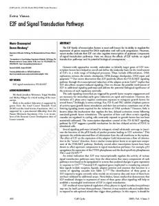
Signaling model network

Legend: Binding (complex) Activation (phosph.) Deactivation (phosph.) Chemical processing

7

Released from mitochondrion

8 4

FasL DAXX ASK-1

DAXX

FADD

6

FasL FADD2

Neurotrophin NGF

BDNF

10

11

1

FasL FADD2 FLIP

12

67

FLIP

99

70

17

PDK2

SDK1

FOXO

69 PI3K

65

71

20

55

100

GAB-1

18 p53

Akt

PTEN

22

Apaf-1 BCL-XLfree

Bax

Apaf-1

Procaspase-8

Mitochodrion

24

23

16

BIM

97

BCL-2

19

BAD BCL-XLfree

PIP3

66

13 FasL FADD2 (Procaspase-8)2

FasL FADD2 Procaspase-8 FLIP

15

SHC

Fas_Ligand

FasL FADD2 Procaspase-8

14 TRK Neurotrophin SHC GRB-2 GAB-1 PI3K SOS

GRB-2

Fas

5

9

68

64

2

Fas L FasL FADD

61

63 TRK

3

FasL FasL

Cytochrome-c

98

SOS

BAD

74 77

RAS

Akt PIP3

RAF

78 MEK1/2

75 P75ntr

Bax BCL-XL free

SGK

56

72

27

JNK

CDC42/ RAC

83

84

NF-kB

33

54 86

53

35

51 MKK4/7

ASK-1

c-jun

pRb

82

85

Ceramide

MEKK1

87

ERK1 GSK3

STEP

RSK

103

89

57

58

90

96

PLC-gamma

EGFR EGF SHC GRB-2 SOS

Apaf-1 Cytochrome-c Procaspase-9 ARC

38

zVad-fmk Caspase-8

39 Caspase 9 zVad-fmk Caspase-9

41

Caspase-9 Exec ProCaspase

48 IAP

Diablo IAP

49

46

47 Exec Caspase

92 50

94 EGF

44

Exec ProCaspase

PIP2 DAG

42

Diablo

91

93 PKC

Caspase-8

40

43

88 PAK1

NCK

37 Apaf-1 Cytochrome-c Procaspase-9

Apaf-1 Cytochrome-c (Procaspase-9)2

Forkhead

102

p19ARF

Apaf-1 Cytochrome-c ARC

52

59 MKP-1

31

32 36

81

CDK4/6

Apaf-1 Cytochrome-c

ARC

80

P75ntr Neurotrophin

30

zVad-fmk

MEKK

76

28

BCL-XL free

29

M3/6

79

Procaspase-9

26

CREB

101

ERK2

25

Caspase-8 Exec ProCaspase

45

Exec Caspase IAP

95 EGFR

Figure 1of a model signaling network Scheme Scheme of a model signaling network. Scheme of the signaling network used to demonstrate the validity of the parameter estimate method. The network consists of a series of proteins (the nodes) linked by different types of unary, binary or multiple molecular interactions (shown as the edges of the network). The role of the mitochondrion (in purple) is taken into account. Binding protein-protein interactions are shown by green edges between the nodes, activation and deactivation interactions are in blue and red, respectively, chemical transformations are shown by purple dotted lines, while the release of proteins from the mitochondria in shown in solid purple lines. The signaling process can be activated by the binding of ligands (in grey) to receptors. Every compound is identified by a name and a numerical code. N in the number of nodes, NPi,j is the number of different interactions involving the nodes i and j, NCi,j,r is the number of components when i is a protein in complex with protein j and the K i..., j represent the different rate constants. The r index accounts for different interactions between nodes i and j, when existing. The zero-th order terms Ω0i and Φ0i include the protein synthesis and the release from the mitochondria processes, the linear terms include the protein degradation, chemical autoprocessing and protein complex dissociation; the quadratic terms take into account the activation and de-activation of protein Pi, the polinomial terms describe the protein associa-

tion into larger complexes. No mass conservation constraint has been imposed to the system. In our approximation we considered both the topology of the protein interaction map and the kinetic parameters as constant in time, i.e. each protein keeps the same neighbours during the time evolution of the system and interacts with them with constant strength. We decided to completely assign the connectivity matrix of the network on the basis of the existing experimental data. On the other hand, the kinetic parameters were largely unknown on the basis on the same information sources: as a consequence, in this application, the object of the "inverse problem" are the unknown model's constants. The

Page 6 of 19 (page number not for citation purposes)

BMC Neuroscience 2006, 7(Suppl 1):S6

"inverse problem" has been implemented with the following scheme:

better and better approximation of the optimal problem's solution.

1. eqs.(5–6) are solved and the time course of variables Pi and xi (i = l...N) are calculated for a given set of model's parameters

The " inverse problem" we have attempted to solve starts from the description of a signalling network in terms of biochemical interacting species and reaction's constants. After a mining procedure to discover the value of the known reaction's constants, the system of eqs. (5–6) can be solved, by setting, for the unknown reaction's constants, an initial gauge of values. The solution of eqs.(5– 6), in terms of functions describing the predicted time course of each of the system's variables (i.e. the concentration of all the biochemical species of the network), is thus strictly related to the intial set of reaction's constants. If one defines, as individual of the GA, the complete set of reaction's constants (the l known constants and the N - l unknown constants), its ability to produce an optimal solution to the problem can be measured by evaluating the " distance" between the predicted time-course (fpred) of some variables and that effectively measured by an experimental test of the same variables on that network (fexp). Formally, a distance between the two functions representing the j-th variable can be defined as follows:

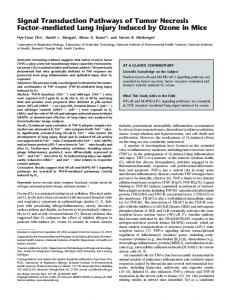
2. the predicted time course of certain quantities is compared with the corresponding experimental data and a specific "distance" between time-courses evaluated 3. procedure is iterated up to minimizing that distance Although, at least in principle, the strategy is simple, in practice the space of parameters to be estimated is very large, thus the strategy of points (1–3) above must rely on the availability of an efficient optimization algorithm. We have resorted to choose Genetic Algorithms (GA) for a number of reasons which will be highlighted in the following section.

GA: generality, numerical and computational implementation The genetic algorithm (GA) is a programming technique that mimics biological evolution as a problem-solving strategy. Given a specific problem, the input to the GA is a set (called a "population") of potential solutions (called "individuals") to that problem. Each individual contains a "genome" able to provide a sub-obtimal solution to the problem. This ability could be quantified if a specific fitness function is defined, able to quantify how much an individual, by means of its genome, is fit for the solution of the optimization problem (i.e. to measure the "distance" between the sub-optimal and the optimal solution). The purpose of the GA is to produce successive population of individuals which are generated with the aim of increasing, as much as possible, the fitness of their individuals, i.e. their ability to solve the optimization problem by decreasing that "distance". This is done by producing successive populations of individuals by using the same procedures of the natural selection: mating and mutation. In the GA workflow, given an initial population of individuals, these are evaluated and classified according to their fitness. A selection rule is then defined to allow mating of couples of individuals, that mix their genomes, to form new ones (a further population) and an appropriate frequency of mutation of the genomes is defined, to introduce "new tracts" into individuals (which, in turn, would have been composed only by tracts coming from previous populations). If selection rules for mating and frequency of mutation are appropriatly chosen, the GA produces successive sets of individuals (" generations") which are progressively more and more fit to the optimization problem. In other words, individuals are

t

(

dj = ∑ fj i =1

( pred)

(exp)

(i) − f j

(i)

)

(7)

where t is the (discrete) time length of the trajectories spanned by the variables. If one has k experimentally measured variables, the overall distance between that solution and the "optimal" solution would be k

d = ∑ di i =1

(8)

Eq.(8) can be thus retained as the "fitness" function of the considered individual; one can thus measure its "distance" from the "optimal" solution. Indeed, a more general formulation of the fitness function could be given by attributing "empirical" weight factors α to each variable, as to produce a different impact on the overall d value k

d = ∑ α i di i =1

( 9)

The aim of the GA is to produce solutions which progressively reduce the value of the distance of its individuals. The scheme of producing successive "generations" of individuals can be resumed as follows: 1. start with a set of initial N individuals {Ki, i = 1, n}, each consisting of the same l known constants and by a number n - l of randomly selected guesses of the unknown constants (Fig. 2). Each value of Ki is a real number in the interval [10-5,100]. The interval was chosen on the basis of Page 7 of 19 (page number not for citation purposes)

BMC Neuroscience 2006, 7(Suppl 1):S6

Network of interacting proteins

Architecture P2

Matrix of kinetic parameters P1

P2

…

P1

C11

C11

…

P2 … P7

C21 …

C22 …

… …

P3

P1

P7

Application of “genetic operators” to the “genomes”, the sets of unknown kinetic parameters{ Kij } P7

Next generation 5

C77

BBBBBBBBBBBBBBBBBBBBBBBBBBBBBBBBBBBBBBBBBBBBBB

Population 1 / CPU1

BBBBBBBBBBBBBBBBBBBBBBBBBBBBBBBBBBBBBBBBBBBBBB BBBBBBBBBBBBBBBBBBBBBBBBBBBBBBBBBBBBBBBBBBBBBB BBBBBBBBBBBBBBBBBBBBBBBBBBBBBBBBBBBBBBBBBBBBBB BBBBBBBBBBBBBBBBBBBBBBBBBBBBBBBBBBBBBBBBBBBBBB BBBBBBBBBBBBBBBBBBBBBBBBBBBBBBBBBBBBBBBBBBBBBB BBBBBBBBBBBBBBBBBBBBBBBBBBBBBBBBBBBBBBBBBBBBBB BBBBBBBBBBBBBBBBBBBBBBBBBBBBBBBBBBBBBBBBBBBBBB

cross-over

BBBBBBBBBBBBBBBBBBBBBBBBBBBBBBBBBBBBBBBBBBBBBB

migration

P4

P6

Genome = {K1,…,Kn} P5

Population 2 / CPU2

BBBBBBBBBBBBBBBBBBBBBBBBBBBBBBBBBBBBBBBBBBBBBB BBBBBBBBBBBBBBBBBBBBBBBBBBBBBBBBBBBBBBBBBBBBBB BBBBBBBBBBBBBBBBBBBBBBBBBBBBBBBBBBBBBBBBBBBBBB BBBBBBBBBBBBBBBBBBBBBBBBBBBBBBBBBBBBBBBBBBBBBB BBBBBBBBBBBBBBBBBBBBBBBBBBBBBBBBBBBBBBBBBBBBBB BBBBBBBBBBBBBBBBBBBBBBBBBBBBBBBBBBBBBBBBBBBBBB BBBBBBBBBBBBBBBBBBBBBBBBBBBBBBBBBBBBBBBBBBBBBB

Population 3 / CPU3 BBBBBBBBBBBBBBBBBBBBBBBBBBBBBBBBBBBBBBBBBBBBBBBBBBBBB

BBBBBBBBBBBBBBBBBBBBBBBBBBBBBBBBBBBBBBBBBBBBBB BBBBBBBBBBBBBBBBBBBBBBBBBBBBBBBBBBBBBBBBBBBBBB BBBBBBBBBBBBBBBBBBBBBBBBBBBBBBBBBBBBBBBBBBBBBB BBBBBBBBBBBBBBBBBBBBBBBBBBBBBBBBBBBBBBBBBBBBBB BBBBBBBBBBBBBBBBBBBBBBBBBBBBBBBBBBBBBBBBBBBBBB BBBBBBBBBBBBBBBBBBBBBBBBBBBBBBBBBBBBBBBBBBBBBB BBBBBBBBBBBBBBBBBBBBBBBBBBBBBBBBBBBBBBBBBBBBBB

4: insufficient fitness, iterate

1

Calcultation of the Fitness Function

Simulated kinetics of protein concentrations

Fitness evolution of the best individual

10

experimental simulated

12 11 10

3

activity

9 8 fitness

2 1

7 6 5 4 3 2

0.0001

# generations

0 1 time

Good fitness, GA saturates: end procedure Reverse engineering results Set of network model parameters which can best reproduce the experimental kinetic data

Figure 2algoritm scheme Genetic Genetic algoritm scheme. Flow chart of the estimate procedure using the genetic algorithm (GA). Every unknown model parameter is called a " gene", while the whole set of parameters to be estimated is defined as the " genome". Every genome is contained within an " individual", the computational entity able to " evolve". An ensemble of genomes corresponds to a "population". The GA procedure begins with an initial random guess of the parameters values used to run a simulation of the model network. This first step is iterated for all the individuals belonging to different populations. For each individual, the simulated time course of the concentrations for specific proteins are compared with the experimental measures and the distances between the functions are calculated. Every individual is thus related to a fitness index, measuring the degree of compatibility of the genome with the experimental constraints. A small number of individuals are selected based on their fitness but also on probabilistic rules: they will have the genomes randomly mutated by genetic operators, giving birth to a new offspring that enters the next generation. At each round the plot describing the evolution of the best fitness computed until then is updated: when it clearly saturates the algorithm stops and the genome corresponding to that fitness is the solution of the algorithm.

a reasonable number of kinetic values of protein-protein interactions published in the literature 2. for each individual, evaluate the distance d of eq.(8) 3. select, according to some defined rule, the individuals to be mated to form the new generation of individuals.

4. perform the mating procedure as follows: given two different individuals {KA(i)} and {KB(i)}, we randomly select the index m (l 2: the range becomes α ∈ [-5 * (NC - 2), 0]. The Fitness Function F() is here defined, for each individual, as the inverse of the squared Euclidean distance between the experimental time course of the concentration of the activated fraction of ERK-1, c-Raf, MEK, PKCiota proteins (see above) and the simulated time course for the same species, obtained using the genome {K1,...,Kn} of the individual (Fig. 2, step 2) as parameters set; this distance is evaluated across the whole time interval (60 minutes), with a sampling time of 2 minutes: ⎡ pnp t Nt ⎤ F(K1 ,..., K n ) = ⎢ ∑ ∑ ( X pexp (t ) − xpsim (t ))2 ⎥ ⎢ p= p1 t =t ⎥ 1 ⎣ ⎦

Si max{Si , i ∈ population}

( 13 )

where 10-4