parameter estimation for weibull distribution with right censored data ...

Article citation info: Ferreira LA, Silva JL. Parameter estimation for Weibull distribution with right censored data using EM algorithm. Eksploatacja i Niezawodnosc – Maintenance and Reliability 2017; 19 (2): 310–315, http://dx.doi.org/10.17531/ein.2017.2.20.

Luís Andrade Ferreira José Luís Silva

Parameter estimation for Weibull distribution with right censored data using EM algorithm Zastosowanie algorytmu maksymalizacji wartości oczekiwanej do estymacji parametrów rozkładu Weibulla w przypadku danych obciętych prawostronnie The maximum-likelihood estimation (MLE) is a method of estimating the parameters of a statistical model for given data. This method allows us to estimate the unknown parameters of a statistical model. These parameters are obtained by maximizing the likelihood function of the model in question. In many practical situations the likelihood function is associated with complex models and the likelihood equation has no explicit analytical solution, it is only possible to have its resolution through numerical methods. The estimation of the parameters of the Weibull distribution by maximum-likelihood method based on information from a historical record with right censored data shows this difficulty. The solution presented in this article entails using the ExpectationMaximization (EM) algorithm. Actual data from the historical record of 5 centrifugal pumps failures of a petrochemical company were analyzed for application of the methodology. Keywords: EM algorithm, parameter estimation, maximum likelihood estimates, reliability. Metoda największej wiarygodności (MLE) służy do estymacji parametrów modelu statystycznego dla zadanych danych. Metoda ta pozwala na estymację nieznanych parametrów modelu statystycznego. Parametry te otrzymuje się poprzez maksymalizację funkcji wiarygodności rozważanego modelu. Często w praktyce metoda ta może jednak nastręczać trudności związane z wielomodalnością funkcji wiarygodności oraz niemożnością uzyskania jawnych analitycznych rozwiązań równań wiarygodności. Równania takie można jedynie rozwiązywać za pomocą metod numerycznych. Trudności te dobrze ilustruje estymacja parametrów rozkładu Weibulla z wykorzystaniem metody największej wiarygodności wykonywana w oparciu o prawostronnie cenzurowane dane z eksploatacji. Rozwiązanie przedstawione w niniejszej pracy opiera się na zastosowaniu algorytmu maksymalizacji wartości oczekiwanej (EM). Możliwości aplikacyjne proponowanej metodyki badano na przykładzie danych eksploatacyjnych uzyskanych z przedsiębiorstwa petrochemicznego, dotyczących awarii pięciu pomp odśrodkowych. Słowa kluczowe: algorytm EM, estymacja parametrów, estymator największej wiarygodności, niezawodność.

1. Introduction The estimation process is supported by a number of statistical techniques, methods and procedures for analyzing the data on the variable of interest that may be the time that elapses from the welldefined initial instant, for example, installation of equipment, until the occurrence of a specific event, such as the failure of the equipment or component under consideration. The process aims to estimate the distribution parameters for modeling the system under review. The parameters are the distribution characteristics that show the behavior of a given population and therefore fixed for a specific system. Thus, the estimation of system parameters is obtained from the data collected from the population. System data analysis can be obtained from various possible sources, namely, laboratory tests or a recording of occurrences along its use (historical record). The parametric analysis assumes that the data fits a specific distribution, such as the Weibull distribution. The Weibull distribution has a wide application in various fields. These applications include its use to model the distribution phenomena of fatigue and the life of many devices, such as bearings, shaft and motor [1, 14, 20].

310

The popularity of the distribution of Weibull due to its great flexibility, i.e., as it can describe functions with failure intensity constant, increasing and decreasing, for different values of the shape parameter. Since the distribution of Weibull became widely recognized, various methods have been proposed to estimate its parameters [2,17,19]. However, the maximum-likelihood estimation method is currently one of the most used methods of estimation, for its versatility and provides reliable results [10]. The maximum-likelihood estimation method allows us to estimate the unknown parameters of a statistical model. These parameters are obtained by maximizing the likelihood function of the model in question [4].

2. Types of data With the information from a historical record of data is possible to obtain indicators to estimate and understand the behavior of the equipment with respect to failures. Therefore, using appropriate methodologies, it will be possible to set the proper maintenance policies to any equipment and their components.

Eksploatacja i N iezawodnosc – Maintenance and Reliability Vol.19, No. 2, 2017

S cience and Technology The data is considered complete when it is known the exact time of each system failure. In many cases the data contain uncertainties, i.e., it is not known the exact moment when the failure occurred. The data containing such uncertainty as to when the event occurred are regarded as incomplete or partial. Incomplete data can be classified into censored or truncated [8, 13]. Incomplete data give only part of the information about the failure time of the units under review. However, this information should not be ignored or treated as failure. In the absence of such data, it would not be possible to make good estimation parameters and thus make a proper analysis. One of the most common types of censored data, which may arise in real cases, is Type-1 right censored data [9]. For Type-1 right censored data, all units of a system are observed up to the date of completion of the study. For this censorship scheme the time each unit is under observation is fixed, while the number of units that fail (uncensored observations) is random. If T is a random variable representing the failure time and Cd another random variable independent of T which corresponds to the end of the registration information (observation time). It is said that the time to failure is right censored when one does not know its exact value, only that its value is greater than Cd, with regard to item i (i = 1, 2, ..., n). Therefore:

1 if Ti ≤ Cdi ti = min (Ti , Cdi ) and δ i =  0 if Ti > Cdi

 1, for uncensored data δi =   0, for censored data





(2)

In the right censored data the failure time of the units with censored data it is just known to be greater than the operating time of the conclusion of the registration information. These right censored data are further classified into Type-1 if the recording of information is interrupted at a predetermined time and Type-2 censure if registration is completed when a predetermined number of failures occur [12].

L (θ1,θ 2 ,…,θ k ) =

∏ f ( xi |θ1, θ 2 ,…,θk ) ∏ 1 − F ( xi |θ1,θ 2 ,…,θ k )

δ i =1

δi =0

(3)

Where (x1, x2, ..., xn) is a sample of n independent observations of the random variable X and θ = (θ1, θ2, ..., θk) is the vector of unknown distribution parameters.

1−δ i

  t  β  i exp  −     η  

(4)

β

n n n t   (5) ln L (η , β ) = l (η , β ) = ∑ ( nδ i ln β − nβδ ilnη ) + ( β − 1) ∑ (δ i ln ti ) − ∑  i  � � � (5) i =1  η  i =1 i =1

As the maximum-likelihood equations in many cases have no analytical solution to determine their solutions, it is needed to use numerical optimization methods. Among the possible numerical solutions, in this paper the Expectation-Maximization (EM) algorithm was selected [3, 5, 15].

3.1. The Expectation-Maximization algorithm The EM algorithm is an iterative process that can be used to calculate the maximum likelihood estimators in cases with incomplete data. Let X be the set of complete data with the probability density function fc (x, θ) and Y the observed data. The corresponding loglikelihood function to the full sample is represented by: ln Lc ( x,θ ) = lc ( x,θ )



(6)

Each iteration of the EM algorithm involves two steps: step E (expectation) and step M (maximization), defined by [15],

)

(

Step E: To calculate Q θ ,θ ( k ) , where:



3. The maximum-likelihood estimation method As we have seen, in the particular case of the right censored data classified as Type-1 censorship, the recording of information is interrupted at a predetermined time Cd > 0, such that ti is observed to occur before Cd, otherwise, one only knows that the failure time is greater than the observation time. Let ti = t1, t2, ..., tn, n independent observations, where r records are failure times and (n - r) are censured information. Let the probability density function, f(x, θ) and the cumulative probability function F(x, θ), with the distribution parameters denoted by θ, the likelihood function for right censored data Type-1 is given by [18]:

δi

 β  t  β −1   t  β    L (η , β ) = ∏   i  exp  −  i      η   η η i =1       n

In many situations it is easier to achieve the maximization of the log of the likelihood function and, since the logarithm function is a monotonically increasing function, is equivalent to maximizing the likelihood function or the log-likelihood function. By applying logarithm to eq. 4, it becomes:

(1)

The δi variable (censorship indicator) indicates whether Ti is censored or not. The obtained data can be represented by the pair (ti, δi) i.e. ti the failure time or censored time and δi the variable that indicates whether it concerns a failure or censorship, that is, (2):

For the Weibull distribution with scale parameter η and shape parameter β, the likelihood function for the right censored data Type-1 is given by:

)

(

k k −1 Q θ ,θ ( ) = E ( k ) lc ( x,θ ) y, δ ,θ ( )    θ

Step M: To find θ (



k +1)

(

(7)

)

that maximizes Q θ ,θ ( k ) , that is:

( ) Q (θ ( ) ,θ ( ) ) ≥ Q (θ ,θ ( ) ) θ(

k +1)

k = arg max Q θ ,θ ( )

k +1

k

k

(8)

The procedure is performed until the difference between the iteration k and iteration k+1:

(

 = L θ(

k +1)

) − L (θ ( ) ) k

(9)

decrease to an acceptable value, with  > 0 In Step E the algorithm calculates the conditional expected value of the logarithm of the likelihood function for complete data given the observed sample and step M calculates its maximum.

Eksploatacja i N iezawodnosc – Maintenance and Reliability Vol.19, No. 2, 2017

311

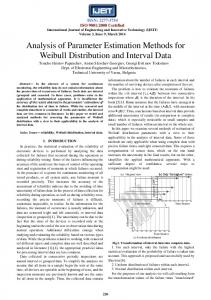
S cience and Technology This algorithm requires an initial solution for the values of the distribution parameters, designated by θ(0). The selection of this initial solution requires particular attention to the extent that the algorithm convergence speed may become extremely slow due to a poor choice. Another aspect to take into account is the maximum likelihood equation can have multiple solutions corresponding to local maxima, so the choice of the starting solution becomes important. A comparative study of various strategies in the choice of initial values can be found in Karlis and Xekalaki [11]. The results obtained by these authors demonstrate the importance of the choice of initial values, to have a reasonable convergence speed. The figure 1 illustrates the EM algorithm procedure.

3.2. EM algorithm with right censored data The observed data consists of (Yi, δi), with Yi = min (Ti, Cdi), where Cdi corresponds to the observation times, δi = 1 (Ti ≤ Cdi), corresponds to the non-censored data and δi = 0 (Ti > Cdi), to the censored data. In the step E of the algorithm it is required the calculation of the conditional expected value of the log-likelihood for complete data, given the observed sample. In this case the log-likelihood function to complete data is given by equation (10), for n data collected: β

n t  n ln L (η , β ) = l (η , β ) = n ln β − nβ lnη + ( β − 1) ∑ ( ln ti ) − ∑  i  (10) i =1  η  i =1

The θ = (η, β) are the distribution parameters, δ = (δ1, δ2, ..., δn) is the vector indicator of censorship and y = (y1, y2, ..., yn) is the vector of observed data. We have from equation (7):

)

(

n

n

i =1

i =1

k Q θ ,θ ( ) = nln �� β − nβ lnη + ( β − 1) ∑ Ai − ∑Bi



(11)

Where: Ai = E ( k ) ln ti yiδ  = δ i ln yi + (1 − δ i ) E ( k ) ln ti ti > yi  θ θ



(12)

Bi = E ( k ) tiβ yiδ  = δ i yiβ + (1 − δ i ) E ( k ) tiβ ti > yi  (13)     θ θ



For the conditional expected value is first necessary to determine the expression of the corresponding conditional probability density function, f(y|y’) (y|y’). For this case is given by [16]: Fig. 1. EM algorithm procedure

The EM algorithm has several advantages which stand out relative to other iterative algorithms: –– The EM algorithm converges in a large variety of conditions, that is, from an arbitrary data, θ(0) the algorithm usually finds a local maximum, except for a poor choice of initial solution θ(0) or in the wrong formulation of the likelihood function. –– The required analytical work is simpler than with other methods, since only it is necessary to maximize the conditional expected value of the log-likelihood for complete data. –– The EM algorithm is relatively easy to program and implement. –– During the iterations it is possible to control the convergence and programming errors However it also has some disadvantages: –– The EM algorithm can converge slowly, even in some apparently simple problems and on issues where there is a lot of incomplete information. –– The EM algorithm does not have an integrated process for producing an estimate of the covariance matrix of the estimated parameters. But this disadvantage can be overcome by using appropriate methodology. –– The EM algorithm does not guarantee convergence to the global maximum when there are multiple maximum sites. The obtained estimate depends on the initial solution

f ( ti |yi ) =



β  ti    η η 

β −1

β

 y  t  exp  i  −  i   η  η  

β

 ,� � ti > yi  

(14)

So,  y  1 E ( k ) ln ti t > yi  = ln yi + exp  i  k) (  η (k )  θ β  



E ( k ) tiβ t > yi  = yiβ   θ

(k )

k β( )

k  β( )    yi    “ 0,    (15)  η (k )       

( )

k + η( )

k β( )



(16)

Where: ∞

Γ ( p, x ) = ∫u p −1e −u du , is the upper incomplete gamma function. x

Introducing equations (15) and (16) in equations (12) and (13): k k  β( )  β ( )   y   y      1 Ai = δ i ln yi + (1 − δ i ) ln yi + exp  i  “ 0,  i   k) k)  k)  ( ( (   β   η   η     

(17)

312

Eksploatacja i N iezawodnosc – Maintenance and Reliability Vol.19, No. 2, 2017

S cience and Technology  (k ) k Bi = δ i yiβ + (1 − δ i )  yiβ + η ( )  

( )



k β( ) 

  

(18)

Thus, the expression referring to step E of the algorithm EM, Q(θ,  θ(k)) with censored data to the right is given by the following equation:   1 k … Q θ ,θ ( ) = n ln β − nβ lnη + ( β − 1) ∑ δ i ln yi + (1 − δ i ) ln yi + k  β( ) i =1   k k β( )  β ( )   k  (k ) β ( )   y    yi    1 n  β k i     − β ∑ δ i yi + (1 − δ i )  yiβ + η ( ) exp  Γ 0,      η (k )   η (k )    η i =1              

)

(

n

( )

(19) As mentioned above, the step M is intended to find the solution θ (k+1) which maximize Q(θ, θ (k)). In order to get the points that maximize the function it is necessary to solve the partial derivatives of the above equation and equal them to zero, as shown in the following equations:

(

k ∂Q θ ,θ ( )

∂η

) = − nβ + η

  (k )  β  yiβ + η ( k ) δ δ + − 1 y ( )  ∑ i i i  η β +1 i =1   

( )

n

β

k β ( )  

  

(20)

(

k ∂Q θ ,θ ( )

∂β

) = n − n ln η + ∑ δ ln y + (1 − δ ) ln y + n

β

i

i =1 

i

i



 

i

 y  1 exp  i  k) (  η (k )  β  

k  β ( )     (k )   n  lnη  β   yi  k β  Γ 0,  + η( )   + ∑  β δ i yi + (1 − δ i )  yi  η (k )       i =1  η      

( )

k β( )

…

k β ( )  

 1 − δ i yiβ ln yi   η β  

(21) Thus, the solution for the estimation of the distribution parameters η is given by the following equation: 1

k   β ( )  β 1 n   y   β (k )    β k) ( β i   η = ∑ δ i yi + (1 − δ i )  yi + η exp   .η  η (k )  i =1         

(22)

With equation (22) for η parameter, it is possible to calculate the β parameter of the distribution. The second derivative must be negative to ensure that the results obtained correspond to a maximum point. The second derivative equations are as follows:

(

k ∂ 2Q θ , θ ( )

∂η 2

(

k ∂ Q θ ,θ ( ) 2

∂β

2

) = nβ − β ( β + 1) ∑ δ y n

η β +2

η2

) = − n − (lnη ) β

2

η

β

+

i =1  

β i i

 (k ) k + (1 − δ i )  yiβ + η ( )  

( )

k β ( )  

  

(23) 2 n

 



∑ δ i yiβ + (1 − δ i )  yiβ

i =1  



2 lnη

∑ (δ i yiβ ln yi ) −

η

β

n

i =1

(k )

1

η

β

( )

k + η( ) n

k β ( )  

 …  

∑ δ i yiβ ( ln yi )

i =1

2

 �

(24)

(

k ∂ 2Q θ , θ ( )

∂η∂β

) = ∂ Q (θ ,θ ( ) ) = − n + 1 − β lnη ∑{δ y

 (k )  yiβ + η ( k )  

( )

k

2

n

∂β∂η

η

k β ( )  

η β +1

β n  + ∑ δ i yiβ ln yi β   η +1 i =1 

(

i =1

β i i

+ (1 − δ i )…

) (25)

With this analysis it is possible to calculate the Weibull distribution parameters β and η, through the knowledge of the maximum values of function Q.

4. Case study The case study concerns the history of five centrifugal pumps failures of a petrochemical company, used to pump oil with similar density for the period 2006 to 2013. From the collected data it can be seen that one of the pumps components is responsible for an important number of failures. It is the mechanical seal which represents approximately 45% of the total number of failures. Thus, based on the assessment of these results, it justifies the need of further study on this component. For the purposes of this study, we select only the data related to failures due to excessive leakage of fluid to the outside of the pumps. The reason for this consideration is due to the significant number of failures and to restrict the study for just one failure mode. The possible failures between inspections are treated as complete data, as the centrifugal pumps in question are visually inspected by the user of the equipment at least every 8 hours. So, it was not considered the possible mistake between two inspections compared to the total time of the observation and it was assumed that the exact moment of failure was well known. The last record in each pump does not correspond to a fault but at the end of the test, since the pumps continued in operation. Thus the last recording time of each pump was considered as right censored data. For the estimated values of the Weibull distribution parameters by the maximum-likelihood method it was used the EM algorithm for right censored data as described in section 3.2. For the algorithm implementation process it was used the statistical program R. The autors used a manually written code in R software and also used some packages like for exemple, maxNR, boot and mass. The initial solution θ(0) was attributed by the result obtained by the least squares method. The iterative process stopped when the difference between the iteration k and iteration k+1, given by equation (9), was less than 0,1. The following Table 1 shows the expected value for βˆ and ηˆ for each of the mechanical seals applying the maximum-likelihood method with the EM algorithm, as described in this paper. The respective confidence intervals are also presented. Table 1. Expected value of βˆ and ηˆ (days) for each of the mechanical seals obtained with the maximum-likelihood method (EM) and respective confidence interval by the bootstrap-T method Mechanical seals

βˆ

1

6,12

9,21

14,09

365,51

3

10,85

13,92

17,19

385,03

5

3,96

7,56

2

4

2,01

4,93

5,04

8,17

10,12

12,98

12,51

Eksploatacja i N iezawodnosc – Maintenance and Reliability Vol.19, No. 2, 2017

301,49

352,85

335,62

ηˆ (days) 392,96

425,53

403,68

423,21

345,31

381,44

368,37

392,67

416,05

406,99

313

S cience and Technology Because the sample of data is small, it was used the bootstrap-t method in determining the confidence intervals with a confidence level of 95% [6, 7]. The bootstrap-t method allows the calculation of the confidence interval of the parameters of interest in particular in the case where the sample is small (n 1. The values of the scale parameter η vary between 345.31 and 403.68 days of operation. With the information obtained by the bootstrap method, it is possible to represent the confidence interval around the probability density function of the estimated Weibull distribution, as shown in Figure 2 to seal 1.

Table 2. Expected value of βˆ and ηˆ (days) for each of the mechanical seals obtained with the least squares method Mechanical seals

βˆ

1

8,76

3

12,54

5

6,55

2 4

4,26 7,68

ηˆ (days) 388,72 338,17 415,15 386,71 363,42

The estimation of the unknown parameters of the Weibull distribution was also obtained, in the same system, with the least squares method, to compare with the results obtained by the EM algorithm. In Rinne is indicated how to obtain the estimates of the unknown parameters using least squares method. The following Table 2 shows the expected value for βˆ and ηˆ for each of the mechanical seals applying the least squares method. The shape parameter, β, is higher by maximum likelihood method (EM algorithm) than the least squares method and in both is higher than 1. For the scale parameter, η, the values obtained by the two methods are similar.

5. Conclusion The prediction of failures of equipment for a given time horizon can only be considered in probabilistic terms, because there is always uncertainty about the time they will happen. Thus, this work has focused on the presentation of statistical techniques inherent to an estimation process of the parameters of a theoretical probabilistic model that best fits the observed data. Also, it showed the importance of the record of occurrences of failures during the use of equipment (historical record). This information is essential for monitoring a system, and also for the correct performance of the maintenance activities. However, some data may contain uncertainty regarding the time of occurrence of the failures and thus are regarded as incomplete or partial. Due to the complexity of the analyzed data, in particular in the presence of right censored data, it was found that the equation from the maximum-likelihood method showed no analytical solution. So the solution presented in this work was using the EM algorithm. In this work it was possible to validate the applicability of the EM algorithm to determine the solutions of the equation that is derived from the maximum-likelihood method in the presence of incomplete data. Acknowledgement The research work partially financed by FCT (portuguese Foundation for Science and Technology.

Fig. 2. Confidence interval around the probability density function of the estimated Weibull distribution by the bootstrap method, seal 1

References 1. 2. 3. 4.

Abernethy R B. The New Weibull handbook. Florida: Robert B. Abernethy, 2006. Akram M, Hayat A. Comparison of estimators of the Weibull distribution. Journal of Statistical Theory and Practice 2014; 8(2): 238-259, https://doi.org/10.1080/15598608.2014.847771. Balakrishnan N, Mitra D. Left truncated and right censored Weibull data and likelihood inference with an illustration. Computational Statistics and Data Analysis 2012; 56: 4011-4025, https://doi.org/10.1016/j.csda.2012.05.004. Balakrishnan N, Kundu D, Ng H K T. Point and interval estimation for a simple step-stress model with type-II censoring. Journal of Quality Technology 2007; 39: 35-47.

314

Eksploatacja i N iezawodnosc – Maintenance and Reliability Vol.19, No. 2, 2017

S cience and Technology 5. 6. 7. 8. 9. 10. 12. 13. 14. 15. 16. 17. 18. 19. 20. 21.

Chambers R L, Steel D G, Wang S, Welsh A H. Maximum likelihood estimation for sample surveys. Boca Raton, Florida: Chapman and Hall/ CRC Press, 2012. Dempster A P, Laird N M, Rubin D B. Maximum likelihood from incomplete data via the EM algorithm. Journal of the Royal Statistical Society 1977; 39(1): 1-38. Efron B, Tibshirani R J. An introduction to the bootstrap. London: Chapman & Hall, 1993, https://doi.org/10.1007/978-1-4899-4541-9. Fang L Y, Arasan J, Midi H, Bakar M R A. Jackknife and bootstrap inferential procedures for censored survival data. AIP Conference Proceedings 2015; 1682: 1-6, https://doi.org/10.1063/1.4934631. Gijbels I. Censored data. Wires Computational Statistics 2010; 2: 178 - 188, https://doi.org/10.1002/wics.80. Guure C B, Ibrahim N A. Methods for estimating the 2-parameter Weibull distribution with type-I censored data. Journal of Applied Sciences, Engineering and Technology 2013; 5(3): 689-694. Karlis D, Xekalaki E. Choosing initial values for the EM algorithm for finite mixtures. Computational Statistics and Data Analysis 2003; 41: 577-590, https://doi.org/10.1016/S0167-9473(02)00177-9. Kinaci I, Akdogan Y, Kus C, Ng H K T. Statistical inference for Weibull distribution based on a modified progressive type-II censoring scheme. Sri Lankan Journal of Applied Statistics 2014; 1: 95-116, https://doi.org/10.4038/sljastats.v5i4.7786. Lawless J F. Statistical models and methods for lifetime data. New Jersey: John Wiley & Sons, 2003. McCool J I. Using the Weibull distribution, reliability, modeling and inference. New York: John Wiley & Sons, 2012, https://doi. org/10.1002/9781118351994. McLachlan G J, Krishnan T. The EM algorithm and extensions. New Jersey: John Wiley & Sons, 2008, https://doi. org/10.1002/9780470191613. Ng H K T, Chan P S, Balakrishnan N. Estimation of parameters from progressively censored data using EM Algorithm. Computational Statistics and Data Analysis 2002; 39: 371-386, https://doi.org/10.1016/S0167-9473(01)00091-3. Procaccia H, Ferton É, Procaccia M. Fiabilité et maintenance des matériels industriels réparables et non réparables. Paris: Ed. Tec & Doc, 2011. Rinne H. The Weibull distribution - A handbook. Florida: CRC Press, 2009. Teimouri M, Hoseini S M, Nadarajah S. Comparison of estimation methods for the Weibull distribution. Statistics: Journal of Theoretical and Applied Statistics 2013; 47(1): 93-109, https://doi.org/10.1080/02331888.2011.559657. Tobias P A, Trindade D C. Applied reliability. Florida: Chapman & Hall/CRC Press, 2011.

Luís Andrade Ferreira FEUP - Faculdade de Engenharia da Universidade do Porto Department of Mechanical Engineering Rua Dr. Roberto Frias, 4200-465, Porto, Portugal José Luís Silva ESTV – Escola Superior Tecnologia de Viseu Department of Mechanical Engineering and Industrial Management Campus Politécnico, 3504-510, Viseu, Portugal E-mail: [email protected], [email protected]

Eksploatacja i N iezawodnosc – Maintenance and Reliability Vol.19, No. 2, 2017

315