Parameter-Free Deterministic Global Search with

Parameter-Free Deterministic Global Search with Simplified Central Force Optimization Richard A. Formato Registered Patent Attorney & Consulting Engineer P.O. Box 1714, Harwich, MA 02645, USA [email protected]

Abstract. This note describes a simplified parameter-free implementation of Central Force Optimization for use in deterministic multidimensional search and optimization. The user supplies only the objective function to be maximized, nothing more. The algorithm’s performance is tested against a widely used suite of twenty three benchmark functions and compared to other state-ofthe-art algorithms. CFO performs very well. Keywords: Central Force Optimization, CFO, Deterministic Algorithm, Multidimensional Search and Optimization, Parameter-Free Optimization, Gravitational Kinematics Metaphor, Metaheuristic.

1 Introduction Central Force Optimization (CFO) is a deterministic Nature-inspired metaheuristic for an evolutionary algorithm (EA) that performs multidimensional global search and optimization [1-13]. This note presents a simplified parameter-free CFO implementation that requires only one user-specified input: the objective function to be maximized. The algorithm performs quite well across a wide range of functions. A major frustration with many EAs is the plethora of setup parameters. For example, the three Ant Colony Optimization algorithms described in [14] (AS, MAX-MIN, ACS) require the user to specify nine parameters The generalized Particle Swarm Optimization algorithm in [15] requires the user to specify a population size and six “suitable bounded coefficients”. This frustration is compounded by the facts that (a) there usually is no methodology for picking “good” values; (b) the “right” parameters are often problem-specific; (c) the solutions often are sensitive to small changes; and (d) run upon run, exactly the same parameters never yield the same results because the algorithm is inherently stochastic. CFO is quite different. It is based on Newton’s laws of motion and gravity for real masses moving through the real Universe; and just as these laws are mathematically precise, so too is CFO. It is completely deterministic at every step, with successive runs employing the same setup parameters yielding precisely the same results. Its inherent determinism distinguishes CFO from all the stochastic EAs that fail completely if randomness is removed. Moreover, CFO’s metaphor of gravitational kinematics appears to be more than a simple analogy. While many metaheuristics are D.-S. Huang et al. (Eds.): ICIC 2010, LNCS 6215, pp. 309–318, 2010. © Springer-Verlag Berlin Heidelberg 2010

310

R.A. Formato

inspired by natural processes, ant foraging or fish swarming, for example, the resulting algorithm is not (necessarily) an accurate mathematical model of the actual process. Rather, it truly is a metaphor. By contrast, CFO and real gravity appear to be much more closely related. Indeed, CFO’s “metaphor” actually may be reality, because its “probes” often exhibit behavior that is strikingly similar to that of gravitationally trapped near earth objects (NEOs). If so, the panoply of mathematical tools and techniques available in celestial mechanics may be applicable to CFO directly or with modification or extension (see [1,7-9]). CFO may be interpreted in different ways depending upon the underlying model (vector force field, gravitational potential, kinetic or total energy) [3,13]. These observations, although peripheral to the theme of this note, provide additional context for the CFO metaheuristic. There are, of course, other gravity-inspired metaheuristics, notably Space Gravitational Optimization [16]; Integrated Radiation Optimization [17]; and Gravitational Search Algorithm [18, 19]. But each one is inherently stochastic. Their basic equations contain true random variables whose values must be computed from a probability distribution and consequently are unknowable in advance. CFO, by contrast, is completely deterministic. Even arbitrarily assigned variables (for example, the “repositioning factor” discussed below), are known with absolute precision. At no point in a CFO run is any value computed probabilistically, which is a major departure from how almost all other Nature-inspired metaheuristics function.

2 CFO Algorithm Pseudocode for the parameter-free CFO implementation appears in Fig. 1. Simplification of the algorithm is accomplished by hardwiring all of CFO’s basic parameters, which results in simplified equations of motion as described below. CFO searches for the global maxima of an objective function

f ( x1 , x2 ,..., xN d ) defined on the

Ω : ximin ≤ xi ≤ ximax , 1 ≤ i ≤ N d . The xi are G G decision variables, and i the coordinate number. The value of f (x ) at point x in G Ω is its fitness. f (x ) ’s topology or “landscape” in the N d -dimensional hyper-

N d -dimensional

decision space

space is unknown, that is, there is no a priori information about the objective function’s maxima. CFO searches Ω by flying “probes” through the space at discrete “time” steps (iterations). Each probe’s location is specified by its position vector computed from two equations of motion that analogize their real-world counterparts for material objects moving through physical space under the influence of gravity without energy dissipation. Probe

Nd G p ’s position vector at step j is R jp = ∑ xkp , j eˆk , where the xkp , j are its k =1

coordinates and

eˆk the unit vector along the xk -axis. The indices j , 0 ≤ j ≤ N t ,

and

p , 1 ≤ p ≤ N p , respectively, are the iteration number and probe number, with

Nt

and

Np

being the corresponding total numbers of time steps and probes.

Parameter-Free Deterministic Global Search with Simplified Central Force Optimization

In metaphorical “CFO space” each of the

Np

311

probes experiences an acceleration

Ω (see [1,12] for details).

created by the “gravitational pull” of “masses” in Probe p ’s acceleration at step j − 1 is given by

G G Np ( R kj−1 − R jp−1 ) Gp k p k p , a j −1 = ∑ U ( M j −1 − M j −1 ) ⋅ ( M j −1 − M j −1 ) × G k G R j −1 − R jp−1 k =1

(1)

k≠ p

which

M

p j −1

probe

is

the

first

p , j −1 1

= f (x

,x

of

p , j −1 2

CFO’s

,..., x

p , j −1 Nd

two

)

equations

of

motion.

In

(1),

is the objective function’s fitness at

p ’s location at time step j − 1 . Each of the other probes at that step (iteration)

has associated with it fitness

M kj−1 , k = 1,..., p − 1, p + 1,..., N p . U (⋅)

is the

Gk Gp ⎧1, z ≥ 0 ⎫ U ( z) = ⎨ ⎬ . If R j −1 = R j −1 , k ≠ p , then ⎩0, otherwise⎭ G Gp k p a j −1 ≡ 0 because M j −1 = M j −1 and a jp−1 is indeterminate (probes k and p have coalesced so that k cannot exert a gravitational force on p ). The acceleration G G G a jp−1 causes probe p to move from position R jp−1 at step j − 1 to position R jp at step j according to the trajectory equation G G G R jp = R jp−1 + a jp−1 , j ≥ 1 , (2) Unit Step function,

which is CFO’s second equation of motion. These simplified CFO equations result

from hardwiring CFO’s basic parameters to G = 2 , Δt = 1 , α = 1 , and β = 1 (see [1,11,12] for definitions and discussion). The “internal parameters” in Fig. 1 are not fundamental CFO parameters, but rather specific to this particular implementation. Every CFO run begins with an Initial Probe Distribution (IPD) defined by two variables: (a) the total number of probes used, placed inside

Np ;

and (b) where the probes are

Ω . The IPD used here is an orthogonal array of

Np Nd

probes per

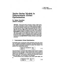
dimension deployed uniformly on “probe lines” parallel to the coordinate axes and intersecting at a point that slides along Ω ’s principal diagonal. Fig. 2 provides a two-dimensional (2D) example of this type of IPD (9 probes shown on each probe line, 2 overlapping, but any number may be used). The probe lines are parallel to the x1 and x2 axes intersecting at a point on Ω ’s principal diagonal marked by position vector

G G G G D = X min + γ ( X max − X min ) . The diagonal’s endpoints are at

312

R.A. Formato

G

Procedure CFO [ f ( x ) , N d , Ω] min init , ΔFrep , Frep , N t , Frep

Internals:

⎛ Np ⎞ , ⎜⎜ ⎟⎟ N ⎝ d ⎠ MAX

γ start , γ stop , Δγ

.

global G f max ( x ) = very large negative number, say, − 10 +4200 .

Initialize

by 2 : For N p N d = 2 to ⎛⎜ N p ⎞⎟ ⎜N ⎟ ⎝ d ⎠ MAX Total number of probes: N = N ⋅ ⎛⎜ N p ⎞⎟ p d ⎜ ⎟

(a.0) For

γ = γ start

to

γ stop

by

Δγ

⎝ Nd ⎠

:

(a.1) Re-initialize data structures for position/ acceleration vectors & fitness matrix. (a.2) Compute IPD [see text]. (a.3) Compute initial fitness matrix, M 0p ,1 ≤ p ≤ N p . (a.4) Initialize For

init . Frep = Frep

j = 0 to N t [or earlier termination – see text]: (b)

G

Compute position vectors, R jp , 1 ≤ p ≤ N p [eq.(2)].

Retrieve errant probes ( 1 ≤ p ≤ N p ): Gp G G If R j ⋅ eˆi < ximin ∴ R jp ⋅ eˆi = max{ximin + Frep ( R jp−1 ⋅ eˆi − ximin ), ximin } . G G G If R jp ⋅ eˆi > ximax ∴ R jp ⋅ eˆi = min{ximax − Frep ( ximax − R jp−1 ⋅ eˆi ), ximax } . (c)

(d)

Compute fitness matrix for current probe distribution, M jp , 1 ≤ p ≤ N p .

(e) (f)

Compute accelerations using current probe distribution and fitnesses [eq. (1)]. min Increment Frep : Frep = Frep + ΔFrep ; If Frep > 1∴ Frep = Frep ..

(g)

If j ≥ 20 and j MOD 10 = 0 ∴ (i)

Shrink Ω around

G Rbest [see text].

(ii) Retrieve errant probes [procedure Step (c)]. Next

j (h) (i)

Next

γ

Reset Ω boundaries [values before shrinking]. G G global G global G If f max ( x ) ≥ f max ( x ) ∴ f max ( x ) = f max ( x ) .

Next N p N d Fig. 1. Parameter-free CFO Pseudocode

Parameter-Free Deterministic Global Search with Simplified Central Force Optimization

313

Nd Nd G G min ˆ X min = ∑ xi ei and X max = ∑ ximax eˆi , and parameter 0 ≤ γ ≤ 1 determines i =1

i =1

where along the diagonal the probe lines intersect.

Fig. 2. Variable 2D Initial Probe Distribution

Fig. 5. 2D Decision Space Adaptation

Fig. 3 shows a typical 2D IPD for different values of γ , while Fig. 4 provides a 3D example. In Fig. 4 each probe line contains 6 equally spaced probes. For certain values of γ three probes overlap at the probe lines’ intersection point on the principal diagonal. Of course, this IPD procedure is generalized to the sion space Ω to create

N d -dimensional deci-

N d probe lines parallel to the N d coordinate axes. While

Fig. 2 shows equal numbers of probes on each probe line, a different number of probes per dimension can be used instead. For example, if equal probe spacing were desired in a decision space with unequal boundaries, or if overlapping probes were to be excluded in a symmetrical space, then unequal numbers could be used. Unequal numbers might be appropriate if a priori knowledge of Ω ’s landscape, however obtained, suggests denser sampling in one region. Errant probes are a concern in CFO because a probe’s acceleration computed from equation (1) may be too great to keep it inside Ω . If any coordinate xi < ximin or

xi > ximax , the probe enters a region of unfeasible solutions that are not valid for the problem at hand. The question (which arises in many algorithms) is what to do with an errant probe. While many schemes are possible, a simple, empirically determined one is used here. On a coordinate-by-coordinate basis, probes flying outside Ω are placed a fraction

min Frep ≤ Frep ≤ 1 of the distance between the probe’s starting coor-

dinate and the corresponding boundary coordinate.

Frep

is the “repositioning factor”

introduced in [2]. See step (c) in the pseudocode of Fig. 1 for details. arbitrary initial value

Frep starts at an

init Frep which is then incremented by an arbitrary amount ΔFrep

314

R.A. Formato

at each iteration (subject to

min Frep ≤ Frep ≤ 1 ). This procedure provides better sam-

pling of Ω by distributing probes throughout the space. This particular CFO implementation includes adaptive reconfiguration of Ω to improve convergence speed. Fig. 5 illustrates in 2D how Ω ’s size is adaptively re-

G Rbest , the location of the probe with best fitness throughout the run up to the current iteration. Ω shrinks every 10th step beginning at step 20. Its boundary

duced around

coordinates are reduced by one-half the distance from the best probe’s position to each boundary on a coordinate-by-coordinate basis, that is,

xi′

min

=x

min i

G Rbest ⋅ eˆi − ximin + 2

and

xi′

max

=x

max i

G ximax − Rbest ⋅ eˆi , where the − 2

Ω ’s new boundary, and the dot denotes vector inner product. G For clarity, Fig. 5 shows Rbest as being fixed, but generally it varies throughout a run. Changing Ω ’s boundary every 10 steps instead of some other interval is arbitrary. init The internal parameter values were: N t = 1000 , Frep = 0.5 , ΔFrep = 0.1 , primed coordinate is

min Frep = 0.05 , ⎛⎜ N p ⎞⎟

= 14 ⎜N ⎟ ⎝ d ⎠ MAX

N for N d ≤ 6 , ⎛⎜ p ⎞⎟ = 6 for 21 ≤ N d ≤ 30 , ⎜N ⎟ ⎝ d ⎠ MAX

γ start = 0 , γ stop = 1 , Δγ = 0.1 , with N t

reduced to 100 for function f7 because

Fig. 3. Typical 2D IPD’s for Different Values of

IPD,

γ =0

IPD,

γ = 0.5

γ

IPD,

γ = 0.8

Fig. 4. Typical Variable 3D IPD for the GSO f19 Function (probes as filled circles)

Parameter-Free Deterministic Global Search with Simplified Central Force Optimization

315

this benchmark contains a random component that may result in excessive runtimes. The test for early termination is a difference between the average best fitness over 25 steps, including the current step, and the current best fitness of less than 10-6 (absolute value). This test is applied starting at iteration 35 (at least 10 steps must be computed before testing for saturation). The internal parameters, indeed all CFO-related parameters, were chosen empirically. These particular values provide good results across a wide range of test functions. Beyond this empirical observation there currently is no methodology for choosing either CFO’s basic parameters or the internal parameters for an implementation such as this one. There likely are better parameter sets, which is an aspect of CFO development that merits further study.

3 Results Group Search Optimizer (GSO) [20,21] is a new stochastic metaheuristic that mimics animal foraging using the strategies of “producing” (searching for food) and “scrounging” (joining resources). GSO was tested against 23 benchmark functions from 2 to 30D. GSO thus provides a superior standard for evaluating CFO. CFO therefore was tested against the same 23 function suite. The results are reported here. In [20], GSO (inherently stochastic) was compared to two other stochastic algorithms, “PSO” and “GA”. PSO is a Particle Swarm implemented using “PSOt” (MATLAB toolbox of standard and variant algorithms). The standard PSO algorithm was used with recommended default parameters: population, 50; acceleration factors, 2.0; inertia weight decaying from 0.9 to 0.4. GA is a real-coded Genetic Algorithm implemented with GAOT (genetic algorithm optimization toolbox). GA had a fixed population size (50), uniform mutation, heuristic crossover, and normalized geometric ranking for selection with run parameters set to recommended defaults. A detailed discussion of the experimental method and the toolboxes is at [20, p. 977]. Thus, while this note compares CFO and GSO directly, it indirectly compares CFO to PSO and GA as well. Table 1 summarizes CFO’s results. F is the test function using the same function numbering as [20]. f max is the known global maximum (note that the negative of each benchmark in [20] is used here because, unlike the other algorithms, CFO locates maxima, not minima). N eval is the total number of function

evaluations made by CFO. < ⋅ > denotes average value. Because GSO, PSO and GA are inherently stochastic, their performance must be described statistically. The statistical data in Table 1 for those algorithms are reproduced from [20]. Of course, no statistical description is needed for CFO because CFO is inherently deterministic (but see [11] for a discussion of pseudorandomness in CFO). For a given setup, only one CFO run is required to assess its performance. In the first group of high dimensionality unimodal functions (f1 – f7), CFO returned the best fitness on all seven functions, in one case by a wide margin (f5 ). In the second set of six high dimensionality multimodal functions with many local maxima (f8 – f13), CFO performed best on three (f9 - f11) and essentially the same as GSO on f8. In the last group of ten multimodal functions with few local maxima (f14 - f23), CFO returned the best fitness on four (f20 - f23, and by wide margins on f21 - f23); equal fitnesses on four (f14, f17, f18, f19); and only very slightly lower fitness on two (f15 , f16).

316

R.A. Formato

CFO did not perform quite as well as the other algorithms on only 2 of the 23 benchmarks (f12 , f13). But its performance may be improved if a second run is made using a smaller Ω based on the first run. For example, for f12 the 30 coordinates returned on the run #1 are in the range [ −1.03941458 ≤ xi ≤ −0.99688049] (known maximum at [−1]30 ). If based on this result Ω is shrunk from [ −50 ≤ xi ≤ 50] to

[−5 ≤ xi ≤ 5] and CFO is run again, then on run #2 the best fitness improves to

− 7.39354x10−35 ( N eval = 273,780 ), which is a good bit better than GSO’s result. Table 1. CFO Comparative Results for 23 Benchmark Suite in [20] (* negative of the functions in [20] are computed by CFO because CFO searches for maxima instead of minima). - - - CFO - - / * F* Nd f max Other Algorithm N eval Best Fitness

f1 f2 f3 f4 f5 f6 f7 f8 f9 f10 f11 f12 f13 f14 f15 f16 f17 f18 f19 f20 f21 f22 f23

30

Unimodal Functions (other algorithms: average of 1000 runs) 0 -3.6927x10-37 / PSO 0

222,960

30

0

-2.9168x10-24 / PSO

0

237,540

30

0

-1.1979x10-3 / PSO

-6.1861x10-5

397,320

30

0

-0.1078 / GSO

0

484,260

30

0

-37.3582 / PSO

-4.8623x10-5

436,680

30

0

-1.6000x10-2 / GSO

0

176,580

30

0

-9.9024x10-3 / PSO

-1.2919x10-4

399,960

Multimodal Functions, Many Local Maxima (other algorithms: avg 1000 runs) 30 12,569.5 12,569.4882 / GSO 12,569.4865 415,500 30

0

-0.6509 / GA -5

0

397,080 -18

518,820

30

0

-2.6548x10 / GSO

4.7705x10

30

0

-3.0792x10-2 / GSO

-1.7075x10-2

235,800

30

0

-2.7648x10-11 / GSO

-2.1541x10-5

292,080

30

0

-4.6948x10-5 / GSO

-1.8293x10-3

360,000

Multimodal Functions, Few Local Maxima (other algorithms: avg 50 runs) 2 -1 -0.9980 / GSO -0.9980 -4

-4

-4

78,176

4

-3.075x10

-3.7713x10 / GSO

-5.6967x10

2

1.0316285

1.031628 / GSO

1.03158

143,152

2

-0.398

-0.3979 / GSO

-0.3979

82,096

2

-3

-3 / GSO

-3

100,996

3

3.86

3.8628 / GSO

3.8628

160,338

6

3.32

3.2697 / GSO

3.3219

457,836

4

10

7.5439 / PSO

10.1532

251,648

4

10

8.3553 / PSO

10.4029

316,096

4

10

8.9439 / PSO

10.5364

304,312

87,240

Parameter-Free Deterministic Global Search with Simplified Central Force Optimization

317

4 Conclusion CFO is not nearly as highly developed as GSO, GA and PSO, but it performs very well with nothing more than the objective function as a user input. CFO performed better than or essentially as well as GSO, GA and PSO on 21 of 23 test functions. By contrast, GSO compared to PSO and GA returned the best performance on only 15 benchmarks. CFO’s performance thus is better than GSO’s, which in turn performed better than PSO and GA on this benchmark suite. CFO’s further development lies in two areas: architecture and theory. While this note describes one CFO implementation that works well, there no doubt is room for considerable improvement. CFO’s performance is a sensitive function of the IPD, and there are limitless IPD possibilities. One approach applies precise geometric and combinatorial rules of construction to create function evaluation “centers” in a hypercube using extreme points, faces, and line segments [22-24]. Successively shrinking Ω as described for f12 is another possible improvement. Theoretically, gravitationally trapped NEOs may lead to a deeper understanding of the metaheuristic, as might alternative formulations involving the concepts of kinetic or total energy for masses moving under gravity. At this time there is no proof of convergence or complexity analysis for CFO, which is not unusual for new metaheuristics. As discussed in [1,14], for example, the first Ant System proof of convergence appeared four years after its introduction for a “rather peculiar ACO algorithm.” Just as ACO was proffered on an empirical basis, so too is CFO. Perhaps the CFO-NEO nexus [7] provides a basis for that much desired proof of convergence? These observations and the results reported here show that CFO merits further study with many areas of potentially fruitful research. Hopefully this note encourages talented researchers to become involved in CFO’s further development. For interested readers, a complete source code listing of the program used for this note is available in electronic format upon request to the author ([email protected]).

References 1. Formato, R.A.: Central Force Optimization: A New Metaheuristic with Applications in Applied Electromagnetics. Prog. Electromagnetics Research 77, 425–449 (2007), http://ceta.mit.edu/PIER/pier.php?volume=77 2. Formato, R.A.: Central Force Optimization: A New Computational Framework For Multidimensional Search and Optimization. In: Krasnogor, N., Nicosia, G., Pavone, M., Pelta, D. (eds.) Nature Inspired Cooperative Strategies for Optimization (NICSO 2007). Studies in Computational Intelligence, vol. 129, pp. 221–238. Springer, Heidelberg (2008) 3. Formato, R.A.: Central Force Optimisation: A New Gradient-Like Metaheuristic for Multidimensional Search and Optimisation. Int. J. Bio-Inspired Computation 1, 217–238 (2009) 4. Formato, R.A.: Central Force Optimization: A New Deterministic Gradient-Like Optimization Metaheuristic. OPSEARCH 46, 25–51 (2009) 5. Qubati, G.M., Formato, R.A., Dib, N.I.: Antenna Benchmark Performance and Array Synthesis using Central Force Optimisation. IET (U.K.) Microwaves, Antennas & Propagation 5, 583–592 (2010)

318

R.A. Formato

6. Formato, R.A.: Improved CFO Algorithm for Antenna Optimization. Prog. Electromagnetics Research B, 405–425 (2010) 7. Formato, R.A.: Are Near Earth Objects the Key to Optimization Theory? arXiv:0912.1394 (2009), http://arXiv.org 8. Formato, R.A.: Central Force Optimization and NEOs – First Cousins?. Journal of Multiple-Valued Logic and Soft Computing (2010) (in press) 9. Formato, R.A.: NEOs – A Physicomimetic Framework for Central Force Optimization?. Applied Mathematics and Computation (review) 10. Formato, R.A.: Central Force Optimization with Variable Initial Probes and Adaptive Decision Space. Applied Mathematics and Computation (review) 11. Formato, R.A.: Pseudorandomness in Central Force Optimization, arXiv:1001.0317 (2010), http://arXiv.org 12. Formato, R.A.: Comparative Results: Group Search Optimizer and Central Force Optimization, arXiv:1002.2798 (2010), http://arXiv.org 13. Formato, R.A.: Central Force Optimization Applied to the PBM Suite of Antenna Benchmarks, arXiv:1003-0221 (2010), http://arXiv.org 14. Dorigo, M., Birattari, M., Stűtzle, T.: Ant Colony Optimization. IEEE Computational Intelligence Magazine, 28–39 (November 2006) 15. Campana, E.F., Fasano, G., Pinto, A.: Particle Swarm Optimization: dynamic system analysis for Parameter Selection in global Optimization frameworks, http://www.dis.uniroma1.it/~fasano/Cam_Fas_Pin_23_2005.pdf 16. Hsiao, Y., Chuang, C., Jiang, J., Chien, C.: A Novel Optimization Algorithm: Space Gravitational Optimization. In: Proc. of 2005 IEEE International Conference on Systems, Man, and Cybernetics, vol. 3, pp. 2323–2328 (2005) 17. Chuang, C., Jiang, J.: Integrated Radiation Optimization: Inspired by the Gravitational Radiation in the Curvature Of Space-Time. In: 2007 IEEE Congress on Evolutionary Computation (CEC 2007), pp. 3157–3164 (2007) 18. Rashedi, E., Nezamabadi-pour, H., Saryazdi, S., Farsangi, M.: Allocation of Static Var Compensator Using Gravitational Search Algorithm. In: Proc. First Joint Congress on Fuzzy and Intelligent Systems, Ferdowsi University of Mashad, Iran, pp. 29–31 (2007) 19. Rashedi, E., Nezamabadi-pour, H., Saryazdi, S.: GSA: A Gravitational Search Algorithm. Information Sciences 179, 2232–2248 (2009) 20. He, S., Wu, Q.H., Saunders, J.R.: Group Search Optimizer: An Optimization Algorithm Inspired by Animal Searching behavior. IEEE Tran. Evol. Comp. 13, 973–990 (2009) 21. CIS Publication Spotlight. IEEE Computational Intelligence Magazine 5, 5 (February 2010) 22. Glover, F.: Generating Diverse Solutions For Global Function Optimization (2010), http://spot.colorado.edu/~glover/ 23. Glover, F.: A Template for Scatter Search and Path Relinking, http://spot.colorado.edu/~glover/ 24. Omran, M.G.H.: private communication, Dept. of Computer Science, Gulf University for Science & Technology, Hawally 32093, Kuwait