Parameter Study of a Reaction-Diffusion System Near the Reactant

Parameter Study of a Reaction-Diffusion System Near the Reactant Coefficient Asymptotic Limit Michael Muscedere and Matthias K. Gobbert Department of Mathematics and Statistics, University of Maryland, Baltimore County, Email: {mmusce1,gobbert}@math.umbc.edu Abstract. The speed of the fast reaction in a model system of transient reaction-diffusion equations is controlled by a reaction coefficient that has an asymptotic limit at infinity. The crucial feature of the problem is the appearance of sharp internal layers in the fast reaction rate as two species are consumed everywhere throughout the domain except along their interfaces. We extend past mathematical analysis of the associated stationary problem to a study of the behavior of the transient model as the reaction coefficient grows toward its asymptotic limit. The studies reveal for which value of the fast reaction coefficient the model has essentially reached its asymptotic limit. This result is useful in its own right, but particularly important for future numerical simulations for this model, because these are faster and more reliable for smaller values of the asymptotic parameter. The numerical solution of problems with asymptotic parameters poses the risk that the numerical method might not reliably capture the most crucial large or small features inherent to such problems. Therefore, systematic studies of several numerical parameters are presented to validate the reliability and accuracy of the numerical results. Keywords. Chemical kinetics, stiff system, reaction-diffusion equations, method of lines, numerical differentiation formulas. AMS (MOS) subject classification: 35K57, 65L99, 65M06, 65M20, 65M50, 80A30.

directions normal to it. Thus, it is reasonable to use a one-dimensional spatial domain with variable x, scaled so that x ∈ Ω := (0, 1). In time, we compute from the initial time 0 to the final time tfin , which is chosen such that the solutions have reached its steady-state. We denote the concentrations of the chemical species A, B, C by functions u(x, t), v(x, t), w(x, t), respectively. The reactiondiffusion system for the three species being tracked reads then ut vt wt

= uxx = vxx = wxx

− λuv − λuv, + λuv

− uw, (2) − uw,

for x ∈ (0, 1) and 0 < t ≤ tfin . The boundary conditions are a combination of Dirichlet and Neumann boundary conditions given by u = α, ux = 0,

vx = 0, v = β,

wx = 0 wx = 0

at x = 0, at x = 1.

(3)

The problem statement of this initial-boundary value problem is completed by specifying the non-negative initial concentrations u(x, 0) = uini (x), v(x, 0) = vini (x), w(x, 0) = wini (x) (4)

1

Introduction

This paper considers the diffusive flow of chemical species inside a membrane that separates two reservoirs with unlimited supplies of the reactants A and B, respectively, that participate in the chemical reaction 2 A + B → (∗). The evolution of the concentrations of the species can be modeled by a system of transient reaction-diffusion equations. This model becomes mathematically intriguing as well as numerically challenging if one considers a particular reaction pathway comprising two reactions with widely varying rate coefficients [5]: Molecules of A and B combine in a first, ‘fast’ reaction to produce an intermediate C, while a second, ‘slow’ reaction combines A and C to form the product (∗), which is not explicitly tracked in the model. This reaction pathway is expressed by A+B A+C

λ

→ C, µ → (∗),

(1)

for x ∈ (0, 1) at t = 0. We assume that the boundary and initial data are posed consistently; i.e., uini (0) = α, and vini (1) = β. Because the first chemical reaction is much faster than the second one, rapid consumption of A and B to form C is expected at all spatial points x where A and B co-exist, leaving only one of them present with a positive concentration after an initial transient. Inside the regions dominated either by A or by B, the reaction rate of the fast reaction q := λuv will then become 0. However at the interfaces between the regions, where positive concentrations of A and B make contact due to diffusion, q will be non-zero; in fact, q will be large due to the large coefficient λ  1. These expectations are based on analytical results in [1, 2] for the stationary problem, that is associated with (2), given by 0 = uxx 0 = vxx 0 = wxx

− λuv − λuv, + λuv

− uw, (5) − uw,

in which the reaction coefficients λ and µ are scaled so for x ∈ (0, 1), together with the boundary conditions (3). that λ  µ = 1. The chemical reactions in (1) take Their results prove that at its steady-state limit the replace inside a membrane that is thin compared to the action rate of the fast reaction q has one internal layer at

a point 0 < x∗ < 1 of width O(ε) and height O(1/ε) with the scaling ε = λ−1/3 . Because initial conditions to the transient problem can have the internal layer at a different position than x∗ or can have multiple internal layers, it is interesting to investigate the evolution of the internal layers and their coalescence to the single layer present at steady-state. In [4, 5], we performed numerical studies of the evolution of these internal layers for several representative initial conditions and for several fixed values of the asymptotic parameter λ. But the asymptotic analysis of relating the solutions for several λ values to each other was still limited to the steady-state case in these works. The purpose of the present paper is to enable a systematic study of the behavior of the transient problem as function of the asymptotic parameter. In other words, we will need to compare appropriate quantities that depend materially on the asymptotic parameter for all times (not just the final, steady-state time). This numerical approach to asymptotic analysis reflects the fact that mathematical analysis of the transient problem (2) is more challenging than that of the stationary problem (5). In turn, it is vital to study very carefully the reliability of the numerical solution in the face of steep gradients that necessarily appear in crucial terms in the context of asymptotic analysis. To select a transient problem for testing that has the stationary solution just described and an interesting transient behavior, we select an initial condition with three interfaces specified by the initial condition functions for (4) chosen as  4(0.25 − x) α,    0, uini (x) =  64(0.50 − x)(x − 0.75) γ,   0,  0,    64(0.25 − x)(x − 0.50) δ, vini (x) = 0,    4(x − 0.75) β,

0.00 ≤ x ≤ 0.25, 0.25 < x < 0.50, 0.50 ≤ x ≤ 0.75, 0.75 < x ≤ 1.00, 0.00 ≤ x < 0.25, 0.25 ≤ x ≤ 0.50, 0.50 < x < 0.75, 0.75 ≤ x ≤ 1.00,

(6)

wini (x) ≡ 0.

The parameters α and β come from the boundary conditions (3), and their use in (6) guarantees that the initial conditions are consistent with the boundary conditions; therefore there are no boundary layers in the solutions, and we can focus our attention on the internal layers. The design in (6) produces linear functions in u and v at their respective Dirichlet boundary conditions and one parabolic hump for u and v each in the interior of the spatial domain, such that u and v are not non-zero simultaneously. For the parameters that affect the steady-state solution, we pick α = 1.6, and β = 0.8. For the values γ and δ that control the height of the humps of u and v in (6), we choose γ = δ = 0.25. For the final time, we select tfin = 20; experiments show that this time is sufficient to reach the steady-state solution using the criterion that the location x∗ of the internal layer at steady-state is approximated up to the resolution achievable by the spatial discretization. Simulation results for the model with reaction coefficient λ = 106 are shown in Figure 1. Figures 1 (a), (b), and (c) show waterfall plots of the concentrations u(x, t), v(x, t), and w(x, t), respectively, vs. (x, t). As seen at time zero in the waterfall plots of Figures 1 (a) and (b),

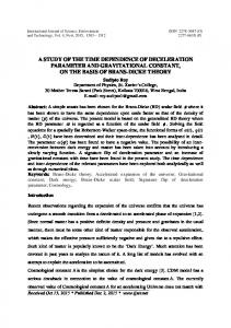
u and v are initially non-zero in complementary regions in the interior of Ω = (0, 1). Figure 1 (c) shows the third species w, which is an intermediate of the reaction pathway with two reactions. It grows from zero initially to a positive steady-state value, reflecting the fact that the slower second reaction cannot consume it faster than it is created. Figure 1 (d) shows the plot of the reaction rate q = λuv vs. (x, t). We observe that q is zero in most of the domain, as either u or v are zero there. But q is large at the interfaces of the regions where either u or v dominate, as a result of the diffusion that moves u and v from their regions of dominance and brings them in contact at the interfaces of these regions. Notice that w is thus only created at the localized interfaces, but is then present throughout Ω, as seen in Figure 1 (c), solely due to its diffusion. We also see in Figure 1 (d) that for larger times only one spike exists for q compared to three at the initial time. The waterfall plot in Figure 1 (d) provides information about the location of the interface between regions of dominance by u or v only at selected points in time. To visualize the interface and its movement over time more clearly, Figure 1 (e) plots its location for all time steps in the numerical study 0 ≤ t ≤ 20. We can see that the interface moves slowly and smoothly to its steady-state value of x∗ ≈ 0.6. To get a clearer picture of the interface movement for small times, Figure 1 (f) zooms in on the time span 0 ≤ t ≤ 0.1. This confirms that the three interfaces present initially are located at x = 0.25, 0.50, and 0.75. Figure 1 (f) shows how quickly the three interfaces coalesce to one. This makes it clear that one of the most interesting features of this problem is the behavior of the concentration interfaces between regions dominated by either u or v, which is why we refer to this problem as the interface problem. Figure 2 shows the simulation results for the model with reaction coefficient λ = 109 , with plots arranged analogously to Figure 1. Notice in Figure 2 (d), the reaction rate spikes are now higher and narrower than seen for the reaction coefficient λ = 106 . This is expected given that the value λ = 109 results in a scaling of width ε = 0.001 with height 1/ε = 1,000, compared with width ε = 0.01 and height 1/ε = 100 for λ = 106 . Notice that on the scale of Figure 2 (d) we cannot tell the height of q at latter times t when approaching the steady-state. Therefore, Figure 2 (e) and (f) are again designed to provide the detailed insight into the evolution of the reactant interfaces. Comparing their plots in Figures 1 and 2, we observe that the interfaces behave very similarly for both λ values. Motivated by the the similarity of the plots of the concentration interfaces shown in Figures 1 and 2, Figure 3 shows overlays of these interfaces for both reaction coefficients λ = 106 and λ = 109 in the (x, t)-plane. For each value of λ, results from two numerical studies are shown to ensure reliability of the results. The top four plots in the figure overlay the cases in progressively decreasing time spans. The left bottom plot shows the movement of the left portion of the interface zoomed into 0.3 ≤ x ≤ 0.5 and 0.005 ≤ t ≤ 0.014. The right bottom plot of Figure 3 shows the movement of the right portion of the interface

(a) u vs. (x, t)

(b) v vs. (x, t)

(c) w vs. (x, t)

(d) q = λuv vs. (x, t)

(e) interface vs. (x, t)

(f) zoomed interface vs. (x, t)

Simulation results for the interface problem with λ = 106 . (a), (b), (c) Concentrations u, v, w vs. (x, t), respectively. (d) Reaction rate q = λuv vs. (x, t). (e) Concentration interface in the (x, t)-plane for the entire time span 0 ≤ t ≤ 20. (f) Concentration interface in the (x, t)-plane zoomed into the time span 0 ≤ t ≤ 0.1. These studies used N = 210 + 1 mesh points, and absolute and relative ODE tolerances of 10−4 both.

Figure 1:

(a) u vs. (x, t)

(b) v vs. (x, t)

(c) w vs. (x, t)

(d) q = λuv vs. (x, t)

(e) interface vs. (x, t)

(f) zoomed interface vs. (x, t)

Simulation results for the interface problem with λ = 109 . (a), (b), (c) Concentrations u, v, w vs. (x, t), respectively. (d) Reaction rate q = λuv vs. (x, t). (e) Concentration interface in the (x, t)-plane for the entire time span 0 ≤ t ≤ 20. (f) Concentration interface in the (x, t)-plane zoomed into the time span 0 ≤ t ≤ 0.1. These studies used N = 210 + 1 mesh points, and absolute and relative ODE tolerances of 10−8 and 10−6 , respectively.

Figure 2:

zoomed into 0.5 ≤ x ≤ 0.7 and 0.05 ≤ t ≤ 0.95. We see in Figure 3 that the computed solution representing the motion of the concentration interfaces for λ = 106 and λ = 109 are very close in every time span and zoom view. In [1], it was shown analytically for the stationary problem (5) that the error between the limit solution and a solution for finite λ is uniformly on the order of ε = λ−1/3 . The present computational results show that the same estimate appears to hold for the transient problem (2). Therefore, the main conclusion of this numerical approach to asymptotic analysis is that the solution to the problem is near the asymptotic limit λ → ∞ already for the value λ = 106 . This is useful for instance for further numerical studies for this problem, because we know now that using λ = 106 is sufficient to simulate the crucial features of this problem reliably and efficiently. In Section 2, we explain the numerical method used to compute the solutions presented and identify the parameters that are studied to ensure the reliability of the solutions. In Section 3, we summarize the results of numerical parameter studies guaranteeing the accuracy and reliability of the solution over absolute and relative ODE tolerances and varying mesh resolutions.

2

Numerical Method

The interface problem (2)–(4) is spatially discretized by the finite difference method within a method of lines approach. We define a mesh with N nodes across the spatial domain Ω = [0, 1] by xj = (j − 1) ∆x for j = 1, . . . , N with uniform mesh spacing ∆x = 1/(N − 1). Then, let uj (t), vj (t), wj (t) denote approximations to u(xj , t), v(xj , t), w(xj , t), respectively. At each node xj , j = 1, . . . , N , a finite difference discretizes the spatial derivatives, still leaving the time dependence of all quantities. To write this system of ordinary differential equations (ODEs) for functions uj (t), vj (t), wj (t) in vector form, define the three vector functions U (t) := [u1 , . . . , uN ]T , V (t) := [v1 , . . . , vN ]T , and W (t) := [w1 , . . . , wN ]T , each with N components. We organize the equations for the vector U in system form dU = −K (u) y + r(u) (U, V, W ), dt

0 < t ≤ tfin ,

(7)

with initial condition U (0) = Uini . Here, K (u) ∈ RN ×N denotes the species stiffness matrix resulting from the discretization of the diffusion term and r(u) ∈ RN the discretization of the reaction terms. Similarly, we derive analogous ODE systems for the other concentration vectors V and W . A more detailed explanation of the choices in the finite difference discretization, in particular of the handling of the boundary conditions, is contained in [6, Appendix A]. Combining the three species concentration vectors into a vector function y(t) := [U T , V T , W T ]T with 3N components allows the problem to be posed as a single ODE system in standard form dy = f (t, y), dt

0 < t ≤ tfin ,

y(0) = yini ,

(8)

T T T T where yini := [Uini , Vini , Wini ] and f (t, y) = −K y + r(y) with  (u)   (u)  K r  , r(y) =  r(v)  (9) K= K (v) K (w) r(w)

from (7) and the analogous ODE systems for V and W . We note that the stiffness matrix K ∈ R3N ×3N is seen to be constant with non-negative diagonal and nonpositive off-diagonal entries, but is not symmetric. We also point out that each component of the vector function r(y) depends in general on all three vectors of unknowns U (t), V (t) and W (t). To guarantee the reliability of numerical simulations, several key numerical parameters need to be carefully varied over a range of possible values to give confidence in the numerical results. Since we do not know a priori where the internal layers are located and in order not to bias the numerical method towards any region, we use a uniform spatial mesh. To obtain a reliable spatial discretization, a sufficient number of spatial mesh points N are needed. To select the number N , we use the rule-of-thumb that the numerical mesh should have an order of magnitude more points than the size of the region of the internal layers. As a guide, the asymptotic analysis of the internal layer in the stationary problem leads us to expect a width of ε = λ−1/3 for the internal layer. Therefore for λ = 106 , this yields ε = 0.01. The requirement that the mesh spacing ∆x be an order of magnitude smaller than the scaling ε width leads us to require ∆x = 1/1024 ≈ 0.001, resulting in the choice N = 210 + 1 = 1025 for λ = 106 . Simulations with this relatively coarse mesh in one spatial dimension are cheap and easily enable extensive parameter studies of the problem. By contrast, for λ = 109 , we have ε = 0.001 and the requirement from the rule-ofthumb gives us a mesh size with N = 212 + 1 = 8193 points, for which numerical simulations are comparably expensive. On the one hand, this explains the importance of our result in Section 1 that the problem is already in its asymptotic limit for λ = 106 and that simulations for this significantly cheaper parameter value suffice. On the other hand, we still need to demonstrate that the simulation results used to draw this conclusion in Section 1 are reliable. This is shown by the results in Section 3 that carefully compare studies for λ = 109 across a range of values N . Since the problem (2)–(4) has significant transients in time, it is vital for efficient simulations that the ODE solver vary its time steps such that they are small during the temporal transient for accuracy and large outside of the transients for efficiency. To this end, we use Matlab’s ode15s function, which is an implementation of the Numerical Differentiation Formulas (NDFk) [3], a generalization of the well-known Backward Differentiation Formulas (BDFk). Both methods are families of methods with variable method order 1 ≤ k ≤ 5 and suitable for the solution of stiff ODE systems as they arise from method of lines discretizations of reaction-diffusion equations. ODE methods for stiff systems must necessarily use implicit time discretizations. The implementation

in ode15s includes sophisticated automatic method order and step size selection, based on estimating the local error of the computed at every time step [3]. The user has control over the absolute and relative tolerance demanded of this error estimator, where tighter tolerances are expected to result in higher accuracy of the solution at the expense of smaller time steps and more costly simulations. Therefore, we have an interest in not selecting the tolerances unnecessarily tight, but rather we wish to find the coarsest tolerances possible for efficiency that still give reliable numerical results. Careful studies in [6] analyzed the behavior of the numerical method and the reliability of the solution across various ODE absolute and relative tolerance values for both relevant values λ = 106 and λ = 109 over a range of numbers of spatial mesh points N . These studies guarantee the reliability of the simulations with the values used in Figures 1 through 3. and these result validate the use of the numerical solutions in our comparisons in Section 1.

3

Numerical Parameter Studies

The numerical solution of a problem involving an asymptotic parameter poses great risks, as numerical methods are by their nature designed for problems whose solutions and crucial quantities vary smoothly. But it is inherent to asymptotic analysis that crucial quantities become large or small as the asymptotic parameter increases towards its asymptotic limit. Thus, to draw conclusions for the asymptotic behavior of the model based on numerical studies, we need to ensure the accuracy and reliability of the numerical results for each fixed value of the asymptotic parameter. We approach this issue here by presenting the results of systematic studies of the numerical parameters that control the accuracy of the numerical method. While this should always be done before trusting numerical results, this, as well as its explicit inclusion in this paper, is particularly pertinent in the context of asymptotic analysis. Numerical parameter studies for both values of λ = 106 and λ = 109 in [6] analyzed which choices of ODE tolerances resulted in reliable numerical results for each fixed value of the mesh resolution N . These studies were performed for a range of spatial mesh resolutions N = 2ν + 1 with ν = 9, 10, 11, 12 and varied the values of both absolute and relative across relative (rel) and absolute (abs) ODE tolerances. For λ = 106 , the data in [6, Table 1] shows that the numerical method is successful for relative tolerance values tighter than or equal to 10−3 for all the values of the absolute tolerance at least as tight as 10−1 . For λ = 109 , we observed in [6, Table 3] that the ODE solver breaks down before reaching the final time tfin = 20 for the coarsest relative tolerances 10−2 and 10−4 attempted. The breakdown for these coarse tolerances is due to the time step not being permitted to decreased below the minimum value allowed. However, the numerical method begins to succeed for relative tolerance values tighter than or equal to 10−6 for all the values of the absolute tolerance tighter than 10−2 .

We also observed in [6, Table 3] that the computation time approximately doubles for every doubling of the mesh resolution N . This explains our interest in analyzing if reliable results can be obtained for coarser mesh resolutions than the N = 8193 suggested by the rule-ofthumb discussed in Section 2. If the solution is already reliable for coarser mesh resolutions such as N = 1025, this offers an approach to cheaper numerical simulations for λ = 109 . Thus, it is the purpose of the present section to compare the crucial features of the solution of the interface problem for λ = 109 across a range of mesh resolutions N . Following the accuracy study of the interface solutions for convergent cases of [6, Table 3], we focus here on a selected range of parameter values of the relative and absolute ODE tolerances, namely the ones used in Figure 3. That is, we keep the relative tolerance 10−6 and absolute tolerance 10−8 fixed for each mesh size N = 2ν + 1 for ν = 9, 10, 11, 12, and we now check the accuracy of the solution by considering plots of the concentration interface motion as crucial feature of the interface problem. Figure 4 shows plots of the concentration interface in the (x, t)-plane for the reaction coefficient λ = 109 . The top four plots overlay the cases of all N for comparison in progressively decreasing time spans. The left bottom plot shows the movement of the portion of the interface zoomed into 0.3 ≤ x ≤ 0.5 and 0.005 ≤ t ≤ 0.014. The right bottom plot shows the movement of the portion of the interface zoomed into 0.5 ≤ x ≤ 0.7 and 0.05 ≤ t ≤ 0.95. We observe that the interface results for each mesh refinement track closely with each other in every time span and zoomed view. Therefore, we see no significant change in accuracy and the simulations for λ = 109 are confirmed to be reliable already for N = 1025, as used in the results in Section 1. Analogous results are obtained for the relative tolerance 10−8 and absolute tolerance 10−8 , the other set of values used in Figure 3.

References [1] L. V. Kalachev and T. I. Seidman. Singular perturbation analysis of a stationary diffusion/reaction system whose solution exhibits a corner-type behavior in the interior of the domain. J. Math. Anal. Appl., 288:722–743, 2003. [2] T. I. Seidman and L. V. Kalachev. A one-dimensional reaction/diffusion system with a fast reaction. J. Math. Anal. Appl., 209:392–414, 1997. [3] L. F. Shampine and M. W. Reichelt. The MATLAB ODE suite. SIAM J. Sci. Comput., 18(1):1–22, 1997. [4] A. M. Soane, M. K. Gobbert, and T. I. Seidman. Design of an effective numerical method for a reaction-diffusion system with internal and transient layers. Technical Report number 2006, Institute for Mathematics and its Applications, University of Minnesota, 2004. [5] A. M. Soane, M. K. Gobbert, and T. I. Seidman. Numerical exploration of a system of reaction-diffusion equations with internal and transient layers. Nonlinear Anal.: Real World Appl., 6(5):914–934, 2005. [6] Y. Yang, M. Muscedere, and M. K. Gobbert. Numerical studies of the asymptotic behavior of a reaction-diffusion system with a fast reaction. Technical Report TR2008–4, Department of Mathematics and Statistics, University of Maryland, Baltimore County, 2008.

Simulation results of the concentration interface for both reaction coefficients λ = 106 and λ = 109 in the (x, t)-plane. The top four plots overlay these cases for comparison in progressively decreasing time spans. The left bottom plot shows the movement of the left portion of the interface zoomed into 0.3 ≤ x ≤ 0.5 and 0.005 ≤ t ≤ 0.014. The right bottom plot shows the movement of the right portion of the interface zoomed into 0.5 ≤ x ≤ 0.7 and 0.05 ≤ t ≤ 0.95. A mesh size of N = 210 + 1 is used for both values of λ. The data shown for λ = 106 used an absolute ODE tolerance of 10−4 and relative tolerances of 10−3 and 10−4 . The data shown for λ = 109 used an absolute ODE tolerance of 10−8 and relative tolerances 10−6 and 10−8 .

Figure 3:

Simulation results of the concentration interface for reaction coefficients λ = 109 in the (x, t)-plane comparing cases of mesh size N = 2ν + 1 for ν = 9, 10, 11, 12. The top four plots overlay these cases for comparison in progressively decreasing time spans. The left bottom plot shows the movement of the left portion of the interface zoomed into 0.3 ≤ x ≤ 0.5 and 0.005 ≤ t ≤ 0.014. The right bottom plot shows the movement of the right portion of the interface zoomed into 0.5 ≤ x ≤ 0.7 and 0.05 ≤ t ≤ 0.95. Constant values for the absolute tolerance 10−8 and relative tolerance 10−6 are used.

Figure 4: