Diaz-Ramirez, J., Camacho, R., McAnally, W. and Martin, J. (2012). Parameter uncertainty methods in evaluating a lumped hydrological model. Obras y Proyectos 12, 42-56
Parameter uncertainty methods in evaluating a lumped hydrological model Método de incertidumbre paramétrica en la evaluación de un modelo hidrológico agregado Fecha de entrega: 8 de octubre 2012 Fecha de aceptación: 12 de diciembre 2012
Jairo Diaz-Ramirez, Rene Camacho, William McAnally and James Martin Department of Civil and Environmental Engineering, Mississippi State University, 501 Hardy Road, 235 Walker Engineering Bldg., Box 9546, Mississippi 39762-9546, USA,
[email protected],
[email protected],
[email protected],
[email protected]
Water resources modelers face the challenge of dealing with numerous uncertainties due to the lack of knowledge of the natural systems, numerical approaches used in modeling (equations, parameters, structures, solutions), and field data collected to set up and evaluate models. Propagation of parameter uncertainty into model results is a relevant topic in environmental hydrology. Uncertainty analyses improve assessment of hydrological modeling. There is a need in modern hydrology of developing and testing uncertainty analysis methods that support hydrological model evaluation. In this research the propagation of model parameter uncertainty into streamflow model results is evaluated. The Hydrological Simulation Program – FORTRAN (HSPF) supported by the US Environmental Protection Agency was evaluated using hydroenvironmental data from the Luxapallila Creek watershed located in Mississippi and Alabama, USA. The uncertainty bounds of model outputs were computed using the Monte Carlo simulation and Harr’s point estimation methods. Analysis of parameter uncertainty propagation on streamflow simulations from 12 HSPF parameters was accomplished using 5,000 Monte Carlo random samples and 24 Harr selected points for each selected parameter. The comparison showed that Harr’s method could be an appropriate initial indicator of parameter uncertainty propagation on streamflow simulations, particularly for hydrology models with several parameters. Keywords: HSPF, parameter uncertainty, Monte Carlo simulation, Harr’s point estimation method, uncertainty bounds of streamflow simulations
42
Los modeladores de recursos hídricos enfrentan el desafío de trabajar con diferentes tipos de incertidumbre debido a la falta de un completo conocimiento de los sistemas naturales, procesos de modelación, aproximaciones numéricas (ecuaciones, parámetros, estructuras, soluciones), y datos de terreno tomados para desarrollar y evaluar modelos. La propagación de la incertidumbre paramétrica en los resultados de las simulaciones es un tópico relevante en la hidrología ambiental. Los análisis de incertidumbre mejoran la evaluación en el modelamiento hidrológico. Existe una necesidad en la hidrología moderna de desarrollar y evaluar métodos de análisis de incertidumbre que apoyen la evaluación de los modelos hidrológicos. En esta investigación se evaluó la propagación de la incertidumbre de los parámetros de un modelo en los resultados del flujo simulado. Un programa de simulación hidrológico HSPF patrocinado por la Agencia Ambiental de los EE.UU., fue evaluado utilizando datos hidroambientales de la cuenca de la quebrada Luxapallila localizada en los estados de Misisipi y Alabama, EE.UU. Los límites de incertidumbre de las salidas del modelo fueron calculados utilizando los métodos de simulación Monte Carlo y el método probabilístico de estimación puntual de Harr. El análisis de la propagación de la incertidumbre paramétrica en simulaciones de caudales con HSPF utilizando 12 parámetros fue realizada con 5000 muestras aleatorias de Monte Carlo y 24 puntos seleccionados de Harr para cada parámetro evaluado. La comparación mostró que el método de Harr podría ser un indicador inicial apropiado de la propagación de la incertidumbre paramétrica en simulaciones de caudales, particularmente en modelos hidrológicos con varios parámetros. Palabras clave: HSPF, incertidumbre paramétrica, simulación Monte Carlo, método de estimación puntal de Harr, límites de incertidumbre de simulaciones de caudales
Diaz-Ramirez, J., Camacho, R., McAnally, W. and Martin, J. (2012). Obras y Proyectos 12, 42-56
Introduction
Hydrologic models are represented by a series of input data (e.g. precipitation and evaporation), parameters (e.g. soil, land use, and channel properties), and structure (e.g. black-box, conceptual, physically based, grid, and lumped models). Every component of hydrologic models depicts uncertainty due to the lack of knowledge about real systems. Uncertainty in input data is due to natural variability, measurement inaccuracy, and errors in handling and processing data (Melching, 1995). Model parameters and structure show uncertainty due to model assumptions and approximations, scale effects, and variability of inputs and parameters in time and space (Gupta et al., 2005; Tung, 1996). The uncertainty of input data on model results has been studied separately from model parameter uncertainty (Souid, 1999). Georgakakos et al. (2004) pointed out that few studies have investigated model structure uncertainty. Butts et al. (2004) declared that uncertainty evaluation is compensated among components (input data, model parameters, and model structure) because they are strongly interlinked. The identification, quantification, and reporting of the different sources of errors in a modeling process constitute an uncertainty analysis (McIntyre et al., 2002; Refsgaard and Henriksen 2004; Refsgaard et al., 2007). Uncertainty analysis has received considerable attention during the last two decades by the water resources community. In hydrological modeling, important progress has been observed in the identification and understanding of the different sources of uncertainty, as well as in the incorporation of strategies for their quantification (e.g. Butts et al., 2004; Georgakakos et al., 2004; Wagener et al., 2003). Uncertainty analysis of computer-based models is a valuable tool to do the following: understand the inability of a model to accurately and precisely depict the real world; enhance the value of information reported; distinguish between bias and precision error; calculate the precision limit of results; identify which components are most and least important; determine where to place more effort/resources to decrease the total uncertainty of the output; re-build a model; understand model limitations and strengths; calculate statistical properties of a model output; determine reliability analysis; and compare and choose between models (Morgan and Henrion, 1990;
Tung, 1996; Tung and Yen, 2005). Techniques applicable for evaluating error propagation from different sources on hydrology model results can be classified in three groups: first-order methods (Melching, 1992, 1995; Zhang and Yu, 2004); probabilistic point estimate methods (Harr, 1989; Rosenblueth, 1975; Tung and Yen, 2005; Yu et al., 2001;); and Monte Carlo based methods such as Bayesian analysis, Markov Chain Monte Carlo, and the Generalized Likelihood Uncertainty Estimation method (Beven and Binley, 1992; Dilks et al. 1992; Thiemann et al., 2001). Applications and comparisons of these techniques on hydrology models can be found in Rogers et al. (1985), Binley et al. (1991), Melching (1995), and Yu et al. (2001). In general, these studies assumed that the results of the Monte Carlo method were most reliable when estimations from other uncertainty methods were compared. The Monte Carlo simulation is the best known and simplest way of sampling the entire range of likely observations of the system being studied (Morgan and Henrion, 1990). Most of the firstorder and probabilistic point estimate methods are more computationally efficient than the Monte Carlo method. Melching (1995) pointed out that “research is needed to define strengths and weaknesses of applying these methods to computer models of watershed hydrology.” Numerous real world hydrologic models exist, e.g. continuous or event based, distributed or lumped parameters, and empirical or physical equations (Singh, 1995; Singh and Woolhiser, 2002; Singh and Frevert, 2002). Currently many continuous hydrologic models are set up in conjunction with Geographical Information Systems GIS. In 1996, the US Environmental Protection Agency EPA released the Better Assessment Science Integrating Point and Nonpoint Sources – BASINS, which links the Hydrological Simulation Program – FORTRAN HSPF (Bicknell et al., 2001) and other watershed and water quality models with a GIS software, MapWindow (USEPA, 2011). Also BASINS incorporates an extensive U.S. data base (i.e. land use, climatological and water quality data) graphical and statistical analysis, and reporting tools. The HSPF software is a continuous, reservoir-type, semidistributed parameter model supported by the USEPA. The HSPF model is one of the most comprehensive, flexible and modular programs of watershed hydrology and water
43
Diaz-Ramirez, J., Camacho, R., McAnally, W. and Martin, J. (2012). Parameter uncertainty methods in evaluating a lumped hydrological model. Obras y Proyectos 12, 42-56
quality available (Donigian et al., 1995). HSPF has been applied in different zones around the world since the 1980’s (Diaz-Ramirez et al., 2008, 2011; Donigian et al., 1995; Singh and Woolhiser, 2002). Applications of HSPF in watersheds in the southeastern United States can be found in Alarcon et al. (2009), Diaz-Ramirez et al. (2011), and Duan et al. (2008). These studies mainly analyzed hydrological processes on the Luxapallila Creek watershed (Alabama and Mississippi), Saint Louis Bay watershed (Mississippi), Fish River watershed (Alabama), and the Mobile Bay basin (Alabama, Mississippi, Tennessee, and Georgia). The main goal of this study is to evaluate two uncertainty methods, the Monte Carlo method and Harr’s probabilistic point estimate method, in propagating HSPF parameter uncertainty into daily streamflow model results. Physical data from the Luxapallila Creek watershed are used to set up the HSPF model. This watershed is located in Alabama and Mississippi, USA. U.S. Geological Survey USGS streamflow data collected at the watershed outlet from 01/01/2002 to 12/31/2005 were used to evaluate model results.
The HSPF model The Hydrological Simulation Program – FORTRAN HSPF model (Bicknell et al., 2001) computes the movement of water through a complete hydrologic cycle – precipitation (rain/snow), evapotranspiration, runoff, infiltration, and flow through the ground – and the associated transport of constituents with that flow. It represents a watershed as a collection of land segments and channels (reaches). The land segments, either pervious or impervious, are connected to other land segments or to channel reaches, which can function as either streams or reservoirs. Rainfall is computed over the entire watershed and runs off land segments and reaches. Pervious land segments also store water in the plant canopy, on the surface, and in the soil, from which it can percolate into groundwater or flow down slope as interflow. Water in the plant canopy, surface, and surface soil layers can be lost to evapotranspiration. Water in reaches can be lost to evaporation, but not to groundwater. Water can flow from a land segment to a reach or to another land segment. Water in a reach must
44
either be stored there or flow into another reach; it cannot flow onto land except by irrigation. Table 1 describes HSPF parameters and their ranges related to hydrology in areas without snow. The current HSPF application is in the Luxapallila Creek watershed, Alabama/Mississippi where climate is classified as humid subtropical. The most probable HSPF values in the Luxapallila Creek watershed were extracted from an 18-year (1985-2003) model evaluation performed by McAnally et al. (2006). The model tested by McAnally et al. (2006) was manually calibrated using guidelines provided by HSPF developers (USEPA, 2012) and explained more than 72% of the daily variability of streamflows. Coefficient of determination R2 and Nash-Sutcliffe NS statistics were good on daily (R2 = 0.72 and NS = 0.72) and monthly (R2 = 0.84 and NS = 0.84) periods. The model was evaluated under a large range of streamflows (0.8 m3/s to 566 m3/s). Table 1 also shows the impact of each HSPF parameter on modeling hydrologic processes. The impact of every HSPF parameter on hydrologic processes is based on guidelines provided by HSPF developers (USEPA, 2012). These guidelines provide advice on which parameter to modify, and in what direction, in order to accomplish a particular hydrologic process evaluation (water balance, high/low flow distribution, storm flow, and seasonal discrepancies). The HSPF model also computes the transport and kinetics of multiple water quality constituents, including temperature, sediment, nutrients, and pesticides. As such, it presents a nearly complete package for modeling hydrology and water quality of a watershed. A more complete description of features and capabilities can be found in the HSPF user’s manual (Bicknell et al., 2001). Some versions of HSPF can be run in standalone mode, but the EPA-supported version is run through a BASINS interface, WinHSPF (USEPA, 2011). The rainfall-runoff model HSPF requires specific inputs that BASINS can generate. Watershed delineation tools within BASINS enable the user to automatically or manually generate a watershed drainage network and subnetworks, each consisting of land segments and receiving water reaches. The literature review reports several deterministic applications of the HSPF model (Moore et al., 1988; Laroche et al., 1996; Al-Abed and Whiteley, 2002; Hayashi et al., 2004; Albek et al., 2004; Nasr et al., 2007; Diaz-
Diaz-Ramirez, J., Camacho, R., McAnally, W. and Martin, J. (2012). Obras y Proyectos 12, 42-56
Table 1: HSPF parameter definition and range (USEPA, 2000); most probable value for Luxapallila Creek watershed simulations (McAnally et al., 2006); and hydrologic processes impacted by each parameter marked with X (USEPA, 2012)
Range
most probable water balance value
Hydrologic Process high/ low flow distribution
storm flow
X
X
Name
Definition
LZSN mm
Lower zone nominal soil moisture storage
50.8 -381.0
228.6
X
INFILT mm/hr
Index to infiltration capacity
0.025 – 12.7
2.8
X
KVARY 1/mm
Variable groundwater recession
0.0 – 127.0
45.7
AGWRC
Base groundwater recession
0.92 - 0.999
0.997
DEEPFR
Fraction of groundwater inflow to deep recharge
0.0 - 0.5
0.2
BASETP
Fraction of remaining evapotranspiration from baseflow
0.0 - 0.2
0.04
AGWETP
Fraction of remaining evapotranspiration from active groundwater
0.0 - 0.2
0.025
X
seasonal discrepancies
X X X
X X
X
CEPSC mm
Interception storage capacity
0.0 – 10.2
3.8
X
UZSN mm
Upper zone nominal soil moisture storage
1.27 – 50.8
27.9
X
INTFW
Interflow inflow parameter
1.0 - 10.0
3.0
X
IRC
Interflow recession parameter
0.3 - 0.85
0.6
X
LZETP
Lower zone evapotranspiration parameter
0.0 - 0.9
0.1
Ramirez et al., 2008); however few applications attempt to quantify propagation of parameter, input data, and/ or structure uncertainty into model results. Paul (2003) evaluated the effect of parameter uncertainty in the HSPF model to predict in-stream bacterial concentrations using First Order Analysis FOA techniques. He evaluated 10 water quality parameters from pervious and impervious areas and three in-stream water quality parameters. However, he did not evaluate the uncertainty effects of hydrologic/hydraulic parameters on modeling fecal coliform and assumed that the hydrology and hydraulic of the model were well calibrated. Paul (2003) pointed out that water quality parameters from pervious and impervious areas carried on most of the parameter uncertainty in simulated in-stream bacterial concentrations. In particular, the maximum storage of bacteria on pervious land surface parameter contributed with 99.86% of the variance in simulated peak in-stream concentration of fecal coliform
X
X
concentration in-stream. The contribution of the three instream water quality parameters to the output variance was negligible (0.12%). In addition, he recommended further research to evaluate the effects of hydrology and hydraulic processes on in-stream fecal coliform simulations. Jia (2004) investigated parameter uncertainties in the HSPF model applying the generalized likelihood uncertainty estimation GLUE approach. A Latin hypercube sampling technique was used to generate random multiple parameter sets. The GLUE method introduced by Beven and Binley (1992) is a Monte Carlo based strategy for evaluation of parametric uncertainty. GLUE accepts multiple sets of parameter values as equal likely representations of a physical system. Other sources of uncertainty such as model structure and input data are treated implicitly within the GLUE framework. Unlike the formal methods for Bayesian inference, GLUE uses “informal” likelihood functions which are formulated without considering the
45
Diaz-Ramirez, J., Camacho, R., McAnally, W. and Martin, J. (2012). Parameter uncertainty methods in evaluating a lumped hydrological model. Obras y Proyectos 12, 42-56
structure of the residuals between the observations and the model simulations of a given state variable. Therefore, any measure of goodness of fit such as the Nash and Sutcliffe efficiency criterion, or the total sum of the errors can be implemented in the GLUE methodology (Beven and Binley 1992). Jia (2004) evaluated seven hydrologic parameters at the watershed outlet (i.e. LZSN, INFILT, AGWRC, DEEPFR, UZSN, and IRC). After 50000 HSPF runs, many acceptable parameter sets were identified by the GLUE approach. Information on the total runoff distribution was not available, and wide variations of the total runoff (i.e. surface runoff, interflow, and baseflow) were acceptable. Wu (2004) assessed the propagation of parameter uncertainty in both HSPF and CE-QUAL-W2 models using First-Order Error Analysis FOEA. He pointed out that the uncertainty in parameters related to streamflow generation was the main source of variance in simulated nutrient loads. However, when simulated nutrient concentrations were analyzed, some parameters related to hydrology processes have no significant effect. The author justified this difference by the non-linear relationship between pollutant loads and their concentrations. So, FOEA may not be an appropriate method to analyze propagation of parameter uncertainty in complex models. Wu recommends more analysis between FOEA and Monte Carlo analysis.
Harr and Monte Carlo methods
Uncertainty analysis methods used in hydrology simulation can be arranged in three groups: first-order methods, probabilistic point estimation methods, and Monte Carlo based methods. In this study, the Harr probabilistic point method and Monte Carlo method are used to propagate parameter uncertainty into HSPF streamflow simulations. The concept of probability point estimate methods PPEMs was originated by Rosenblueth (1975). A PPEM propagates the parameter uncertainty by performing point estimations of the function without calculating the derivatives of the function (first-order methods). Selected point estimations of model parameters are calculated using statistical moments (typically the mean and variance) of the variables instead of computing the entire probability density function PDF of the model parameters (as performed by Monte Carlo simulations). Harr (1989) developed a PPEM using the principal component matrix theory. This method
46
considers the mean, standard deviation, and correlation of the parameters. The Harr method propagates the parameter uncertainty through model outputs by performing two point estimations of the parameter space. The correlation matrix of parameters, C, is decomposed as
(1)
where e is the eigenvector matrix; λ is the diagonal eigenvalue matrix and eT is the transpose of the eigenvector matrix. Thus, someone using Harr’s method must generate the correlation matrix of selected parameters and then compute, using mathematical programs such as MATLAB, the eigenvector matrix and the diagonal eigenvalue matrix. The uncorrelated and standardized coordinates can be calculated by
where μ is the vector of the expected values of the parameter; n is the number of parameters; σ is the diagonal matrix of the standard deviation of the parameters; and ei is the eigenvalue λi. Finally, based on the two coordinates selected along each eigenvector (2a) and (2b), the user must compute the corresponding model output values. For instance, this research used 12 HSPF parameters; thus 24 coordinates were calculated and 24 model outputs were generated for each simulated day. Then, the 95th and 5th percentiles of these 24 model outputs were calculated to generate the 90% uncertainty bounds of model outputs using the percentile function in MATLAB. As a summary, the Harr method involves the following steps:
1. Identify model parameter ranges and sample values of each parameter;
2. verify the symmetry of each input parameter (if the distribution is not symmetric, the Harr method is not appropriate. However, parameter transformation could be performed to ensure input parameters are symmetric);
3. compute mean and standard deviation of each parameter;
Diaz-Ramirez, J., Camacho, R., McAnally, W. and Martin, J. (2012). Obras y Proyectos 12, 42-56
4. calculate the correlation matrix of each parameter; 5. determine eigenvectors from the correlation matrix;
4. repeat steps 2 and 3 many times; and 5. analyze the model outputs (e.g., CDF, percentiles, mean, standard deviation, etc.).
6. compute 2n coordinate points using equations (2a) and (2b);
7. evaluate the model with parameter values computed in step 6;
8. analyze the model outputs (percentiles, mean, standard deviation, etc). A drawback of the Harr method is that the uncorrelated and standardized coordinates may fall outside the parameter bounds (Christian and Baecher, 2002). In this study, when a coordinate was outside the pre-established HSPF parameter range, the closest parameter limit was used instead of the outside value. This issue can be related to poor definition of model parameter range. However, HSPF hydrologic algorithms have been tested since 1960 and model developers have developed a comprehensive list of parameter ranges (USEPA, 2000). An application of the Harr method in simulating watershed hydrology is found in Yu et al. (2001). The Monte Carlo method computes an empirical probability distribution of the model output using random values for the input variables sampled from their probability distribution (Metropolis and Ulam, 1949). Detailed information on Monte Carlo simulation is found in Ronen (1988), Morgan and Henrion (1990), and Sobol’ (1994). The Monte Carlo simulation is the best known uncertainty method, and the simplest way of sampling the entire range of likely observations of the system being studied (Morgan and Henrion, 1990). Melching (1995) declared that the Monte Carlo method “may be the only method that can estimate the cumulative density function CDF and PDF of Z (a model parameter) for cases with highly nonlinear and/or complex system relationships.” The Monte Carlo simulation involves five steps:
1. Generate probability distributions of selected model parameters (e.g., normal, triangular, beta, etc.);
2. calculate a random value from the parameter’s distributions;
3. evaluate the model using the random value calculated in step 2;
The Monte Carlo simulation has been applied to study the uncertainty of forcing input data and model parameters in computer models of watershed hydrology (Melching, 1995; Carpenter and Georgakakos, 2004). Melching (1995) stated that “for complex, nonlinear models with many uncertainty basic variables, however, the number of simulations (thus the computer time) necessary to achieve an accurate estimate may become prohibitive.” Increasing of computer processing speeds makes computations more tractable. Monte Carlo method results have been used as a baseline when comparisons with other uncertainty methods have been done (Binley et al., 1991; Melching, 1992; Melching, 1995; Yu et al., 2001). In summary, the Harr method is computationally more efficient than the Monte Carlo method. In Harr’s method, mean, standard deviation of parameters and their correlations are used to propagate parameter uncertainty into model results. The Harr method is limited to symmetrical distributions and sometimes the uncorrelated and standardized coordinates are calculated out of the parameter bounds. The computation algorithm of the Monte Carlo method has a simple structure and is used in complex and nonlinear models. In the Monte Carlo method, random parameter inputs are computed from their probability distributions and are then propagated through model results. The Monte Carlo method is computationally time consuming at high levels of accuracy.
Methodology Study area
This study used physical data from the Luxapallila Creek watershed located in the Southeastern of United States. The watershed flows through Fayette, Lamar, Marion, and Pickens counties in Alabama and into Lowndes and Monroe counties in Mississippi (Figure 1). Near the outlet (USGS Station 02443500), the watershed has a drainage area of 1.801 km2, an average basin slope of 2%, and average annual precipitation (1982 - 2004) of 1.379 mm recorded at the Millport 2E weather station. Seasonal fluctuations in rainfall result in maximum river discharges
47
Diaz-Ramirez, J., Camacho, R., McAnally, W. and Martin, J. (2012). Parameter uncertainty methods in evaluating a lumped hydrological model. Obras y Proyectos 12, 42-56
from January to April and minimum discharges from August to September. Elevation in the study area ranges from 45 to 274 m mean sea level. The USGS Geographic Information Retrieval and Analysis System GIRAS, states that land cover developed in the early 1980’s is distributed as 73% forest land, 20% agricultural land, 6% wetlands, and 1% other land types (barren, urban, and non-urban). More information about the Luxapallila Creek watershed can be found at Diaz-Ramirez et al. (2011).
Figure 1: Location of the Luxapallila Creek watershed
HSPF model set up
The Luxapallila watershed model was set up with a standard set of procedures and data as might be used in any BASINS application to provide a HSPF input data file (uci file). Spatial and climatic time series databases, including land use, overland flow slope and length, reach characteristics, and detailed meteorological data are used as inputs to HSPF. The model was lumped using one basin area and one main channel because streamflow-gauging station data from only one station were available (USGS 2443500). Topographic data were created from the standard USGS Digital Elevation Models DEMs, and the DEMs were also used to delineate the watershed boundaries. The length and slope of overland flow and reach were calculated and kept constant throughout the simulations. Manning’s n roughness coefficients for overland flows were determined 48
by literature review and were kept constant throughout the simulations. The watershed was partitioned into five pervious and one impervious land types (Table 2). Table 2: Pervious and impervious land types simulated using 1980 GIRAS data
Land cover Forest land Agricultural land Barren land Wetlands Urban land (pervious) Urban land (impervious) Water
Surface area km2 1316.9 360.0 2.5 104.4 8.1 8.1 1.5
Surface area % 73.1 20.0 0.1 5.8 0.4 0.4 0.1
Hourly precipitation data were NEXRAD stage IV data from the Earth Observing Laboratory web page (http://data. eol.ucar.edu/codiac/dss/id=21.093). Downloaded rainfall data were uncompressed and incorporated into input files by use of the Watershed Data Management WDMUtil software (Hummel et al., 2001). Hourly potential evapotranspiration, air temperature, dew point, wind speed, solar radiation, evaporation, and cloud cover values were obtained from the Haleyville station. The weather database for the Haleyville station was downloaded from the BASINS web site. The model was run for data from 01/01/2002 through 12/31/2005. The model time step was hourly, but streamflow data were output daily to compare with observed data (USGS Station 02443500).
Computational experiment Monte Carlo method The first step in the Monte Carlo simulation MCS was to determine the probability density functions PDFs for the input parameters considered in the study. In most studies this is performed by using a non-informative uniform distribution for each parameter, which covers a feasible range of parameter values for the particular study. Due to the lack of data to estimate the PDFs, all parameters were assigned a triangular distribution, which is defined by the lowest, most probable, and highest values. Most probable values were extracted from an 18-year model calibration of the Luxapallila Creek watershed (McAnally et al., 2006), see Table 1. Highest and lowest values were
Diaz-Ramirez, J., Camacho, R., McAnally, W. and Martin, J. (2012). Obras y Proyectos 12, 42-56
assigned based on the EPA BASINS Technical Note 6 (USEPA, 2000), also in Table 1. Haan (2002) pointed out that the accuracy of the Monte Carlo simulations is a function of the assumed PDF and number of simulations performed. In selecting PDFs and number of simulations, there is no defined answer and judgment is required to make these decisions (Haan, 2002). Authors believe that taking into consideration the calibrated parameters (most probable values) from a long term deterministic evaluation (McAnally et al., 2006) in the study area will positively impact the Monte Carlo method results by forcing the parametric space search around the most probable values. Five thousand random samples from the 12 HSPF parameter’s distributions (triangular distributions) were generated using MATLAB. Then, the HSPF program was run using the selected random samples from 01/01/2002 to 12/31/2005. Finally, evaluation of streamflow simulations was accomplished (stability results, 95th and 5th percentiles) at daily levels with 5.000 streamflow simulations for each simulation day. To determine the number of realizations (stability results) sufficient to analyze the uncertainty of streamflow simulations, the values of Absolute Relative Errors ARE of simulated daily flows were calculated as N Q − Qi ARE = ∑ i +1 Qi i =1
where N is the number of Monte Carlo simulations; and Qi is the simulated daily flow for run i. For instance, in this study, 1.096 daily HSPF streamflows from 01/01/2003 through 12/31/2005 were used; this means that 1.095 ARE results were calculated for each Monte Carlo simulation.
Harr method
The first step in the Harr method was to calculate the correlation matrix, mean, and standard deviation of the 12 HSPF parameters evaluated. The USEPA developed a database of HSPF model parameters (USEPA, 2006). This database was called HSPFParm and contains HSPF parameter values of several model applications in the U.S. Twenty seven sets of parameter values were used to compute the correlation matrix, mean, and standard deviation of selected parameters. Table 3 depicts mean,
standard deviation, median, mode, and skew values of selected HSPF parameters. In a symmetric distribution, the mean, median, and mode are the same (Haan, 2002). For each parameter in Table 3, it can be observed that these three statistically measured values are close and the skew values are around zero. This means that the assumption of symmetry for input distributions in the Harr’s method is most likely valid in this study. Other uncertainties could arise in using the Harr’s method. For example, the short sets of parameter values (only 27) and the lack of parameter values found in the study site or near watersheds. Table 4 shows the correlation matrix of selected HSPF parameters. Then, the eigenvector and eigenvalue matrices from the correlation matrix were calculated using MATLAB. Table 3: Statistical measure values of selected HSPF parameters Parameter LZSN, mm INFILT, mm/hour KVARY, 1/mm AGWRC DEEPFR BASETP AGWETP CEPSC, mm UZSN, mm INTFW IRC LZETP
mean 146.7 2.0 24.3 0.97 0.04 0.02 0.02 0.3 14.8 2.9 0.7 0.3
standard median mode deviation 48.0 1.0 25.4 0.02 0.1 0.02 0.04 0.7 7.3 1.7 0.2 0.3
156.4 1.9 24.8 0.98 0.002 0.02 0.02 0.00 10.9 2.7 0.8 0.3
180.6 1.9 0.0 0.99 0.00 0.00 0.00 0.00 10.8 2.7 0.8 0.0
skew* -0.6 1.6 0.5 -1.5 3.9 1.5 2.1 2.1 0.8 1.7 -2.1 0.5
* dimensionless
The model runs required to solve the system were 2 by the number of parameters. In this study, 12 parameters were evaluated; thus 24 model HSPF runs were required to solve the system. Using equations (2a) and (2b), the coordinates of the 24 intersection points by each HSPF parameter were calculated. Coordinate values out of range were changed by the closest limit value. Finally, using these 24 sets of parameters to determine the 95th and 5th percentiles of model outputs, the 90% uncertainty bounds (95th-5th percentiles) were calculated at daily levels from 01/01/2003 to 12/31/2005.
Performance evaluation
The overall effect of parameter uncertainty on streamflow
49
Diaz-Ramirez, J., Camacho, R., McAnally, W. and Martin, J. (2012). Parameter uncertainty methods in evaluating a lumped hydrological model. Obras y Proyectos 12, 42-56
Table 4: Correlation matrix of selected HSPF parameters LZSN LZSN INFILT KVARY AGWRC DEEPFR BASETP AGWETP CEPSC UZSN INTFW IRC LZETP
1.0 0.1 0.6 -0.2 -0.1 0.2 0.3 0.0 0.4 0.1 -0.3 0.4
INFILT KVARY AGWRC DEEPFR BASETP AGWETP CEPSC UZSN 0.1 1.0 0.1 0.2 0.5 -0.1 0.1 0.6 0.1 0.0 -0.2 0.3
0.6 0.1 1.0 -0.3 0.0 0.3 0.5 -0.3 0.6 0.3 -0.2 0.6
-0.2 0.2 -0.3 1.0 0.1 -0.6 -0.2 0.1 0.0 -0.1 -0.1 -0.5
-0.1 0.5 0.0 0.1 1.0 -0.1 0.1 0.0 -0.1 -0.3 -0.2 0.0
simulations was evaluated by computing the 5th and 95th percentiles (i.e. 90% uncertainty bounds) of the Monte Carlo and Harr results. Two criteria were used to evaluate the HSPF 90% uncertainty bounds:
• Reliability: the number or percentage of daily observed streamflows within the HSPF 90% uncertainty bounds;
• Sharpness: the width of the HSPF 90% uncertainty bounds (minimum, median, and maximum values). The HSPF 90% confidence intervals were evaluated using daily observed flow data from 01/01/2003 to 12/31/2005 at the watershed outlet (USGS station 02443500). Three percentile classes of observed flows developed by the USGS (http://water.usgs.gov/waterwatch/) were calculated to find the effect of model Reliability to above normal (>75th percentile), normal (between 25th and 75th percentiles), and below normal flows (