Aug 12, 2011 -
2256-21
Workshop on Aerosol Impact in the Environment: from Air Pollution to Climate Change 8 - 12 August 2011
Parameterization of near-source atmospheric diffusion in eulerian models: comparative analysis
O. Skrynyk Ukrainian Res. Hydrometeorological Inst.Kyiv Ukraine
Workshop on Aerosol Impact in the Environment: from Air Pollution to Climate Change The Abdus Salam International Centre for Theoretical Physics Arpa, FVG Trieste, Italy
Parameterization of Near-Source Atmospheric Diffusion in Eulerian Models: Comparative Analysis Skrynyk Oleg Ukrainian Hidrometeorological Institute Kyiv, Ukraine
August - 2011
1
Outline ● Introduction ● Parameterizations of the vertical eddy diffusivity ● Numerical simulation ● Comparison of the results ● Conclusion
2
Introduction
Parameterizations / Simulation
Comparison
Conclusion
Introduction ● K-theory is used. We consider only diffusion of plume ● “Near-source area”: up to 10 km (approximately) down along direction of regular transport ● Limitations of K-theory: ∆t >> TL, l >> lmax. In near-source area both are not satisfied ● The condition ∆t < TL means that memory effects play important role in diffusion processes ● According to Taylor’s theorem the eddy diffusivity has to grow with time (or with distance from the source in our case)
3
Introduction
Parameterizations / Simulation
Comparison
Conclusion
Parameterizations of the vertical eddy diffusivity ● Arya, S.P. (1995) Journal of Applied Meteorology , 34, 1112–1122
cx K z T cl x 2 L w w
(1)
● Sharan, M. at al. (1996) Atmospheric Environment, 30, 1137-1145
K z w2TwL
x l
(2)
● Voloshchuk, V. at al. (2002) Proceeding of UHMI, 250, 7-18 x K z w2 TwL 1 e l
(3)
4
Introduction
Parameterizations / Simulation
Comparison
Conclusion
● Degrazia, G.A. at al. (2001) Journal of Applied Meteorology , 40
1233–1240
K z 0.12w*h 1 e 1 3
4 3
0.0003e 2 4z 8z 3 1 3 h h sin 3.17 1 e 0.0003e Xn dn 5 0 n 1 n 3 4z h
8z h
2 2 3 z z 1 0.75 h L 1 3
(4)
1 2
5
Introduction
Parameterizations / Simulation
Comparison
Conclusion
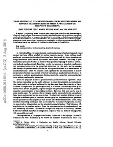
The diffusion problem ● Physical formulation (scheme)
6
Introduction
Parameterizations / Simulation
Comparison
Conclusion
The diffusion problem ● Mathematical formulation
u
c c Kz x z z
c c x, z uc Q z H c Kz 0 z
u u z
x 0, 0 z h at
x0
at
z 0, h
(5)
K z K z x, z
7
Introduction
Parameterizations / Simulation
Comparison
Conclusion
● Parameterization of vertical profiles of turbulent parameters
u ln z / z0 m z / L m z0 / L , z zb u u zb , z zb 2 2 2 3 10 z z u * w2 1.44 w*2 1 0.7 2 9 h h w *
z 0 . 59 , w L Tw 4z 8z h 0.15 h h 1 e 0.0003e , w
(6)
(7)
z 0. 1 h z 0.1 h
(8)
● Input variables for the diffusion problem (turbulent scales)
z0 , L, h, u* 8
Introduction
Parameterizations / Simulation
Comparison
Conclusion
Numerical solution of the diffusion problem
Nz = 200; ∆ x = 0.1 s; 9
Introduction
Parameterizations / Simulation
Comparison
Conclusion
Comparative analysis of the results ● Some details of the Copenhagen diffusion experiment and
numerical simulation Number of experiment
u(115), m s-1
σw(115), m s-1
Date
L, m
h, m
u*, m s-1
measured
modeled
measured
modeled
1
20.09.78
-46
1980
0.37
3.4
3.9
0.83
0.91
2
26.09.78
-384
1920
0.74
10.6
8.6
1.07
1.21
3
19.10.78
-108
1120
0.39
5.0
4.1
0.68
0.77
4
03.11.78
-173
390
0.39
4.6
4.7
0.47
0.66
5
09.11.78
-577
820
0.46
6.7
5.6
0.71
0.70
6
30.04.79
-569
1300
1.07
13.2
12.8
1.33
1.65
7
27.06.79
-136
1850
0.65
7.6
6.9
0.87
1.26
Remark: z0 = 0.6 m
ru = 0.98
rσ = 0.94
10
Introduction
Parameterizations / Simulation
Comparison
Conclusion
Comparison of vertical eddy diffusivities ● Vertical profiles (experiment 3)
11
Introduction
Parameterizations / Simulation
Comparison
Conclusion
Comparison of vertical eddy diffusivities ● Horizontal profiles (experiment 3)
12
Introduction
Parameterizations / Simulation
Comparison
Conclusion
Comparison of concentrations ● Horizontal profiles of concentration at the ground (experiment 3)
13
Introduction
Parameterizations / Simulation
Comparison
Conclusion
Comparison of concentrations ● C – C plot between the observed and the modelled concentrations
14
Introduction
Parameterizations / Simulation
Comparison
Conclusion
● Observed and computed crosswind-integrated concentrations N exper.
Parameters of numerical scheme
C0/Q × 10-4, s m-2
Distance from the source, m
Observed
Nz
Δz, m
Δx, m
1
200
9.8
0.1
1900
1
200
9.8
0.1
2
200
9.5
2
200
3
Modeled Par. (1)
Par. (2)
Par. (3)
Par. (4)
Kz=f(z)
6.48
5.59
4.32
5.27
4.96
3.40
3700
2.31
3.39
1.59
2.84
2.76
2.03
0.1
2100
5.38
2.66
2.84
2.80
3.01
2.21
9.5
0.1
4200
2.95
2.36
1.47
2.09
1.86
1.41
200
5.6
0.1
1900
8.20
5.86
4.52
5.64
5.99
4.40
3
200
5.6
0.1
3700
6.22
4.09
1.90
3.54
3.74
2.87
3
200
5.6
0.1
5400
4.30
2.97
1.25
2.56
2.75
2.23
4
200
1.9
0.1
4000
11.70
5.80
4.20
5.42
6.19
5.19
5
200
4.1
0.1
2100
6.72
4.96
4.38
5.02
5.72
4.37
5
200
4.1
0.1
4200
5.84
4.05
2.03
3.60
4.00
3.07
5
200
4.1
0.1
6100
4.97
3.16
1.44
2.79
3.15
2.48
6
200
6.5
0.1
2000
3.96
1.84
1.97
1.95
2.27
1.70
6
200
6.5
0.1
4200
2.22
1.65
0.95
1.46
1.46
1.11
6
200
6.5
0.1
5900
1.83
1.27
0.59
1.09
1.13
0.88
7
200
9.2
0.1
2000
6.70
3.12
2.90
3.14
3.18
2.27
7
200
9.2
0.1
4100
3.25
2.25
1.17
1.93
1.84
1.37
0.30
0.90
0.37
0.29
0.69
NMSE =/()
15
Introduction
Parameterizations / Simulation
Comparison
Conclusion
Conclusion ● The memory effects in near-source area are very important ● The best parameterization is (4) (Degrazia, 2000): NMSE = 0.29. Complex! ● Simpler parameterizations (1) (Arya, 1995) and (3) (Voloshchuk, 2002) work well: NMSE = 0.30 and 0.37 ● The additional factors (*) and (**) for Kz can easily be used to take memory effects into account
cx (*) cl x
x 1 e l (**)
16