Parameterized Algorithms for Feedback Vertex Set Iyad Kanj1 1
Michael Pelsmajer2
Marcus Schaefer1
School of Computer Science, Telecommunications and Information Systems, DePaul University, 243 S. Wabash Avenue, Chicago, IL 60604-2301. {ikanj,mschaefer}@cs.depaul.edu? 2 Department of Applied Mathematics, Illinois Institute of Technology, Chicago, IL 60616.
[email protected]
Abstract. We present an algorithm for the parameterized feedback vertex set problem that runs in time O((2 lg k + 2 lg lg k + 18)k n2 ). This improves the previous O(max{12k , (4 lg k)k }nω ) algorithm by Raman et al. by roughly a 2k factor (nw ∈ O(n2.376 ) is the time needed to multiply two n × n matrices). Our results are obtained by developing new combinatorial tools and employing results from extremal graph theory. We also show that for several special classes of graphs the feedback vertex set problem can be solved in time ck nO(1) for some constant c. This includes, for example, graphs of genus O(lg n).
1
Introduction
Given an undirected graph G, a feedback vertex set in G is a subset of vertices F in G such that G − F is acyclic. The size of a feedback vertex set F is |F |. The feedback vertex set problem (FVS) is: given a graph G and a positive integer k, decide if G has a feedback vertex set of size at most k. It is well-known that the FVS problem is NP-complete on both directed and undirected graphs [17]. The minimization version of this problem has been studied intensively from the approximability point of view [1, 2, 13, 16, 24] due to its important applications in fields like circuit testing, deadlock resolution, and analyzing manufacturing processes [13, 18, 21]. For example, in the field of circuit testing, a small set of registers (vertices) needs to be identified in the circuit (graph) whose removal makes the circuit testable (i.e., the circuit needs to be acyclic) [18]. The FVS problem has also received considerable attention from the parameterized complexity point of view [3, 4, 10, 11, 23]. A parameterized problem is said to be fixed-parameter tractable if the problem can be solved in time f (k)nO(1) for some function f which is independent of n [11]. The class FPT denotes the class of all fixed-parameter tractable problems [11]. It was shown that the FVS problem on undirected graphs is in FPT [4, 10, 11], whereas it remains an open question whether the FVS problem on directed graphs is in FPT [11]. ?
The first author was supported in part by DePaul University Competitive Research Grant.
Once a problem has been shown to be in FPT, the search for better algorithms for the problem continues; that is, algorithms that remain practical for larger values of the parameter k. Successful examples of such developments include the vertex cover and planar dominating set problems (see [7, 15] and their references). The same holds true for the FVS problem on undirected graphs. Bodlaender [4], and Downey and Fellows [10], were the first to show that the problem is in FPT. In [11], Downey and Fellows presented an O((2k + 1)k n2 ) time algorithm for the problem. Becker et al. [3] gave a randomized algorithm running in time O(4k kn) that finds a minimum feedback vertex set of size k with k probability at least 1 − (1 − 4−k )c4 for an arbitrary constant c. By observing that every undirected graph on n vertices with minimum degree at least 3 has a cycle of length bounded by 2 lg n + 1, Raman presented a very simple algorithm for the problem running in time O((6k lg k)k+1 nω ) [22], where nω ∈ O(n2.376 ) is the running time of the best algorithm for multiplying two n × n matrices [8]. More recently, using some nice combinatorial techniques, Raman et al. [23] presented an algorithm for the problem running in time O(max{12k , (4 lg k)k }nω ) improving significantly the O((2k + 1)k n2 ) time algorithm given in [11] (when k is sufficiently large). In this paper we continue the efforts towards reducing the running time of the algorithms for the FVS problem. We develop new combinatorial tools and employ known results from extremal graph theory to show that the size of a minimum feedback vertex set is Ω(n/ lg n) in a graph with no cycles of length bounded by lg n. This allows us to obtain an O((2 lg k+2 lg lg k + 18)k n2 ) time algorithm for the FVS problem, improving the previous O(max{12k , (4 lg k)k }nω ) time algorithm in [23] by roughly a 2k factor. Obviously, the running time of this algorithm is still far from being practical, and the question of whether the FVS problem can be solved in time ck nO(1) remains open. We also consider the FVS problem on special classes of graphs. We show that the problem on graphs of genus O(lg n) and on K r -minor free graphs is solvable in time ck nO(1) for some constant c. We also show that the problem on bipartite graphs, graphs of genus O(n² ) for any ² > 0, and constant average degree graphs, can be solved in time ck nO(1) for some constant c if and only if the FVS problem on general graphs can.
2
Preliminaries
Let G = (V, E) be an undirected graph. For a set of vertices S in G we denote by G − S the subgraph of G that results from removing the vertices in S, together with all edges incident to them. A minimum feedback vertex set is a feedback vertex set of minimum size. We denote by γ(G) the size of a minimum feedback vertex set in G. For a vertex v, we denote by deg(v) the degree of v in G. Let v be a vertex in G such that deg(v) ≤ 2. We define the following operation, which is standard in the literature. If deg(v) = 1 then remove v (together with its incident edge) from G; if deg(v) = 2 and the two neighbors x and y of v are not adjacent, then remove v and add an edge between x and y. Let us denote
this operation by Short-Cut(v). We say that the operation Short-Cut() is applicable to a vertex v, if either deg(v) = 1, or deg(v) = 2 and the two neighbors of v are non-adjacent. A variation of the following proposition appears in [23] (see [2] for a proof). Proposition 1. (Lemma 1, [23]) Let G be an undirected graph and let v be a vertex in G to which the operation Short-Cut() is applicable. Let G0 be the graph resulting from applying Short-Cut(v). Then γ(G0 ) = γ(G). We assume that we have a subroutine Clean(G) which applies the operation Short-Cut() repeatedly to G until the operation is no longer applicable. It is clear from Proposition 1 that if G0 is the resulting graph from applying Clean(G), then γ(G0 ) = γ(G). The graph G is said to be clean, if Clean(G) is not applicable. Note that any degree-2 vertex in a clean graph must be on a cycle of length three. An almost shortest cycle in G is a cycle whose length is at most the length of a shortest cycle in G plus one. It is well-known that an almost shortest cycle in an undirected graph with n vertices can be found in time O(n2 ) [19]. It is also well-known that any undirected graph with minimum degree at least 3 has a cycle of length at most 2 lg n + 1 [12].
3
The Algorithm
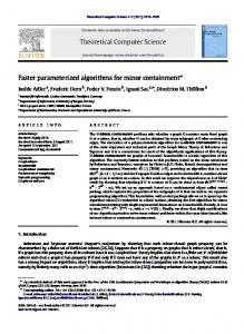
The basic idea behind most of the parameterized algorithms for the FVS problem presented so far has been to branch on short cycles and use the search tree method [11, 22, 23]. Suppose we are trying to determine if there exists a feedback vertex set in G of size bounded by k. Let C be a cycle in G of length l. Then every feedback vertex set of G must contain at least one vertex of C. For every vertex v on C, we can include v in the feedback vertex set, and then recurse to determine if G − v has a feedback vertex set of size k − 1. Let us call such a process: branching on the cycle C. If we let T (k) be the number of nodes in the search tree of such an algorithm that looks for a feedback vertex set of size bounded by k, then when the algorithm branches on a cycle of length l, T (k) can be expressed using the recurrence relation T (k) ≤ l · T (k − 1) + 1. The number of nodes in the search tree corresponding to the algorithm is O((lmax )k ), where lmax is the length of the longest cycle the algorithm branches on [11]. The running time of the algorithm is now proportional to the number of nodes in the search tree multiplied by the time we spend at every node of the search tree to find a cycle and process the graph. Thus, to reduce the running time of the algorithm, it is desirable to branch on short cycles. Most parameterized algorithms so far hinge on this approach [11, 22, 23]. In this section we develop another algorithm that uses this approach (based on the algorithm in [23]). We present the algorithm in Figure 1 below. We prove its correctness and analyze its running time in the next section.
FVS-solver Input: an instance (G, k) of FVS Output: a feedback vertex set F of G of size bounded by k in case it exists 0. 1. 2. 3. 4. 5.
F = ∅; if G is acyclic then return(F ); if k = 0 and G contains a cycle then return(’NO’); apply Clean(G); let C be an almost shortest cycle in G of length l; √ if l > 13 and k ≤ 3 n then return(’NO’); else if l > lg n + 1 and (lg n > lg k + lg lg k + 13) then return(’NO’); else if l > max{2 lg k + 18, 2 lg n − 9} then return(’NO’); else branch on C and update k, F , and G accordingly; Fig. 1. The algorithm FVS-solver
4
Analysis of FVS-solver
The main idea behind the analysis of the algorithm presented in [23] is that if the graph does not contain a cycle of constant length, then the size of the feedback vertex set k must be large. In particular, the following structural result immediately follows from [23]. Lemma 1. (Theorem 2, [23]) Let G be a graph on n vertices with minimum √ degree at least 3. If there is no cycle in G of length at most 12 then γ(G) > 3 n. The above result shows that when a clean graph has no cycle of length bounded by 12 (note that no degree-2 vertex√exists in G at this point since G does not contain a cycle of length 3), k > 3 n, and hence, lg n < 2 lg k − 3. Since every undirected graph with minimum degree at least 3 must have a cycle of length bounded by 2 lg n + 1, G has a cycle of length bounded by 4 lg k. An algorithm that branches on a shortest cycle will then either branch on a cycle of length at most 12, or of length at most 4 lg k. According to the discussion in the previous section, this gives a search tree of size O((max{12, 4 lg k})k ). In this section we develop new combinatorial techniques and employ results from extremal graph theory to improve this analysis. The structural results obtained in this section will allow us to prove an upper bound of O((2 lg k+2 lg lg k+ 18)k ) on the size of the search tree of the algorithm FVS-solver presented in the previous section. Let T be a tree. For a vertex v in T we denote by dT (v) the degree of v in T . A vertex v ∈ T is said to be good if dT (v) ≤ 2. The statement of the following lemma can be easily proved.3 Lemma 2. There are at least bq/2 + 1c good vertices in a tree on q vertices. 3
An easy way to see why the statement is true is to note that the average degree of a tree is bounded by 2.
For a good vertex u in T , {u} is said to be a nice set if dT (u) ≤ 1, and for two good vertices u and v in T , the set {u, v} is said to be a nice set if (u, v) is an edge in T . Lemma 3. Let T be a tree, and let ng be the number of good vertices in T . Then there exists at least b(ng + 1)/2c nice sets in T that are pairwise disjoint. Proof. Without loss of generality, we assume that T is rooted at a vertex r. We define the natural parent-child, and ancestor-descendent relationships, between the vertices in T . Note that each vertex in T is either the root vertex or has exactly one parent in T . For every vertex v in T , let Tv denote the subtree of T rooted at v and containing all its descendents. We will prove the following statement: if Tv contains q good vertices of T , then the number of pairwise disjoint nice sets in Tv is at least b(q + 1)/2c. It is clear that the previous statement will imply the statement of the lemma because T = Tr . (Observe that a good vertex in Tv might not be a good vertex in T , and this is why we require the q vertices to be good in T .) To prove the statement, let Tv be a rooted subtree of T , and proceed by induction on q. Tv must contain at least one leaf of T , so q > 0. If q ≤ 2, then Tv must contain a leaf u in T , and {u} is a nice set. Therefore the number of (pairwise disjoint) nice sets in this case is at least 1 ≥ b(q + 1)/2c. Suppose now that the number of pairwise disjoint nice sets in any rooted tree containing p good vertices from T , for 2 ≤ p < q, is at least b(p + 1)/2c. We distinguish two cases. Case 1. v has at least two children. Let v1 , . . . , vd , be the children of v in Tv . Let qi be the number of good vertices in T that are in Tvi , i = 1 . . . d, and note that 1 ≤ qi < q, and that q ≤ q1 + . . . qd + 1 (v might be good, in which case it is the root of the tree and d = 2). By the inductive hypothesis, each Tvi contains at least b(qi + 1)/2c pairwise disjoint nice sets in T . Since every nice set in Tvi is disjoint from every nice set in Tvj for 1 ≤ i 6= j ≤ d, it follows that Tv contains at least b(q1 + . . . + qd + d)/2c = b(q1 + . . . qd + 1 + d − 1)/2c ≥ b(q + 1)/2c pairwise disjoint nice sets in T (note that d ≥ 2). Case 2. v has exactly one child v 0 . In this case v must be a good vertex in T . If v 0 is good, let v 00 be the child of v 0 in Tv (note that v 00 must exist since q > 2). Now Tv00 contains q − 2 good vertices in T . By induction, the number of pairwise disjoint nice sets in Tv00 is at least b(q − 1)/2c. Since {v, v 0 } is a nice set which is disjoint from all the nice sets in Tv00 , it follows that the number of pairwise disjoint nice sets in Tv is at least b(q + 1)/2c. If v 0 is bad, then v 0 must have at least two children in Tv0 . The proof now is identical to that of Case 1 by applying induction on the trees rooted at the children of v 0 . This completes the induction and the proof.
u t
This lemma follows directly from Lemma 2 and Lemma 3. Lemma 4. Let T be a tree on q vertices. There are at least q/4 pairwise disjoint nice sets in T .
Let (G, k) be an instance of FVS, where G is clean and has n vertices, and assume that G does not have a cycle of length bounded by 12. Since G is clean and has no cycles of length 3, G has minimum degree at least 3. Let F be a minimum feedback set of G, let f = |F |, and F = G − F . Applying Lemma 4 to every tree in F, we get that F (i.e., the trees in F) contains at least (n − f )/4 pairwise disjoint nice sets. So if we let S be the set of pairwise disjoint nice sets in F, then |S| ≥ (n − f )/4. We construct a graph GF as follows. The set of vertices of GF is F . The edges of GF are defined as follows. Let {a, b} be a nice set in S. Since a and b are good in F (i.e., in the tree of F that they belong to) and both have degree greater or equal to 3 in G, a must have at least one neighbor in F , and b must have at least one neighbor F . Pick exactly one neighbor a1 of a in F , and exactly one neighbor b1 of b in F . Note that a1 and b1 must be distinct since G has no cycles of length 3. Add the edge (a1 , b1 ) to GF . Now let {a} be a nice set in S, then a must have at least two neighbors in F . We pick exactly two neighbors a1 and a2 of a in F , and we add the edge (a1 , a2 ) in GF . This completes the construction of GF . Since G has no cycles of length bounded by 6, for any two distinct nice sets in S, the edges associated with them in GF are distinct. This means that GF is a simple graph with at least (n − f )/4 edges. We have the following lemma. Lemma 5. If GF has a cycle of length l then G has a cycle of length bounded by 3l. Proof. Let (v1 , . . . , vl , v1 ) be a cycle in GF . Since each (vi , vi+1 ) (the index arithmetic is taken modulo l) is an edge in GF , (vi , vi+1 ) is associated with a nice set Si in S. If Si = {a}, let Pi be the path (vi , a, vi+1 ) in G; if Si = {a, b}, let Pi be the path (vi , a, b, vi+1 ) in G. Since the nice sets in S are disjoint, the paths Pi , i = 1, . . . , l, are internally vertex-disjoint in G, and they determine a cycle of length bounded by 3l. u t The following result is known in extremal graph theory (see [5, 6, 14]). Lemma 6. Let G be a graph with n vertices where n ≥ 3. If G does not contain a cycle of length at most 2l, then the number of edges in G is bounded by 90ln1+1/l . Theorem 1. Let G be a graph with n ≥ 3 vertices and with no cycles of length bounded by max{12, lg n}. Then γ(G) ≥ (n/(61 lg n))1−6/(lg n+6) . Proof. Suppose that G does not have a cycle of length bounded by max{12, lg n}. Let F be a minimum feedback vertex set of G, and let f = |F | = γ(G). Since G has no cycles of length bounded by 12, if we let F and GF be as defined in the above discussion, then it follows from above that the number of edges in GF is at least (n − f )/4. Since G does not have a cycle of length bounded by lg n, by Lemma 5, GF has no cycle of length bounded by (lg n)/3. Applying Lemma 6 with l = (lg n)/6, we get that the number of edges in GF is bounded by 15(lg n)f 1+6/ lg n . Thus
(n − f )/4 ≤ 15(lg n)f 1+6/ lg n n ≤ 60(lg n)f 1+6/ lg n + f ≤ 60(lg n)f 1+6/ lg n + f 1+6/ lg n n ≤ 61(lg n)f 1+6/ lg n
(1)
Manipulating (1) we get f ≥ (n/(61 lg n))1−6/(lg n+6) completing the proof. u t Theorem 1 implies that the size of a minimum feedback vertex set in a graph with minimum degree at least 3 and no cycles of length bounded by lg n must be Ω(n/ lg n). Corollary 1. Let G be a graph with n ≥ 3 vertices and with no cycles of length bounded by max{12, lg n}. Then lg n ≤ lg γ(G) + lg lg γ(G) + 13. Proof. Applying the lg () function on both sides of (1) in Theorem 1 we get lg n ≤ lg 61 + lg lg n + lg f + 6 lg f / lg n
(2)
Since G has no cycles of length bounded by 12, from Lemma 1 we get lg n < 2 lg f , and hence lg lg n < 1 + lg lg f . Now noting that lg 61 ≤ 6 and lg f ≤ lg n, it follows from (2) that lg n ≤ lg f + lg lg f + 13. u t Lemma 7. Let G be a graph with n vertices and minimum degree at least 3. For any integer constant d > 0, there is a cycle in G of length at most max{2 lg γ(G) + 2 lg (d − 1) + 3, 2 lg n − 2 lg (d + 1) + 4}. Proof. Let d > 0 be given, and let ∆ be the maximum degree of G. By Lemma 4 in [23], γ(G) > (δ − 2)n/(2(∆ − 1)), where δ is the minimum degree of the graph. Since δ ≥ 3, we get n < 2(∆ − 1)γ(G), and hence lg n < lg γ(G) + lg (∆ − 1) + 1 2 lg n + 1 < 2 lg γ(G) + 2 lg (∆ − 1) + 3
(3)
Let r be a vertex in G of degree ∆. Perform a breadth-first search starting at r until a shortest cycle is first encountered in the graph. Let l be the length of the shortest cycle first encountered in this process. Since r has degree ∆ and every other vertex has degree at least 3, it is not difficult to show, using a counting argument, that the number of vertices in the graph is at least ∆(2(l−2)/2 − 1) + 1 if l is even, and ∆(2(l−1)/2 − 1) + 1 if l is odd. Suppose that l ≥ 4. We have n ≥ ∆(2(l−2)/2 − 1) + 1 n > ∆(2(l−2)/2 − 1) lg n > lg ∆ + lg (2(l−2)/2 − 1)
(4)
Also l ≥ 4 implies that 2(l−2)/2 ≥ 2. Using the inequality lg (x − 1) ≥ lg x − 1 for x ≥ 2 in (4), and manipulating (4), we get l ≤ 2 lg n − 2 lg ∆ + 4
(5)
If l < 4, then l = 3 and since n > ∆, (5) is still true. Now if ∆ ≤ d, then from the fact that G has a cycle of length bounded by 2 lg n + 1, and from (3), we conclude that there is a cycle in G of length at most 2 lg γ(G) + 2 lg (∆ − 1) + 3 ≤ 2 lg γ(G) + 2 lg (d − 1) + 3. Otherwise, ∆ ≥ d + 1, and by (5), there is a cycle in G of length at most 2 lg n − 2 lg ∆ + 4 ≤ 2 lg n − 2 lg (d + 1) + 4. It follows that G has a cycle of length at most max{2 lg γ(G) + 2 lg (d − 1) + 3, 2 lg n − 2 lg (d + 1) + 4}. This completes the proof. u t Corollary 2. Let G be a graph with minimum degree at least 3. There exists a cycle in G of length at most max{2 lg γ(G) + 17, 2 lg n − 10} Proof. Apply Lemma 7 with d = 127.
u t
Theorem 2. Let G be a graph with n vertices. In time O((2 lg k+2 lg lg k + 18)k n2 ) we can decide if G has a feedback vertex set of size bounded by k. Proof. It is not difficult to see that the algorithm FVS-solver solves the FVS problem. In particular, √ if FVS-solver returns a NO answer in step 5, then either (i) l > 13 and k ≤ 3 n, or (ii) l > lg n + 1 and lg n > lg k + lg lg k + 13, or (iii) l > max{2 lg k + 18, 2 lg n − 9}. Since l is the length of an almost shortest cycle, if (i) holds then G does not have a cycle of length bounded by 12, and hence no feedback vertex set of size bounded by k by Lemma 1. If (ii) holds, then G does not have a cycle of length bounded by max{12, lg n}, and hence no feedback vertex set of size bounded by k by Corollary 1 (note that in this case n ≥ 3, and l must also be greater than 13 since lg n > 13). Finally if (iii) holds, then G has no cycle of length bounded by {2 lg k + 17, 2 lg n − 10}. From Corollary 2 (note that G has minimum degree at least three at this point since G is clean and has no cycles of length three) we conclude that k must be smaller than γ(G), and hence G has no feedback vertex set of size bounded by k. To analyze the running time of the algorithm, let l be the length of a cycle C that the algorithm branches on. By looking at step 5 in the algorithm, we see that if the algorithm branches√on C then one of the following cases must hold: (a) l ≤ 13, or (b) l > 13, k > 3 n, and l ≤ lg n + 1, or (c) lg n ≤ lg k + lg lg k + 13 and l ≤ max{2 lg k + 18, 2 lg n − 9}. If (b) holds, then the conditions in (b) give that l < 2 lg k. If (c) holds, then combining the two inequalities in (c) we get l ≤ max{2 lg k + 18, 2 lg k + 2 lg lg k + 17} ≤ 2 lg k + 2 lg lg k + 18. It follows that in all cases (a), (b), and (c), the algorithm branches on a cycle of length at most 2 lg k + 2 lg lg k + 18.
Thus, according to the discussion at the beginning of this section, the size of the search tree corresponding to the algorithm is O((2 lg k + 2 lg lg k + 18)k ). Now at each node of the search tree the algorithm might need to find an almost shortest cycle, call Clean(), check if the graph is acyclic, and process the graph. Finding an almost shortest cycle takes O(n2 ) time. When Clean() is applied, since every vertex that Clean() removes has degree bounded by 2, Clean() can be implemented to run in linear time in the number of vertices it removes, and hence, in O(n) time. Checking if the graph is acyclic and processing the graph takes no more than O(n2 ) time. It follows that the running time of the algorithm is O((2 lg k + 2 lg lg k + 18)k n2 ). u t According to the above theorem, the algorithm FVS-solver improves the algorithm in [23] by roughly a 2k factor.
5
FVS On Special Classes of Graphs
In this section we consider the FVS problem on special classes of graphs. We look at the following classes: bipartite graphs, bounded genus graphs, and K r -minor free graphs for fixed r. Bipartite Graphs Let G be a graph with n vertices and m edges. Consider the operation of subdividing an edge e in G by introducing a degree-2 vertex v. Then this operation is precisely the inverse operation of Short-Cut(v). Therefore, if we let G0 be the graph obtained from G by subdividing an edge e ∈ G, then it follows from Proposition 1 that γ(G0 ) = γ(G). Subdividing each edge in G yields a bipartite graph G0 , which according to the previous statement satisfies γ(G0 ) = γ(G). The graph G0 has n + m vertices and 2m edges. This shows that the FVS problem on general graphs can be solved in time f (k)nO(1) if and only if the FVS problem on bipartite graphs can be solved in f (k)nO(1) time. In particular, an algorithm of running time ck nO(1) (for some constant c) for the FVS problem on bipartite graph implies an algorithm of running time ck nO(1) for the FVS problem on general graphs. Bounded Genus Graphs The following lemma follows from a standard Euler-formula argument. Lemma 8. Let G be a graph with n vertices, minimum degree at least 3, and genus g. If n ≥ 8g then there is a cycle in G of length at most 12. Let G be a graph with n0 vertices and genus g0 satisfying g0 ≤ c lg n0 for some constant c. Note that if we branch on a cycle in G or process G as in the algorithm FVS-solver, the number of vertices and genus of G change, and the relationship g ≤ c lg n, where n and g are the number of vertices and genus, respectively, in the
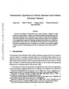
resulting graph may not hold. However, since the operations in FVS-solver do not increase the genus of the graph, the genus g of the resulting graph satisfies g ≤ g0 ≤ c lg n0 . Consider the algorithm BGFVS-solver given in Figure 2, which is a modification of the algorithm FVS-solver presented in Section 1, that will solve the FVS problem on graphs of genus bounded by c lg n. BGFVS-solver Input: an instance (G, k) of FVS where G has n0 vertices and genus g0 Output: a feedback vertex set F of G of size bounded by k in case it exists and g0 satisfies g0 ≤ c lg n0 0. 1. 2. 3. 4. 5. 6.
F = ∅; if G is acyclic then return(F ); if k = 0 and G contains a cycle then return (’NO’); apply Clean(G); if the number of vertices n of G is bounded by 8c lg n0 then solve the problem by brute force and STOP; let C be an almost shortest cycle in G of length l; if l > 13 then return(’Invalid Instance’); else branch on C and update k, F , and G accordingly; Fig. 2. The algorithm BGFVS-solver
It is not difficult to see the correctness of the algorithm BGFVS-solver. The only step that needs clarification is when the algorithm returns in step 6 that the instance is invalid. If this happens, then the number of vertices n in the resulting graph G must satisfy n > 8c lg n0 , where n0 is the number of vertices in the original graph, and G does not have a cycle of length bounded by 12 (note that the algorithm finds an almost shortest cycle). Since the genus of the resulting graph g is bounded by the genus g0 of the original graph, if g0 satisfies the condition g0 ≤ c lg n0 then we would have 8g ≤ 8g0 ≤ 8c lg n0 ≤ n, which according to Lemma 8, would imply the existence of a cycle of length at most 12 in G (since G has minimum degree at least 3 at this point). Since no such cycle exists in G, the genus g0 in the original graph does not satisfy the condition g0 ≤ c lg n0 , and hence the input instance does not satisfy the genus bound requirement. Therefore the algorithm rejects the instance in this case. This shows actually that BGFVS-solver does not need to know in advance if the input instance satisfies the genus bound requirement or not. As long as the input instance satisfies the genus bound requirement, the algorithm solves the problem. Now to analyze the running time of the algorithm, we note that step 4 can be carried out in time O(n8c+1 ) by enumerating every subset of vertices in the 0 graph and checking whether it is a feedback vertex set of size bounded by k. The algorithm never branches on a cycle of length greater than 13. It follows that the running time of the algorithm is O(13k n8c+ω+1 ). 0
Theorem 3. The FVS problem on graphs of genus O(lg n) can be solved in time 13k nO(1) . Let G be a graph with n0 vertices and genus g0 , and let ² > 0 be given. We 2/² construct a graph G0 as follows. Let W be a wheel on n0 vertices. Add W to G by linking a vertex in W other than the center to any vertex in G. It is easy to verify that γ(G0 ) = γ(G) + 2, and that a feedback vertex set of G can be constructed from a feedback vertex set of G0 easily. Since a wheel is planar, it follows that the genus g 0 of G is equal to g. The number of vertices n0 of G0 is 2/² n0 = n0 + n0 . Therefore g 0 = g ≤ n20 ≤ n0² . This shows that we can reduce the FVS problem on general graphs to the FVS problem on graphs of genus O(n² ) (for any ² > 0) in polynomial time such that if the FVS problem on graphs of genus O(n² ) can be solved in f (k)nO(1) time, then so can the FVS problem on general graphs. In particular, if the FVS problem on graphs of genus O(n² ) can be solved in time ck nO(1) then so can the FVS problem on general graphs.4 K r -Minor Free Graphs Let r be a constant, and let Gr be the class of graphs with minimum degree at least 3 and no K r -minor. Combining theorems from [20, 25] and [26] as described in [9, p180], we have the following: There exists √ a constant c such that, for all r, each G ∈ Gr has a cycle of length less than cr lg r. Let G be a K r -minor free graph with minimum degree at least 3. According to√the result described above, there is a cycle in G of length bounded by c1 = cr lg r, which is a constant. Therefore, if we modify the algorithm FVS-solver so that it branches on an almost shortest cycle after applying Clean(G), then the algorithm always branches on a cycle of length at most c0 = 1 + max{3, c1 }.5 This shows that the running time of the modified algorithm is O(c0k n2 ). Theorem 4. For any constant r, the FVS problem on K r -minor free graphs can be solved in time O(c0k n2 ), where c0 is a constant.
References 1. V. Bafna, P. Berman, and T. Fujito. A 2-approximation algorithm for the Undirected Feedback Vertex Set problem. SIAM Journal on Discrete Mathematics, 12(3):289–297, 1999. 2. Reuven Bar-Yehuda, Dan Geiger, Joseph Naor, and Ron M. Roth. Approximation algorithms for the feedback vertex set problem with applications to constraint satisfaction and bayesian inference. SIAM Journal on Computing, 27(4):942–959, 1998. 4
5
Using the same technique, one can prove that if the FVS problem on graphs with average degree bounded by a constant, can be solved in time f (k)nO(1) , then so can the FVS problem on general graphs. Note that if the length of the almost shortest cycle that the algorithm computes is not bounded by c0 , the algorithm rejects the instance.
3. A. Becker, R. Bar-Yehuda, and D. Geiger. Random algorithms for the Loop Cutset problem. Journal of Artificial Intelligence Research, 12:219–234, 2000. 4. H. Bodlaender. On disjoint cycles. International Journal of Foundations of Computer Science, 5:59–68, 1994. as. Extremal Graph Theory. Academic Press, London, 1978. 5. B. Bollob´ 6. J. A. Bondy and M. Simonovits. Cycles of even length in a graph. J. Combinatorial Theory (B), 16:97–105, 1974. 7. J. Chen, I. Kanj, and W. Jia. Vertex cover: further observations and further improvements. Journal of Algorithms, 41:280–301, 2001. 8. D. Coppersmith and S. Winograd. Matrix multiplication via arithmetic progression. Journal of Symbolic Computation, 9:251–280, 1990. 9. R. Diestel. Graph Theory (2nd Edition). Springer-Verlag, New York, 2000. 10. R. Downey and M. Fellows. Fixed-parameter tractability and completeness. Congressus Numerantium, 87:161–187, 1992. 11. R. Downey and M. Fellows. Parameterized Complexity. Springer, New York, 1999. 12. P. Erdos and L. Posa. On the maximal number of disjoint circuits of a graph. Pubbl. Math. Debrecen, 9:3–12, 1962. 13. G. Even, J. Naor, B. Schieber, and M. Sudan. Approximating minimum feedback sets and multicuts in directed graphs. Algorithmica, 20(2):151–174, 1998. 14. R. J. Faudree and M. Simonovits. On a class of degenerate extremal graph problems. Combinatorica, 3 (1):83–93, 1983. 15. F. Fomin and D. Thilikos. Dominating sets in planar graphs: branch-width and exponential speed-up. In Proceedings of the 14th ACM-SIAM Symposium on Discrete Algorithms, pages 168–177, 2003. 16. T. Fujito. A note on approximation of the Vertex Cover and Feedback Vertex Set problems-unified approach. Information Processing Letters, 59(2):59–63, 1996. 17. M. Garey and D. Johnson. Computers and Intractability: A Guide to the Theory of NP-Completeness. W. H. Freeman, New York, 1979. 18. R. Gupta, R. Gupta, and M. Breuer. Ballast: A methodology for partial scan design. IEEE Transactions on Computers, 39(4):538–544, 1990. 19. A. Itai and M. Rodeh. Finding a minimum circuit in a graph. SIAM Journal on Computing, 7(4):413–423, 1978. 20. A. V. Kostochka. The minimum Hadwiger number for graphs with a given mean degree of vertices. Metody Diskret. Analiz., 38:37–58, March 1982. 21. A. Kunzmann and H. Wunderlich. An analytical approach to the partial scan problem. Journal of Electronic Testing: Theory and Applications, 1:163–174, 1990. 22. V. Raman. Parameterized complexity. In Proceedings of the 7th National Seminar on Theoretical Computer Science, pages 1–18, 1997. 23. V. Raman, S. Saurabh, and C. Subramanian. Faster fixed-parameter tractable algorithms for Undirected Feedback Vertex Set. In Proceedings of the 13th Annual International Symposium on Algorithms and Computation, volume 2518 of Lecture Notes in Computer Science, pages 241–248, 2002. 24. P. Seymour. Packing directed circuits fractionally. Combinatorica, 15(2):281–288, 1995. 25. A. Thomason. An extremal function for contractions of graphs. Math. Proc. Cambridge Philos. Soc., 95(2):261–265, 2001. 26. C. Thomassen. Girth in graphs. J. Combin. Theory Ser. B, 35:129–141, March 1983.