PHYSICAL REVIEW E 76, 041906 共2007兲
Parameters of stochastic diffusion processes estimated from observations of first-hitting times: Application to the leaky integrate-and-fire neuronal model Susanne Ditlevsen* Department of Biostatistics, University of Copenhagen, Øster Farimagsgade 5, 1014 Copenhagen K, Denmark
Petr Lansky† Institute of Physiology, Academy of Sciences of the Czech Republic, Videnska 1082, 142 20 Prague 4, Czech Republic 共Received 17 January 2007; published 9 October 2007兲 A theoretical model has to stand the test against the real world to be of any practical use. The first step is to identify parameters in the model estimated from experimental data. In many applications where renewal point data are available, models of first-hitting times of underlying diffusion processes arise. Despite the seemingly simplicity of the model, the problem of how to estimate parameters of the underlying stochastic process has resisted solution. The few attempts have either been unreliable, difficult to implement, or only valid in subsets of the relevant parameter space. Here we present an estimation method that overcomes these difficulties, is computationally easy and fast to implement, and also works surprisingly well on small data sets. The method is illustrated on simulated and experimental data. Two common neuronal models—the Ornstein-Uhlenbeck and Feller models—are investigated. DOI: 10.1103/PhysRevE.76.041906
PACS number共s兲: 87.19.La, 02.50.⫺r, 05.40.⫺a
The first-hitting time to a constant threshold of a diffusion process has been in focus for stochastic modeling of problems where a hidden random process only shows when it reaches a certain level that triggers some observable event. Applications come from various fields: e.g., biology, survival analysis, mathematical finance, and others. The application in this paper originates from neuronal modeling. Neurons transfer information by emitting electrical pulses 共spikes兲, and diffusion models describe the underlying dynamics of the interspike intervals 共ISIs兲. They represent the time evolution of the neuronal membrane depolarization, modeled by a scalar process Xt given by an Itô stochastic differential equation dXt = 共Xt, 兲dt + 共Xt, 兲dW共t兲,
X0 = x0 ,
共1兲
where and are real-valued functions 共the infinitesimal drift and variance兲, is a p-dimensional parameter, and W共t兲 is a standard Wiener process 共Brownian motion兲. An alternative description to Eq. 共1兲 is the Fokker-Planck equation for the transition density f 共x , t 兩 x0 , 0兲 关1兴. Firing of spikes is not an intrinsic part of model 共1兲, so a firing threshold has to be imposed. A firing event occurs when the membrane voltage Xt exceeds a voltage threshold for the first time, here assumed to be a constant S ⬎ x0. After a spike, the membrane depolarization is reset to the initial value. Formally, the ISIs are identified with the first-passage time 共hitting time兲 of Xt across S, T = inf兵t 艌 0: Xt 艌 S兩X0 = x0 ⬍ S其.
共2兲
Thus, we assume the ISIs form a renewal process—i.e., that they are independent and identically distributed. The properties of the random variable T including its probability density
function g共t 兩 x0 , S兲 = g共t兲 have been extensively studied. The distribution g共t兲 is only known for a few simple models, and approximation techniques have been devised 关2兴, of which many are based on the renewal equation, the so-called Fortet’s equation 关3,4兴 relating the first-passage-time density and the transition density f 共·兲 for x 艌 S, f 共x,t兩x0,0兲 =
冕
t
f 共x,t兩S, 兲g共兩x0,S兲d .
共3兲
0
We write F共x , t − s 兩 xs兲 = 兰x f 共u , t 兩 xs , s兲du for the corresponding transition distribution function. Estimation of has been extensively studied; see e.g., 关5–8兴, or 关9–11兴 in the neuronal context. All these methods are based on complete or partial observations of the trajectory of X共t兲. However, if only first-passage times are available, attempts to solve the estimation problem are rare; some references are 关12–14兴. We proposed Laplace-transform moment estimators for two specific diffusion models 关15,16兴; see also the cited papers therein. These estimators have certain drawbacks: e.g., they are only valid in a subspace of the parameter space 关17兴 and the variance parameter is poorly determined. Recently we proposed a method based on an integral equation applicable to any one-dimensional diffusion process with known transition density 关18兴, which we will apply in this paper. Parameter estimation. Consider the sample t1 , . . . , tn of n independent observations of T from which will be estimated. The method applies the integral equation 共3兲 as described in the following; see also 关18兴. The probability P关Xt ⬎ S兩X0 = x0兴 = 1 − F共S,t兩x0兲
共4兲
*
[email protected]; URL: http://staff.pubhealth.ku.dk/⬃sudi/ †
[email protected]
1539-3755/2007/76共4兲/041906共5兲
can alternatively be calculated by the transition integral 041906-1
©2007 The American Physical Society
PHYSICAL REVIEW E 76, 041906 共2007兲
SUSANNE DITLEVSEN AND PETR LANSKY
P关Xt ⬎ S兩X0 = x0兴 =
冕
t
g共u兲关1 − F共S,t − u兩S兲兴du.
t s= ,
共5兲
0
For fixed , Eq. 共4兲 is a function of t and can be calculated directly. The value of Eq. 共5兲 can be estimated at t from the sample by the average n
1 兺 关1 − F共S,t − ti兩S兲兴1兵ti艋t其 , n i=1
共6兲
where 1A is the indicator function of the set A, since it is the expected value of 1T苸关0,t兴关1 − F共S,t − T兩S兲兴,
共7兲
with respect to the distribution of T for fixed . A statistical error measure is then defined as the maximum over t of the distance between 共4兲 and 共6兲, suitably normalized by dividing by 共兲 = supt⬎0关1 − F共S , t 兩 x0兲兴 so that 共4兲 will vary between 0 and 1 for all . To find the maximum over t a grid on the positive real line has to be chosen. A good choice for fixed is the set 兵t 苸 R+ : 关1 − F共S , t 兩 x0兲兴 / 共兲 = i / N , i = 1 , . . . , N − 1其 for some reasonably large number N. In the applications below N = 100. The estimator of is finally obtained by minimizing this error function over the parameter space. The estimate is denoted ˆ . Ornstein-Uhlenbeck neuronal model. A phenomenological way to introduce stochasticity into the deterministic leakyintegrator model dx共t兲 / dt = −x共t兲 / + is by assuming an additional term of Gaussian white noise. This model is a special case of model 共1兲 for which
共x兲 = −
x + ,
共x兲 = ⬎ 0,
x0 = 0,
共8兲
where ⬎ 0 is the membrane time constant and and are constants characterizing neuronal input. Model 共8兲 is the Ornstein-Uhlenbeck 共OU兲 process 关1,15,19–22兴. The transition density function is Gaussian, f 共x,t兲 = 共2Vt兲−1/2 exp兵− 共x − M t兲2/共2Vt兲其, −t/
共9兲
−2t/
兲 / 2. Despite where M t = 共1 − e 兲 and Vt = 共1 − e many efforts, an analytical solution for the first-passage-time density has only been found for S = 关20,23,24兴. Two types of parameters appear: the intrinsic parameters and the parameters characterizing the input 关25兴. The intrinsic parameters are constants given prior to the verification of the model: the firing threshold S, the initial depolarization x0, and the membrane time constant reflecting spontaneous voltage decay in absence of input. The input parameters are related to the signal coded by the neuron: characterizes the depolarization of the membrane between spikes, and characterizes the random variability in the depolarization process. It is convenient to reformulate models 共1兲 and 共8兲 to the equivalent dimensionless form 2
dY s = 共− Y s + ␣兲ds + dWs, where
Y 0 = 0,
共10兲
Ys =
Xt , S
Ws =
Wt
冑
␣=
,
, S
=
冑 , S 共11兲
and T / = inf兵s ⬎ 0 : Y s 艌 1其. It shows that only two parameters are identifiable from ISI data, in contrast to when sample trajectories of the process are available. Therefore, without loss of generality, all considerations in the following will be related to the dimensionless process Y s and its first crossing of the level 1. Note, however, that the model now operates on the time scale of s = t / , not on the original measured time scale. All observed ISIs thus have to be transformed by dividing by . The membrane time constant has to be assumed or otherwise estimated from other types of data. Increasing ␣ results in shorter ISIs. Increasing  when ␣ ⬎ 1 increases the ISI variability, whereas in the subthreshold regime 关26兴 showed that the coefficient of variation was nonmonotone as a function of the noise level. Let ⌽共·兲 be the normal cumulative distribution function. Combining 共4兲 and 共9兲 we obtain P关Y s ⬎ 1兩Y 0 = 0兴 = ⌽
冉冑
␣共1 − e−s兲 − 1
1 − e−2s/冑2
冊
,
共12兲
which we estimate from the sample using 共6兲 by n
冉 冑
1 ␣−1 ⌽ 兺 n i=1  / 冑2
冊
1 − e−共s−si兲 1兵si艋s其 , 1 + e−共s−si兲
共13兲
where si = ti / . The normalizing constant is given by ⌽关共␣ − 1兲 / 共 / 冑2兲兴 for ␣ 艌 0 and ⌽关−冑1 − 2␣ / 共 / 冑2兲兴 for ␣ ⬍ 0. Then ␣ˆ and ˆ can be transformed to physically interpretable quantities of and through 共11兲. Simulated data. Trajectories of the OU process were simulated according to the Euler scheme for four different combinations of parameter values: 共␣ , 兲 = 共0.8, 1兲, 共1,0.1兲, 共2,0.1兲, and 共2,1兲, respectively. The process was run until the trajectory reached the threshold where the time was recorded. We generated 1000 samples with 10 observations each for each combination of parameter values. This was repeated for sample sizes of 50, 100, and 500, respectively. On all samples ␣ and  were estimated; estimation results are summarized in Fig. 1, where the densities of the estimates for different sample sizes are plotted. The estimators behave well even for sample sizes of only 50 observations. Thus, we expect the method to be reliable if the data are well described by the OU model. As appears from Fig. 1, the estimators seem asymptotically well described by a normal distribution, which can be used to construct confidence intervals. In Table I mean and standard deviations of the samples of 1000 estimates are reported for all combinations of parameter values and sample sizes. A reasonable confidence interval would then be the estimate ±2 times the standard deviation. As would be expected, the standard deviation of the estimator seems approximately proportional to  and inversely proportional to the square root of the sample size. Auditory thalamic neurons in guinea pigs. The first two sets of experimental ISI data were recorded intracellularly from the auditory system of a guinea pig 共for details of the
041906-2
PHYSICAL REVIEW E 76, 041906 共2007兲
PARAMETERS OF STOCHASTIC DIFFUSION PROCESSES…
C
D
1.0 ^ α
1.1
F
0
50
50
E
0.9
1.9
2.0 ^ α
2.1
1
G
2 ^ α
3
1.0 ^ β
1.5
H 7
1.3
80
0.8 ^ α
0.5
1.0 ^ β
1.5
0.05
0.10 ^ β
0.15 0.05
0
0
0
0
Densities
7
0.3
0
0
0
Densities
50
5
B
5
A
0.10 ^ β
0.15
0.5
FIG. 1. Densities of estimates for simulated data based on 1000 estimates. Upper panels: estimates of ␣. Lower panels: estimates of . Solid black lines: sample sizes of 500. Dashed black lines: sample sizes of 100. Solid gray lines: sample sizes of 50. Dashed gray lines: sample sizes of 10. Vertical lines: true values used in the simulations: 共A兲, 共E兲 共␣ , 兲 = 共0.8, 1兲; 共B兲, 共F兲 共␣ , 兲 = 共1 , 0.1兲; 共C兲, 共G兲 共␣ , 兲 = 共2 , 0.1兲; 共D兲, 共H兲 共␣ , 兲 = 共2 , 1兲. Note different scales.
stimulation protocol, data acquisition, and processing see 关27兴兲. The first set contains ISIs during the spontaneous activity, and being based on the intracellular data 共not only the ISIs兲, the parameters were also estimated by standard procedures 关10兴. This permits us to evaluate the new estimation procedure. Moreover, intracellular data gives “exact” information about the threshold value, the reset value, and the membrane time constant. The second set, obtained from the same neuron, contains the first ISIs within the stimulation TABLE I. Summary of estimates from data simulated from model 共10兲. The last two columns are sample mean± sample standard deviation 共SSD兲 of estimates. Parameter value 共␣ , 兲 共0.8, 1兲 共0.8, 1兲 共0.8, 1兲 共0.8, 1兲 共1, 0.1兲 共1, 0.1兲 共1, 0.1兲 共1, 0.1兲 共2, 0.1兲 共2, 0.1兲 共2, 0.1兲 共2, 0.1兲 共2, 1兲 共2, 1兲 共2, 1兲 共2, 1兲
Sample size
Estimates of ␣ mean± SSD
Estimates of  mean± SSD
10 50 100 500 10 50 100 500 10 50 100 500 10 50 100 500
1.086± 0.276 0.881± 0.164 0.838± 0.127 0.796± 0.061 1.011± 0.084 1.000± 0.016 0.999± 0.012 0.998± 0.005 1.992± 0.043 1.996± 0.018 1.996± 0.013 1.996± 0.006 2.035± 0.441 1.978± 0.206 1.973± 0.151 1.965± 0.065
0.759± 0.255 0.910± 0.141 0.943± 0.107 0.975± 0.046 0.027± 0.034 0.097± 0.018 0.099± 0.013 0.100± 0.006 0.097± 0.039 0.097± 0.012 0.098± 0.009 0.099± 0.004 0.899± 0.268 0.953± 0.129 0.967± 0.090 0.977± 0.040
period. The intrinsic parameters were considered to be the same as for the spontaneous activity. The spontaneous record consists of 312 ISIs. In 关10兴 the intrinsic parameters were estimated to S − x0 = 11 mV and = 39 ms. Transforming the observed ISIs by dividing by this , the dimensionless parameters were estimated to ␣ˆ = 0.852 and ˆ = 0.094. Using 共11兲 we obtain the following estimates ˆ = 0.240 V / s and ˆ = 0.005 V / 冑s. for the input parameters: In 关10兴 the median values for these were 0.285 V / s for with most estimates falling in the range 0.1– 0.45 V / s, and 0.014 V / 冑s for with most estimates falling in the range 0.01– 0.016 V / 冑s. Note that since we base the estimation on the hitting times, we obtain only one set of estimates for the entire record, whereas in 关10兴 the estimation is based on intracellular observations and different sets of estimates for the input parameters are obtained for each ISI. Both parameters estimated only with the information contained in the hitting times were of the same order of magnitude as the estimations using all the information in the data set. A mean parameter is easier to estimate than a variance parameter, and accordingly appears precisely determined judged by the estimation from the intercellular recording. The stimulated record consists of 83 ISIs. Using the intrinsic parameters estimated from the spontaneous part, we ˆ = 1.351 V / s estimated ␣ˆ = 4.79 and ˆ = 0.625, obtaining and ˆ = 0.035 V / 冑s. Note that the value of , which reflects intensity of stimulation, is 5-6 times larger than for the spontaneous activity. To check the adequacy of the OU model with the estimated parameter values for these data, Eq. 共12兲 and the empirical equation 共13兲 are compared in Fig. 2, after dividing by ⌽关共␣ˆ − 1兲 / 共ˆ / 冑2兲兴. Especially the stimulated record shows a good fit. Feller neuronal model. In many applications the OU process is unrealistic because it is unbounded. Introducing an
041906-3
PHYSICAL REVIEW E 76, 041906 共2007兲
SUSANNE DITLEVSEN AND PETR LANSKY
B 0.01 0.02 ISIs (s)
−0.007 0.208
−0.108– 0.212 0.085–0.722
OU model, all 24 olfactory neurons. Feller model, 18 olfactory neurons. c Units: 关V / 冑s兴 共OU兲, 关冑V / s兴 共Feller兲.
0 ⬍ y 0 ⬍ 1, 共15兲
2共␣/兲 艌 1, 2
1.0
was available, and we could find no values in the literature for this specific type of neurons. In 关33兴 共p. 56兲 the values of the membrane time constant are given as ranging from 10 to 50 ms. We assume that sensory neurons, despite different modalities, have similar membrane time constants, and we therefore used the values from the previous application of 39 ms. There were 24 data records containing between 27 and 1907 ISIs in each record. Both the OU model and the Feller model were fitted. Summaries are given in Table II.
0.5
共14兲
where 2 艌 2. In dimensionless form it becomes dY s = 共− Y s + ␣兲ds + 共/冑␣兲冑Y sdWs,
−0.059– 0.218 0.017–0.078
A 1 ISIs (s)
B
0.0
共x兲 = 冑x − VI ,
0.030 0.041
1.0
inhibitory reversal potential VI ⬍ x0 ⬍ S leads to model 共1兲 with x + ,
Rangeb
b
FIG. 2. Auditory neurons. Comparison of the 共normalized兲 right-hand side of Eq. 共12兲 共solid curves兲 to the 共normalized兲 empirical equation 共13兲 共dashed curves兲, calculated with estimated parameters. Vertical axes can be interpreted as a cumulative probability; horizontal axes are ISIs 共s兲. 共A兲 Spontaneous record: ␣ˆ = 0.85, ˆ = 0.09. 共B兲 Stimulated record: ␣ˆ = 4.8, ˆ = 0.63. Note different time axes.
共x兲 = −
Medianb
0.5
ISIs (s)
Rangea
a
Cumulative Probability
Cumulative probability
4
ˆ 关V/s兴 ˆ c
Mediana
0.0
0
A 2
0
Cumulative probability 1
1
TABLE II. Summary of estimates from olfactory neurons for S − x0 = 11 mV, = 39 ms, and x0 − VI = 11 mV.
2
1 ISIs (s)
2
where Y s = 共Xt − VI兲/共S − VI兲,
C
␣ = 共 − VI兲/共S − VI兲,
0
5
10 15 time (s)
=
冕
1.0 0.5
1.0
D 2 ISIs (s)
s
f共u兲兵1 − F2关a共s − u兲, , ␦共s − u,1兲兴其du, 共16兲
0
The normalizing constant is given by 共1 − F2关4␣/2, ,0兴兲. Spontaneous firing of olfactory receptor neurons in rats. The next sets of ISIs were obtained during spontaneous activity of normally breathing and tracheotomized rats 共for details see 关31,32兴兲. No information on intrinsic parameters
4
2 ISIs (s)
4
F
with a共s兲 = 4␣ / 关2共1 − e−s兲兴, degrees of freedom = 4共␣ / 兲2, and noncentrality parameter
␦共s,y 0兲 = 共4␣y 0/2兲关e−s/共1 − e−s兲兴.
E
0.0
1 − F2关a共s兲, , ␦共s,y 0兲兴
0.5
Model 共15兲 is known as the Feller process 关16,28,29兴, or the CIR process in mathematical finance 关30兴. The transition density follows a noncentral 2 distribution F2关·兴 关30兴. The integral equation becomes
0.0
 = 冑冑 − VI/共S − VI兲.
Cumulative Probability
and
20
0
20
40 time (s)
60
FIG. 3. Olfactory neurons. 共A兲, 共B兲, 共C兲 Neuron that fits the models. 共D兲, 共E兲, 共F兲 Neuron that did not fit the models. 共A兲, 共D兲 OU model, normalized comparison of the right-hand side of Eq. 共12兲 共solid lines兲 to the empirical equation 共13兲 共dashed lines兲, calculated with estimated parameters. Vertical axes can be interpreted as a cumulative probability; horizontal axes are ISIs 共s兲. 共B兲, 共E兲 Likewise for the Feller model. 共C兲, 共F兲 Corresponding spike trains consisting of 100 spikes. Note different time axes.
041906-4
PHYSICAL REVIEW E 76, 041906 共2007兲
PARAMETERS OF STOCHASTIC DIFFUSION PROCESSES…
Some neurons showed an acceptable fit to both models, and some did not fit at all; see Fig. 3 for examples. For six neurons the Feller model could not be fitted. The ISIs do not contain enough information to distinguish between the two models, and the choice of model has to be based on physical reasons or other types of data: e.g., intracellular recordings. To appreciate the qualitatively different behavior of the neurons that fit and did not fit, respectively, in the lower part of Fig. 3 are typical patterns of activity 共spike trains兲 pictured for the same two neurons. Only the first 100 spikes of the records are plotted, such that both time series contain the same number of spikes. Typically, the neurons that did not fit had a tendency to clustering of spikes with bursts and relatively long periods of silence. The bursting type of activity of these neurons was already mentioned in 关31兴. When neurons show bursting behavior, the assumption of independent and identically distributed ISIs is obviously violated. In this case
more elaborate models taking account of the autocorrelation should be considered. Moreover, neither the OU nor Feller model can produce this combination of many short ISIs with a heavy tail of long ISIs in the distribution. In conclusion, we have presented a method to compare stochastic diffusion models with experimental data of firsthitting times, providing seemingly good estimators for physical quantities previously considered very difficult to obtain. Also a diagnostic tool for model evaluation is provided. The authors thank P. Ducham-Viret, M. Chaput, and J.F. He for making their experimental data available. This work was supported by grants from the Danish Medical Research Council and the Lundbeck Foundation to S.D. and the Center for Neurosciences LC554, AV0Z50110509 and Academy of Sciences of the Czech Republic 共Information Society, 1ET400110401兲 to P.L.
关1兴 C. Gardiner, Handbook of Stochastic Methods for Physics, Chemistry and the Natural Sciences 共Springer, Berlin, 1983兲. 关2兴 L. Ricciardi, A. Di Crescenzo, V. Giorno, and A. Nobile, Math. Japonica 50, 247 共1999兲. 关3兴 J. Durbin, J. Appl. Probab. 8, 431 共1971兲. 关4兴 R. Fortet, J. Math. Pures Appl. 22, 177 共1943兲. 关5兴 B. Bibby and M. Sørensen, Bernoulli 1, 17 共1995兲. 关6兴 Y. Kutoyants, Statistical Inference for Ergodic Diffusion Processes, Springer Series in Statistics 共Springer, New York, 2003兲. 关7兴 B. Prakasa Rao, Statistical Inference for Diffusion Type Processes 共Oxford University Press, New York, 1999兲. 关8兴 H. Sørensen, Int. Statist. Rev. 72, 337 共2004兲. 关9兴 P. Lansky, Math. Biosci. 67, 247 共1983兲. 关10兴 P. Lansky, P. Sanda, and J. He, J. Comput. Neurosci. 21, 211 共2006兲. 关11兴 R. Höpfner, Math. Biosci. 207共2兲, 275 共2007兲. 关12兴 J. Inoue, S. Sato, and L. Ricciardi, Biol. Cybern. 73, 209 共1995兲. 关13兴 S. Shinomoto, Y. Sakai, and S. Funahashi, Neural Comput. 11, 935 共1999兲. 关14兴 L. Paninski, J. Pillow, and E. Simoncelli, Neural Comput. 16, 2533 共2004兲. 关15兴 S. Ditlevsen and P. Lansky, Phys. Rev. E 71, 011907 共2005兲. 关16兴 S. Ditlevsen and P. Lansky, Phys. Rev. E 73, 061910 共2006兲. 关17兴 S. Ditlevsen, Statistics & Probability Letters 共to be published兲. 关18兴 S. Ditlevsen and O. Ditlevsen, in Parameter Estimation from Observations of First-Passage Times of the OrnstienUhlenbeck Process and the Feller Process, special issue of Probabilistic Engineering Mechanics 共to be published兲.
关19兴 W. Gerstner and W. Kistler, Spiking Neuron Models 共Cambridge University Press, Cambridge, England, 2002兲. 关20兴 L. Ricciardi, Diffusion Processes and Related Topics in Biology 共Springer, Berlin, 1977兲. 关21兴 H. Tuckwell, Nonlinear and Stochastic Theories, Introduction to Theoretical Neurobiology, Vol. 2 共Cambridge University Press, Cambridge, England, 1988兲. 关22兴 L. Ricciardi and L. Sacerdote, Biol. Cybern. 35, 1 共1979兲. 关23兴 A. R. Bulsara, T. C. Elston, C. R. Doering, S. B. Lowen, and K. Lindenberg, Phys. Rev. E 53, 3958 共1996兲. 关24兴 L. Alili, P. Patie, and J. Pedersen, Stoch. Models 21, 967 共2005兲. 关25兴 H. Tuckwell and W. Richter, J. Theor. Biol. 71, 167 共1978兲. 关26兴 K. Pakdaman, S. Tanabe, and T. Shimokawa, Neural Networks 14, 895 共2001兲. 关27兴 Y. Yu, Y. Xiong, Y. Chan, and J. He, J. Neurosci. 24, 3060 共2004兲. 关28兴 W. Feller, in Diffusion Processes in Genetics, Proceedings of the Second Berkeley Symposium on Mathematical Statistics and Probability, edited by J. Neyman 共University of California Press, Berkeley, 1951兲, pp. 227–246. 关29兴 P. Lansky, L. Sacerdote, and F. Tomasetti, Biol. Cybern. 73, 457 共1995兲. 关30兴 J. Cox, J. Ingersoll, and S. Ross, Econometrica 53, 385 共1985兲. 关31兴 P. Duchamp-Viret, L. Kostal, M. Chaput, P. Lansky, and J. Rospars, J. Neurobiol. 65, 97 共2005兲. 关32兴 L. Kostal and P. Lansky, Biol. Cybern. 94, 157 共2006兲. 关33兴 Fundamentals of Neurophysiology, edited by R. Schmidt 共Springer, New York, 1978兲.
041906-5