Apr 22, 2010 - checkVarsQQ generates a QQ plot of the quantiles of gene specific sample variances against the quantiles of the scaled inverse chi-square ...
Parametric Empirical Bayes Methods for Microarrays Ming Yuan, Ping Wang, Deepayan Sarkar, Michael Newton and Christina Kendziorski April 22, 2010
Contents 1 Introduction
1
2 General Model Structure: Two Conditions
2
3 Multiple Conditions
3
4 The 4.1 4.2 4.3
4 4 4 5
Three Models The Gamma Gamma Model . . . . . . . . . . . . . . . . . . . . . . . . . The Lognormal Normal Model . . . . . . . . . . . . . . . . . . . . . . . . The Lognormal Normal with Modified Variance Model . . . . . . . . . .
5 EBarrays
5
6 Case Study
7
7 Appendix: Comparison with the older versions of EBarrays
15
8 References
27
1
Introduction
We have developed an empirical Bayes methodology for gene expression data to account for replicate arrays, multiple conditions, and a range of modeling assumptions. The methodology is implemented in the R package EBarrays. Functions calculate posterior probabilities of patterns of differential expression across multiple conditions. Model assumptions can be checked. This vignette provides a brief overview of the methodology and its implementation. For details on the methodology, see Newton et al. 2001, Kendziorski et al., 2003, and Newton and Kendziorski, 2003. We note that some of the function calls in version 1.7 of EBarrays have changed. 1
2
General Model Structure: Two Conditions
Our models attempt to characterize the probability distribution of expression measurements xj = (xj1 , xj2 , . . . , xjI ) taken on a gene j. As we clarify below, the parametric specifications that we adopt allow either that these xji are recorded on the original measurement scale or that they have been log-transformed. Additional assumptions can be considered within this framework. A baseline hypothesis might be that the I samples are exchangeable (i.e., that potentially distinguishing factors, such as cell-growth conditions, have no bearing on the distribution of measured expression levels). We would thus view measurements xji as independent random deviations from a gene-specific mean value µj and, more specifically, as arising from an observation distribution fobs (·|µj ). When comparing expression samples between two groups (e.g., cell types), the sample set {1, 2, . . . , I} is partitioned into two subsets, say s1 and s2 ; sc contains the indices for samples in group c. The distribution of measured expression may not be affected by this grouping, in which case our baseline hypothesis above holds and we say that there is equivalent expression, EEj , for gene j. Alternatively, there is differential expression (DEj ) in which case our formulation requires that there now be two different means, µj1 and µj2 , corresponding to measurements in s1 and s2 , respectively. We assume that the gene effects arise independently and identically from a system-specific distribution π(µ). This allows for information sharing amongst genes. Were we instead to treat the µj ’s as fixed effects, there would be no information sharing and potentially a loss in efficiency. Let p denote the fraction of genes that are differentially expressed (DE); then 1 − p denotes the fraction of genes equivalently expressed (EE). An EE gene j presents data xj = (xj1 , . . . , xjI ) according to a distribution ! Z Y I f0 (xj ) = fobs (xji |µ) π(µ) dµ. (1) i=1
Alternatively, if gene j is DE, the data xj = (xj1 , xj2 ) are governed by the distribution f1 (xj ) = f0 (xj1 ) f0 (xj2 )
(2)
owing to the fact that different mean values govern the different subsets xj1 and xj2 of samples. The marginal distribution of the data becomes pf1 (xj ) + (1 − p)f0 (xj ).
(3)
With estimates of p, f0 , and f1 , the posterior probability of differential expression is calculated by Bayes’ rule as p f1 (xj ) . p f1 (xj ) + (1 − p) f0 (xj )
(4)
To review, the distribution of data involves an observation component, a component describing variation of mean expression µj , and a discrete mixing parameter p governing 2
the proportion of genes differentially expressed between conditions. The first two pieces combine to form a key predictive distribution f0 (·) (see (1)), which enters both the marginal distribution of data (3) and the posterior probability of differential expression (4).
3
Multiple Conditions
Many studies take measurements from more than two conditions, and this leads us to consider more patterns of mean expression than simply DE and EE. For example, with three conditions, there are five possible patterns among the means, including equivalent expression across the three conditions (1 pattern), altered expression in just one condition (3 patterns), and distinct expression in each condition (1 pattern). We view a pattern of expression for a gene j as a grouping or clustering of conditions so that the mean level µj is the same for all conditions grouped together. With microarrays from four cell conditions, there are 15 different patterns, in principle, but with extra information we might reduce the number of patterns to be considered. We discuss an application in Section 6 with four conditions, but the context tells us to look only at a particular subset of four patterns. We always entertain the null pattern of equivalent expression among all conditions. Consider m additional patterns so that m + 1 distinct patterns of expression are possible for a data vector xj = (xj1 , . . . , xjI ) on some gene j. Generalizing (3), xj is governed by a mixture of the form m X pk fk (xj ), (5) k=0
where {pk } are mixing proportions and component densities {fk } give the predictive distribution of measurements for each pattern of expression. Consequently, the posterior probability of expression pattern k is P (k|xj ) ∝ pk fk (xj ).
(6)
The pattern-specific predictive density fk (xj ) may be reduced to a product of f0 (·), contributions from the different groups of conditions, just as in (2); this suggests that the multiple-condition problem is really no more difficult computationally than the twocondition problem except that there are more unknown mixing proportions pk . Furthermore, it is this reduction that easily allows additional parametric assumptions to be considered within the EBarrays framework. In particular, three forms for f0 are currently specified (see section 4), but other assumptions can be considered simply by providing alternative forms for f0 . The posterior probabilities (6) summarize our inference about expression patterns at each gene. They can be used to identify genes with altered expression in at least one condition, to order genes within conditions, to classify genes into distinct expression patterns and to estimate FDR. 3
4
The Three Models
We consider three particular specifications of the general mixture model described above. Each is determined by the choice of observation component and mean component, and each depends on a few additional parameters θ to be estimated from the data. As we will demonstrate, the model assumptions can be checked using diagnostic tools implemented in EBarrays, and additional models can be easily implemented.
4.1
The Gamma Gamma Model
In the Gamma-Gamma (GG) model, the observation component is a Gamma distribution having shape parameter α > 0 and a mean value µj ; thus, with scale parameter λj = α/µj , λαj xα−1 exp{−λj x} fobs (x|µj ) = Γ(α) for measurements x > 0. Note that the coefficient of variation (CV) in this distribution √ is 1/ α, taken to be constant across genes j. Matched to this observation component is a marginal distribution π(µj ), which we take to be an inverse Gamma. More specifically, fixing α, the quantity λj = α/µj has a Gamma distribution with shape parameter α0 and scale parameter ν. Thus, three parameters are involved, θ = (α, α0 , ν), and, upon integration, the key density f0 (·) has the form �α−1 �Q I x i i=1 f0 (x1 , x2 , . . . , xI ) = K � (7) �Iα+α0 , PI ν + i=1 xi where ν α0 Γ(Iα + α0 ) K= . ΓI (α) Γ(α0 )
4.2
The Lognormal Normal Model
In the lognormal normal (LNN) model, the gene-specific mean µj is a mean for the log-transformed measurements, which are presumed to have a normal distribution with common variance σ 2 . Like the GG model, LNN also demonstrates a constant CV: p exp(σ 2 ) − 1 on the raw scale. A conjugate prior for the µj is normal with some underlying mean µ0 and variance τ02 . Integrating as in (1), the density f0 (·) for an n-dimensional input becomes Gaussian with mean vector µ0 = (µ0 , µ0 , . . . , µ0 )t and exchangeable covariance matrix � � Σn = σ 2 In + τ0 2 Mn , where In is an n × n identity matrix and Mn is an n × n matrix of ones. 4
4.3
The Lognormal Normal with Modified Variance Model
In the lognormal normal with modified variance (LNNMV) model, the log-transformed measurements are presumed to have a normal distribution with gene-specific mean µj and gene-specific variance σj2 . With the same prior for the µj as in the LNN model, the density f0 (·) for an n-dimensional input from gene j becomes Gaussian with mean vector µ0 = (µ0 , µ0 , . . . , µ0 )t and exchangeable covariance matrix � � Σn = σj2 In + τ0 2 Mn , Thus, only two model parameters are involved once the σj2 ’s are estimated. In the special case of two conditions, we illustrate how to estimate the σj2 ’s. We assume that the prior distribution of σj2 is the scaled inverse chi-square distribution with ν0 degrees of freedom and scale parameter σ0 and that µj1 and µj2 , the gene-specific means in condition 1 and 2, are known. Then the posterior distribution of σj2 is also the scaled inverse chi-square distribution with n1 + n2 + ν0 degrees of freedom and scale parameter s P 2 P 1 (yji − µj2 )2 (xji − µj1 )2 + ni=1 ν0 σ02 + ni=1 , n 1 + n 2 + ν0 where xji is the log-transformed measurement in condition 1, j indexes gene, i indexes sample; yji is the log-transformed measurement in condition 2; n1 , n2 are the numbers of samples in condition 1, 2 respectively. By viewing the pooled sample variances Pn1 P 2 ¯j )2 + ni=1 (yji − y¯j )2 2 i=1 (xji − x σ ˜j = n1 + n2 − 2 ν0 , σ ˆ02 ), the estimate as a random sample from the prior distribution of σj2 , we can get (ˆ 2 2 of (ν0 , σ0 ) using the method of moments [5]. Then our estimate of σj is P 1 P 2 νˆ0 σ ˆ02 + ni=1 (xji − x¯j )2 + ni=1 (yji − y¯j )2 2 σ ˆj = , n1 + n2 + νˆ0 − 2 2 the posterior ν0 , σ02 , µj1 and µj2 substituted by νˆ0 , σ ˆ02 , x¯j and y¯j , where Pn1 mean of σj with P n2 1 1 x¯j = n1 i=1 xji and y¯j = n2 i=1 yji . The GG, LNN and LNNMV models characterize fluctuations in array data using a small number of parameters. The GG and LNN models both involve the assumption of a constant CV. The appropriateness of this assumption can be checked. The LNNMV model relaxes this assumption, allowing for a gene specific variance estimate. Our studies show little loss in efficiency with the LNNMV model, and we therefore generally recommend its use over GG or LNN.
5
EBarrays
The EBarrays package can be loaded by 5
> library(EBarrays) The main user visible functions available in EBarrays are: ebPatterns emfit postprob crit.fun checkCCV checkModel
generates expression patterns fits the EB model using an EM algorithm generates posterior probabilities for expression patterns find posterior probability threshold to control FDR diagnostic plot to check for constant coefficient of variation generates diagnostic plots to check Gamma or Log-Normal assumption on observation component plotMarginal generates predictive marginal distribution from fitted model and compares with estimated marginal (kernel) density of the data; available for the GG and LNN models The form of the parametric model is specified as an argument to emfit, which can be an object of formal class“ebarraysFamily”. These objects are built into EBarrays for the GG, LNN and LNNMV models described above. It is possible to create new instances, using the description given in help(”ebarraysFamily-class”). The data can be supplied either as a matrix, or as an “ExpressionSet” object. It is expected that the data be normalized intensity values, with rows representing genes and columns representing chips. Furthermore, the data must be on the raw scale (not on a logarithmic scale). All rows that contain at least one negative value are omitted from the analysis. The columns of the data matrix are assumed to be grouped into a few experimental conditions. The columns (arrays) within a group are assumed to be replicates obtained under the same experimental conditions, and thus to have the same mean expression level across arrays for each gene. This information is usually contained in the “phenoData” from an “ExpressionSet” object. As an example, consider a hypothetical dataset with I = 10 arrays taken from two conditions — five arrays in each condition ordered so that the first five columns contain data from the first condition. In this case, the phenodata can be represented as 1 1 1 1 1 2 2 2 2 2 and there are two, possibly distinct, levels of expression for each gene and two potential patterns or hypotheses concerning its expression levels: µj1 = µj2 and µj1 6= µj2 . These patterns can be denoted by 1 1 1 1 1 1 1 1 1 1 1 1 1 1 1 2 2 2 2 2 6
representing, in this simple case, equivalent and differential expression for a gene respectively. The choice of admissible patterns is critical in defining the model we try to fit. EBarrays has a function ebPatterns that can read pattern definitions from an external file or a character vector that supplies this information in the above notation. For example, > pattern pattern Collection of 2 patterns Pattern 1 has 1 group Group 1: 1 2 3 4 5 6 7 8 9 10 Pattern 2 has 2 groups Group 1: 1 2 3 4 5 Group 2: 6 7 8 9 10 As discussed below, such patterns can be more complicated in general. For experiments with more than two groups, there can be many more patterns. Zeros can be used in this notation to identify arrays that are not used in model fitting or analysis, as we demonstrate below.
6
Case Study
In collaboration with Dr. M.N. Gould’s laboratory in Madison, we have been investigating gene expression patterns of mammary epithelial cells in a rat model of breast cancer. EBarrays contains part of a dataset from this study (5000 genes in 4 biological conditions; 10 arrays total) to illustrate the mixture model calculations. For details on the full data set and analysis, see Kendziorski et al. (2003). The data can be read in by > data(gould) The experimental information on this data are as follows: in column order, there is one sample in condition 1, two samples in condition 2, five samples in condition 3, and two samples in condition 4: 1 2 2 3 3 3 3 3 4 4 Before we proceed with the analysis, we need to tell EBarrays what patterns of expression will be considered in the analysis. Recall that 15 patterns are possible. Let us first ignore conditions 3 and 4 and compare conditions 1 and 2. There are two possible expression patterns (µCond1 = µCond2 and µCond1 6= µCond2 ). This information can be entered as character strings, or they could also be read from a patternfile which contains the following lines: 7
1 1 1 0 0 0 0 0 0 0 1 2 2 0 0 0 0 0 0 0 A zero column indicates that the data in that condition are not considered in the analysis. The patterns are entered as > pattern pattern Collection of 2 patterns Pattern 1 has 1 group Group 1: 1 2 3 Pattern 2 has 2 groups Group 1: 1 Group 2: 2 3 An alternative approach would be to define a new data matrix containing intensities from conditions 1 and 2 only and define the associated patterns. 1 1 1 1 2 2 This may be useful in some cases, but in general we recommend importing the full data matrix and defining the pattern matrix as a 2 × 10 matrix with the last seven columns set to zero. Doing so facilitates comparisons of results among different analyses since certain attributes of the data, such as the number of genes that are positive across each condition, do not change. The function emfit can be used to fit the GG, LNN or LNNMV model. Posterior probabilities can then be obtained using postprob. The approach is illustrated below. Output is shown for 10 iterations. > gg.em.out gg.em.out EB model fit Family: GG ( Gamma-Gamma ) Model parameter estimates:
8
alpha alpha0 nu Cluster 1 13.26269 1.107481 43.72966 Estimated mixing proportions: Pattern.1 Pattern.2 Cluster 1 0.9970199 0.002980101 > gg.post.out gg.threshold gg.threshold [1] 0.943202 > sum(gg.post.out[, 2] > gg.threshold) [1] 3 > lnn.em.out lnn.em.out EB model fit Family: LNN ( Lognormal-Normal ) Model parameter estimates: mu_0 sigma.2 tao_0.2 Cluster 1 6.733204 0.08110462 1.136083 Estimated mixing proportions: Pattern.1 Pattern.2 Cluster 1 0.9933189 0.006681117 > lnn.post.out lnn.threshold lnn.threshold [1] 0.7707577 > sum(lnn.post.out[, 2] > lnn.threshold) 9
[1] 12 > lnnmv.em.out lnnmv.em.out EB model fit Family: LNNMV ( Lognormal-Normal with modified variances ) Model parameter estimates: mu_0 tao_0.2 1 6.735102 1.131062 Estimated mixing proportions: Pattern.1 Pattern.2 p.temp 0.9929931 0.007006875 > lnnmv.post.out lnnmv.threshold lnnmv.threshold [1] 0.791913 > sum(lnnmv.post.out[, 2] > lnnmv.threshold) [1] 14 > sum(gg.post.out[, 2] > gg.threshold & + lnn.post.out[, 2] > lnn.threshold) [1] 3 > sum(gg.post.out[, 2] > gg.threshold & + lnnmv.post.out[, 2] > lnnmv.threshold) [1] 2 > sum(lnn.post.out[, 2] > lnn.threshold & + lnnmv.post.out[, 2] > lnnmv.threshold) 10
[1] 7 > sum(gg.post.out[, 2] > gg.threshold & + lnn.post.out[, 2] > lnn.threshold & + lnnmv.post.out[, 2] > lnnmv.threshold) [1] 2 The posterior probabilities can be used as described in Newton et al. (2004) to create a list of genes with a target FDR. Using 0.05 as the target FDR, 3, 12 and 14 genes are identified as most likely DE via the GG model, the LNN model and the LNNMV model, respectively. Note that all 3 DE genes identified by the GG model are also identified by LNN; 2 genes are identified as DE by both GG and LNNMV; 7 genes are identified as DE by both LNN and LNNMV; and all three methods agrees on 2 genes being DE. Further diagnostics are required to investigate model fit and to consider the genes identified as DE by only one or 2 models. When using the GG or LNN model, the function checkCCV can be used to see if there is any relationship between the mean expression level and the CV. Another way to assess the goodness of the parametric model is to look at Gamma or Normal QQ plots for subsets of the data sharing common empirical mean intensities. For this, we can choose a small number of locations for the mean value, and look at the QQ plots for the subset of measured intensities in a small window around each of those locations. Since the LNNMV model assumes a log-normal observation component, this diagnostic is suggested when using LNNMV model as well. A third diagnostic consists of plotting the marginal distributions of each model and comparing with the empirical distribution to further assess model fit. This diagnostic is designed especially for the GG and LNN models since their marginal distributions are not gene specific. Finally, checkVarsQQ and checkVarsMar are two diagnostics used to check the assumption of a scaled inverse chi-square prior on σj2 , made in the LNNMV model. checkVarsQQ generates a QQ plot of the quantiles of gene specific sample variances against the quantiles of the scaled inverse chi-square distribution with parameters estimated from data. checkVarsMar plots the density histogram of gene specific sample variances and the density of the scaled inverse chi-square distribution with parameters estimated from the data. Figure 1 shows that the assumption of a constant coefficient of variation is reasonable for the small data set considered here. If necessary, the data could be transformed based on this cv plot prior to analysis. Figure 2 shows a second diagnostic plot for nine subsets of nb = 50 genes spanning the range of mean expression. Shown are qq plots against the best-fitting Gamma distribution. The fit is reasonable here. Note that we only expect these qq plots to hold for equivalently expressed genes, so some violation is expected in general. Figures 3 and 4 show the same diagnostics for the LNN model and the LNNMV model, respectively. A visual comparison between figure 5 and figure 6 suggests that 11
the LNN model provides a better fit. Finally, figure 7 and figure 8 provide checks for the assumption of a scaled inverse chi-square prior on gene specific variances. The LNN model seems most appropriate here. Figure 8 demonstrates that the assumptions of LNNMV are not satisfied, perhaps due to the small sample size (n = 3) used to estimate each gene specific variance. A nice feature of EBarrays is that comparisons among more than two groups can be carried out simply by changing the pattern matrix. For the four conditions, there are 15 possible expression patterns; however, for this case study, four were of most interest. The null pattern (pattern 1) consists of equivalent expression across the four conditions. The three other patterns allow for differential expression. Differential expression in condition 1 only is specified in pattern 2; DE in condition 4 only is specified in pattern 4. The pattern matrix for the four group analysis is now given by 1 1 1 1
1 2 2 1
1 2 2 1
1 2 1 1
1 2 1 1
1 2 1 1
1 2 1 1
1 2 1 1
1 2 2 2
1 2 2 2
> pattern4 pattern4 Collection of 4 patterns Pattern 1 has 1 group Group 1: 1 2 3 4 5 6 7 8 9 10 Pattern 2 has 2 groups Group 1: 1 Group 2: 2 3 4 5 6 7 8 9 10 Pattern 3 has 2 groups Group 1: 1 4 5 6 7 8 Group 2: 2 3 9 10 Pattern 4 has 2 groups Group 1: 1 2 3 4 5 6 7 8 Group 2: 9 10 emfit and postprob are called as before. 12
> gg4.em.out gg4.em.out EB model fit Family: GG ( Gamma-Gamma ) Model parameter estimates: alpha alpha0 nu Cluster 1 17.89911 1.077009 30.36874 Estimated mixing proportions: Pattern.1 Pattern.2 Pattern.3 Cluster 1 0.9780804 0.01864805 0.002403049 Pattern.4 Cluster 1 0.0008684683 > gg4.post.out gg4.threshold2 sum(gg4.post.out[, 2] > gg4.threshold2) [1] 40 > lnn4.em.out lnn4.em.out EB model fit Family: LNN ( Lognormal-Normal ) Model parameter estimates: mu_0 sigma.2 tao_0.2 Cluster 1 6.72002 0.06051488 1.162321 Estimated mixing proportions: Pattern.1 Pattern.2 Pattern.3 Cluster 1 0.9747794 0.02044394 0.003031844 Pattern.4 Cluster 1 0.001744809 13
> lnn4.post.out lnn4.threshold2 sum(lnn4.post.out[, 2] > lnn4.threshold2) [1] 45 > lnnmv4.em.out lnnmv4.em.out EB model fit Family: LNNMV ( Lognormal-Normal with modified variances ) Model parameter estimates: mu_0 tao_0.2 1 6.72525 1.146925 Estimated mixing proportions: Pattern.1 Pattern.2 Pattern.3 p.temp 0.9619806 0.03731805 0.0001265074 Pattern.4 p.temp 0.0005748572 > lnnmv4.post.out lnnmv4.threshold2 sum(lnnmv4.post.out[, 2] > lnnmv4.threshold2) [1] 76 > sum(gg4.post.out[, 2] > gg4.threshold2 & + lnn4.post.out[, 2] > lnn4.threshold2) [1] 34 > sum(gg4.post.out[, 2] > gg4.threshold2 & + lnnmv4.post.out[, 2] > lnnmv4.threshold2) 14
[1] 25 > sum(lnn4.post.out[, 2] > lnn4.threshold2 & + lnnmv4.post.out[, 2] > lnnmv4.threshold2) [1] 29 > sum(gg4.post.out[, 2] > gg4.threshold2 & + lnn4.post.out[, 2] > lnn4.threshold2 & + lnnmv4.post.out[, 2] > lnnmv4.threshold2) [1] 22 The component pattern from postprob is now a matrix with number of rows equal to the number of genes and number of columns equal to 4 (one for each pattern considered). A brief look at the output matrices shows that 40 genes are identified as being in pattern 2 using 0.05 as the target FDR under the GG model, 45 under the LNN model and 76 under the LNNMV model; 34 of the 40 genes identified by GG are also identified by LNN. 25 genes are commonly identified by GG and LNNMV. 29 genes are commonly identified by LNN and LNNMV. 22 genes are identified by all the three models. Figures 9 and 10 show marginal plots similar to Figures 5 and 6. Figure 11 shows a plot similar to figure 8. Here the violation of assumptions made in the LNNMV model is not as severe.
7
Appendix: Comparison with the older versions of EBarrays
Major changes in this version include: 1. A new model LNNMV has been added, as described here. 2. Ordered patterns can be considered. Instead of only considering µj1 6= µj2 , µj1 > µj2 and µj1 < µj2 can also be considered in the current version. For details, please refer to the help page for ebPatterns and Yuan and Kendziorski (2006). 3. Both clustering and DE identification can be done simultaneously by specifying the number of clusters in emfit. For details, please refer to the help page for emfit and Yuan and Kendziorski (2006).
15
0.050 0.002
0.010
CV
0.200
1.000
> checkCCV(gould[, 1:3])
50
100
200
500
1000
2000
5000 10000
Mean
Figure 1: Coefficient of variation (CV) as a function of the mean.
16
> print(checkModel(gould, gg.em.out, model = "gamma", + nb = 50)) mean.ranks
mean.ranks
mean.ranks
3000
2000
5000
140
2000
1500
● ● ●●●● ● ● ● ● ● ● ● ● ● ● ● ● ● ● ● ● ● ● ● ● ● ● ● ● ● ● ● ● ● ● ● ● ● ● ● ● ● ● ● ● ● ● ● ● ● ● ● ● ● ● ● ● ● ● ● ● ● ● ● ● ● ● ● ● ● ● ● ● ● ●
500 1000 1500 2000
600
●● ●●● ● ● ● ● ● ● ● ● ● ● ● ● ● ● ● ● ● ● ● ● ● ● ● ● ● ● ● ● ● ● ● ● ● ● ● ● ● ● ● ● ● ● ● ● ● ● ● ● ● ● ● ● ● ● ● ● ● ● ● ● ● ● ● ● ● ● ● ●● ●
mean.ranks ●
400
250
350
mean.ranks
150
●● ● ●●● ● ● ● ● ● ● ● ● ● ● ● ● ● ● ● ● ● ● ● ● ● ● ● ● ● ● ● ● ● ● ● ● ● ● ● ● ● ● ● ● ● ● ● ● ● ● ● ● ● ● ● ● ● ● ● ● ● ● ● ● ● ● ● ● ● ● ● ● ● ● ● ● ● ●
1000
100 200 300 400
● ● ● ●●● ● ● ● ● ● ● ● ● ● ● ● ● ● ● ● ● ● ● ● ● ● ● ● ● ● ● ● ● ● ● ● ● ● ● ● ● ● ● ● ● ● ● ● ● ● ● ● ● ● ● ● ● ● ● ● ● ● ● ● ● ● ● ● ● ● ● ● ●● ●
200
Quantiles of fitted Gamma distribution
Figure 2: Gamma qq plot.
17
10000 15000
mean.ranks
● ● ● ●● ● ● ● ● ● ● ● ● ● ● ● ● ● ● ● ● ● ● ● ● ● ● ● ● ● ● ● ● ● ● ● ● ● ● ● ● ● ● ● ● ● ● ● ● ● ● ● ● ● ● ● ● ● ● ● ● ● ● ● ● ● ● ● ● ● ● ● ● ● ●● ●
500
mean.ranks 50 100 150
6000
500 1000
800 1200 400
600 1000 200
● ● ●● ● ● ● ● ● ● ● ● ● ● ● ● ● ● ● ● ● ● ● ● ● ● ● ● ● ● ● ● ● ● ● ● ● ● ● ● ● ● ● ● ● ● ● ● ● ● ● ● ● ● ● ● ● ● ● ● ● ● ● ● ● ● ● ● ● ● ● ● ● ●● ●
400 600 800 1000
0
Expression
4000
●● ● ●●● ● ● ● ● ● ● ● ● ● ● ● ● ● ● ● ● ● ● ● ● ● ● ● ● ● ● ● ● ● ● ● ● ● ● ● ● ● ● ● ● ● ● ● ● ● ● ● ● ● ● ● ● ● ● ● ● ● ● ● ● ● ● ● ● ● ● ● ● ●●●
mean.ranks ●
40 60 80 100
●● ●●● ● ● ● ● ● ● ● ● ● ● ● ● ● ● ● ● ● ● ● ● ● ● ● ● ● ● ● ● ● ● ● ● ● ● ● ● ● ● ● ● ● ● ● ● ● ● ● ● ● ● ● ● ● ● ● ● ● ● ● ● ● ● ● ● ● ● ● ● ● ● ●
200
2000
mean.ranks
4000 8000 12000
●●●● ● ● ● ● ● ● ● ● ● ● ● ● ● ● ● ● ● ● ● ● ● ● ● ● ● ● ● ● ● ● ● ● ● ● ● ● ● ● ● ● ● ● ● ● ● ● ● ● ● ● ● ● ● ● ● ● ● ● ● ● ● ● ● ● ● ● ● ● ●●
1000
●
1000 3000 5000
1000
2000
● ●
400
600
> print(checkModel(gould, lnn.em.out, model = "lognormal", + nb = 50))
0.5
−0.5
●
●
0.5
●
0.5
0.0
0.0
●
● ●
−0.5
0.0
0.5
mean.ranks ●
●● ● ● ● ● ● ● ● ● ● ● ● ● ● ● ● ● ● ● ● ● ● ● ● ● ● ● ● ● ● ● ● ● ● ● ● ● ● ● ● ● ● ● ● ● ● ● ● ● ● ● ● ● ● ● ● ● ● ● ● ● ● ● ● ● ● ● ● ● ● ● ● ● ● ●
0.5
0.5
0.5
●● ●● ● ● ● ● ● ● ● ● ● ● ● ● ● ● ● ● ● ● ● ● ● ● ● ● ● ● ● ● ● ● ● ● ● ● ● ● ● ● ● ● ● ● ● ● ● ● ● ● ● ● ● ● ● ● ● ● ● ● ● ● ● ● ● ● ● ● ● ● ● ● ●
0.0
●
0.0
●
●
−0.5
0.0
0.5
Quantiles of Normal N(0,0.081)
Figure 3: Normal qq plot.
18
●
mean.ranks
0.5
● ●● ● ● ● ● ● ● ● ● ● ● ● ● ● ● ● ● ● ● ● ● ● ● ● ● ● ● ● ● ● ● ● ● ● ● ● ● ● ● ● ● ● ● ● ● ● ● ● ● ● ● ● ● ● ● ● ● ● ● ● ● ● ● ● ● ● ● ● ● ● ● ● ●●
0.0
●
−0.5
1
−0.5
mean.ranks
● ●● ● ● ● ● ● ● ● ● ● ● ● ● ● ● ● ● ● ● ● ● ● ● ● ● ● ● ● ● ● ● ● ● ● ● ● ● ● ● ● ● ● ● ● ● ● ● ● ● ● ● ● ● ● ● ● ● ● ● ● ● ● ● ● ● ● ● ● ● ● ● ● ●●●
0.0
●● ● ● ● ● ● ● ● ● ● ● ● ● ● ● ● ● ● ● ● ● ● ● ● ● ● ● ● ● ● ● ● ● ● ● ● ● ● ● ● ● ● ● ● ● ● ● ● ● ● ● ● ● ● ● ● ● ● ● ● ● ● ● ● ● ● ● ● ● ● ● ● ● ● ● ●
−0.5
mean.ranks
−0.5
0.5
−0.5
●
−0.6 −0.2 0.2
0.5 −0.5
0.0
●●● ● ● ● ● ● ● ● ● ● ● ● ● ● ● ● ● ● ● ● ● ● ● ● ● ● ● ● ● ● ● ● ● ● ● ● ● ● ● ● ● ● ● ● ● ● ● ● ● ● ● ● ● ● ● ● ● ● ● ● ● ● ● ● ● ● ● ● ● ● ● ● ● ●
0.0
0.0
mean.ranks
0.5
0.5
mean.ranks
−0.5
−0.5
−0.5 0.0 ●
●● ● ● ● ● ● ● ● ● ● ● ● ● ● ● ● ● ● ● ● ● ● ● ● ● ● ● ● ● ● ● ● ● ● ● ● ● ● ● ● ● ● ● ● ● ● ● ● ● ● ● ● ● ● ● ● ● ● ● ● ● ● ● ● ● ● ● ● ● ● ● ● ● ● ●●●
0.0
0.0
●●● ● ● ● ● ● ● ● ● ● ● ● ● ● ● ● ● ● ● ● ● ● ● ● ● ● ● ● ● ● ● ● ● ● ● ● ● ● ● ● ● ● ● ● ● ● ● ● ● ● ● ● ● ● ● ● ● ● ● ● ● ● ● ● ● ● ● ● ● ● ● ● ●●
−0.5
−0.5
mean.ranks ●
0.5
mean.ranks
●● ●● ● ● ● ● ● ● ● ● ● ● ● ● ● ● ● ● ● ● ● ● ● ● ● ● ● ● ● ● ● ● ● ● ● ● ● ● ● ● ● ● ● ● ● ● ● ● ● ● ● ● ● ● ● ● ● ● ● ● ● ● ● ● ● ● ● ● ● ● ● ● ● ● ● ●●
−2 −1 0
log Expression centered at 0
−0.6 −0.2 0.2
mean.ranks
−0.5
0.0
0.5
> print(checkModel(gould, lnnmv.em.out, + model = "lnnmv", nb = 50, groupid = c(1, + 2, 2, 0, 0, 0, 0, 0, 0, 0)))
−2 −1 0
−2 −1 0
1
2
5
2
0 −2 −1
●
1
●
0
1 0 −1.5 −0.5 0.5
●
2
1
●
2
Quantiles of Standard Normal
Figure 4: Normal qq plot.
19
●
2
1
●
2
mean.ranks
●●● ● ● ● ● ● ● ● ● ● ● ● ● ● ● ● ● ● ● ● ● ● ● ● ● ● ● ● ● ● ● ● ● ● ● ● ● ● ● ● ● ● ● ● ● ● ● ● ● ● ● ● ● ● ● ● ● ● ● ● ● ● ● ● ● ● ● ● ● ● ● ● ●● ● ●
−2 −1 0
1
●●● ● ● ● ● ● ● ● ● ● ● ● ● ● ● ● ● ● ● ● ● ● ● ● ● ● ● ● ● ● ● ● ● ● ● ● ● ● ● ● ● ● ● ● ● ● ● ● ● ● ● ● ● ● ● ● ● ● ● ● ● ● ● ● ● ● ● ● ● ● ● ● ● ● ● ●●
−2 −1 0
mean.ranks
● ●● ● ● ● ● ● ● ● ● ● ● ● ● ● ● ● ● ● ● ● ● ● ● ● ● ● ● ● ● ● ● ● ● ● ● ● ● ● ● ● ● ● ● ● ● ● ● ● ● ● ● ● ● ● ● ● ● ● ● ● ● ● ● ● ● ● ● ● ● ● ● ●● ●
1
−2 −1 0
●
1
● ●● ● ● ● ● ● ● ● ● ● ● ● ● ● ● ● ● ● ● ● ● ● ● ● ● ● ● ● ● ● ● ● ● ● ● ● ● ● ● ● ● ● ● ● ● ● ● ● ● ● ● ● ● ● ● ● ● ● ● ● ● ● ● ● ● ● ● ● ● ● ● ● ●●●
mean.ranks
● ●● ● ● ● ● ● ● ● ● ● ● ● ● ● ● ● ● ● ● ● ● ● ● ● ● ● ● ● ● ● ● ● ● ● ● ● ● ● ● ● ● ● ● ● ● ● ● ● ● ● ● ● ● ● ● ● ● ● ● ● ● ● ● ● ● ● ● ● ● ● ● ●●●
−2 −1 0
mean.ranks
−2 −1 0
2
mean.ranks
●● ●● ● ● ● ● ● ● ● ● ● ● ● ● ● ● ● ● ● ● ● ● ● ● ● ● ● ● ● ● ● ● ● ● ● ● ● ● ● ● ● ● ● ● ● ● ● ● ● ● ● ● ● ● ● ● ● ● ● ● ● ● ● ● ● ● ● ● ● ● ● ● ● ● ●●
−3 −2 −1 0 1 2
−2
−1
0
1
mean.ranks
1
−1
0 −1
2
2
1
●
mean.ranks
●●● ● ● ● ● ● ● ● ● ● ● ● ● ● ● ● ● ● ● ● ● ● ● ● ● ● ● ● ● ● ● ● ● ● ● ● ● ● ● ● ● ● ● ● ● ● ● ● ● ● ● ● ● ● ● ● ● ● ● ● ● ● ● ● ● ● ● ● ● ● ● ● ● ●●
1
−2 −1 0
●
1
mean.ranks
● ●● ● ● ● ● ● ● ● ● ● ● ● ● ● ● ● ● ● ● ● ● ● ● ● ● ● ● ● ● ● ● ● ● ● ● ● ● ● ● ● ● ● ● ● ● ● ● ● ● ● ● ● ● ● ● ● ● ● ● ● ● ● ● ● ● ● ● ● ● ● ● ● ● ●●●
−2 −1 0
●
−5
Standardized log Expression
−2
−1
0
1
mean.ranks
● ● ●● ● ● ● ● ● ● ● ● ● ● ● ● ● ● ● ● ● ● ● ● ● ● ● ● ● ● ● ● ● ● ● ● ● ● ● ● ● ● ● ● ● ● ● ● ● ● ● ● ● ● ● ● ● ● ● ● ● ● ● ● ● ● ● ● ● ● ● ● ● ● ●● ●●
−2 −1 0
1
2
> print(plotMarginal(gg.em.out, gould)) Marginal Density of log Expressions from Fitted Model Empirical Kernel Density of log Expressions
0.2 0.0
0.1
Density
0.3
All Genes: 5000 genes
2
4
6
8
10
log(expressions)
Figure 5: Empirical and theoretical marginal densities of log expressions for the GammaGamma model.
20
> print(plotMarginal(lnn.em.out, gould)) Marginal Density of log Expressions from Fitted Model Empirical Kernel Density of log Expressions
0.2 0.0
0.1
Density
0.3
All Genes: 5000 genes
2
4
6
8
10
log(expressions)
Figure 6: Empirical and theoretical marginal densities of log expressions for the Lognormal-Normal model
21
> print(checkVarsQQ(gould, groupid = c(1, + 2, 2, 0, 0, 0, 0, 0, 0, 0)))
12
●
Gene Specific Sample Variances
10
●
8
6 ● ● ● ●
4
2
0
●● ●●● ● ● ● ●● ● ● ● ● ● ● ● ● ● ● ● ● ● ● ● ● ● ● ● ● ● ● ● ● ● ● ● ● ● ● ● ● ● ● ● ● ● ● ● ● ● ● ● ● ● ● ● ● ● ● ● ● ● ● ● ● ● ● ● ● ● ● ● ● ● ● ● ●
0
2
4
^ 2) Quantiles of Inv−χ2(ν^0, σ 0
Figure 7: Scaled inverse chi-square qq plot.
22
6
> print(checkVarsMar(gould, groupid = c(1, + 2, 2, 0, 0, 0, 0, 0, 0, 0), nint = 2000, + xlim = c(-0.1, 0.5)))
40
Density
30
20
10
0
0.0
0.1
0.2
0.3
0.4
Gene Specific Sample Variances
Figure 8: Density histogram of gene specific sample variances and the scaled inverse chi-square density plot (red line).
23
> print(plotMarginal(gg4.em.out, data = gould)) Marginal Density of log Expressions from Fitted Model Empirical Kernel Density of log Expressions
0.2 0.1 0.0
Density
0.3
All Genes: 5000 genes
0
2
4
6
8
10
log(expressions)
Figure 9: Marginal densities for Gamma-Gamma model
24
> print(plotMarginal(lnn4.em.out, data = gould)) Marginal Density of log Expressions from Fitted Model Empirical Kernel Density of log Expressions
0.2 0.1 0.0
Density
0.3
All Genes: 5000 genes
0
2
4
6
8
10
log(expressions)
Figure 10: Marginal densities for Lognormal-Normal model
25
> print(checkVarsMar(gould, groupid = c(1, + 2, 2, 3, 3, 3, 3, 3, 4, 4), nint = 2000, + xlim = c(-0.1, 0.5)))
25
Density
20
15
10
5
0
0.0
0.1
0.2
0.3
0.4
Gene Specific Sample Variances
Figure 11: Density histogram of gene specific sample variances and the scaled inverse chi-square density plot (red line).
26
8
References 1. Kendziorski, C.M., Newton, M.A., Lan, H., Gould, M.N. (2003). On parametric empirical Bayes methods for comparing multiple groups using replicated gene expression profiles. Statistics in Medicine, 22:3899-3914. 2. Newton, M.A., Kendziorski, C.M., Richmond, C.S., Blattner, F.R. (2001). On differential variability of expression ratios: Improving statistical inference about gene expression changes from microarray data. Journal of Computational Biology, 8:37-52. 3. Newton, M.A. and Kendziorski, C.M. Parametric Empirical Bayes Methods for Microarrays in The analysis of gene expression data: methods and software. Eds. G. Parmigiani, E.S. Garrett, R. Irizarry and S.L. Zeger, New York: Springer Verlag, 2003. 4. Newton, M.A., Noueiry, A., Sarkar, D., and Ahlquist, P. (2004). Detecting differential gene expression with a semiparametric hierarchical mixture model. Biostatistics 5, 155-176. 5. Shao, J. (1999) Mathematical Statistics. Springer-Verlag, New York. 6. Yuan, M. and Kendziorski, C. (2006), A unified approach for simultaneous gene clustering and differential expression identification, Biometrics, 62(4), 1089-1098.
27