Dec 16, 2002 - Pu Liu and Mark T. Lusk. Materials Science Program, Division of Engineering, Colorado School of Mines, Golden, Colarado 80401. Received ...
PHYSICAL REVIEW E 66, 061603 共2002兲
Parametric links among Monte Carlo, phase-field, and sharp-interface models of interfacial motion Pu Liu and Mark T. Lusk Materials Science Program, Division of Engineering, Colorado School of Mines, Golden, Colarado 80401 共Received 15 February 2002; revised manuscript received 9 September 2002; published 16 December 2002兲 Parametric links are made among three mesoscale simulation paradigms: phase-field, sharp-interface, and Monte Carlo. A two-dimensional, square lattice, 1/2 Ising model is considered for the Monte Carlo method, where an exact solution for the interfacial free energy is known. The Monte Carlo mobility is calibrated as a function of temperature using Glauber kinetics. A standard asymptotic analysis relates the phase-field and sharp-interface parameters, and this allows the phase-field and Monte Carlo parameters to be linked. The result is derived without bulk effects but is then applied to a set of simulations with the bulk driving force included. An error analysis identifies the domain over which the parametric relationships are accurate. DOI: 10.1103/PhysRevE.66.061603
PACS number共s兲: 81.10.Aj, 68.35.⫺p, 64.70.Kb, 81.10.Jt
I. INTRODUCTION
Phase-field 共PF兲 关1–9兴 and Monte Carlo 共MC兲 关10–17兴 models are commonly used to simulate the motion of phase and grain boundaries. The two approaches are often contrasted—continuous versus discrete, deterministic versus probabilistic, diffuse interface versus sharp interface—but making analytical links between the relevant parameters is difficult because there are few closed form solutions for the MC models. Such links would be useful in making quantitative assessments of which method best serves a given application and could further the development of parametric relations between meso and macro length scales 关18兴. A comparison of the Potts and phase-field models has been carried out in Ref. 关19兴, but no analytical relationship between the two approaches was developed. If each paradigm can be analytically related to deterministic, sharp-interface 共SI兲 kinetics, the SI driving force and interfacial mobility provide a means for relating their parameters. Here sharp interface refers to the modeling paradigm wherein the interface is endowed with a surface energy and has a velocity proportional to the thermodynamic driving force for such motion. Figure 1 shows a single time slice from all three paradigms for a single internal grain shrinking because of surface energy. The asymptotic analysis of the PF equations creates one leg of such a link, but an analogous leg for the MC method is not generally feasible; the approach is based on a microscopic Hamiltonian, and the analytical evaluation of thermodynamic properties has been obtained for only a few model systems. Moreover, the MC methods employ probabilistic algorithms that make it difficult to derive an analytical form for the effective mobility of an interface. Within a special setting, though, both the driving forces and mobilities of the SI and MC models can be related. The result can then be used to relate the PF and MC models. An analytical link between the MC and SI driving forces can be made by considering a particularly simple MC system—a two-dimensional square lattice in the absence of bulk energy for which the interfacial free energy of the 1/2 Ising model has been derived by Onsager 关20兴. Because the SI interfacial energy is isotropic, the MC temperature must be sufficiently high that anisotropic lattice effects are negli1063-651X/2002/66共6兲/061603共8兲/$20.00
gible 关28兴. With the free energies related, a numerical calibration of the MC mobility can be made using its SI counterpart. All three modeling methods discussed can be used to track interfaces of arbitrary shape, but it is sufficient to restrict attention to the circular geometry illustrated in Fig. 1. With a link established between the two paradigms, bulk energy can be included as an additional driving force. This can only be accomplished because the driving force and mobility were treated separately in the absence of bulk effects. We posit that the MC mobility function is unchanged by the inclusion of bulk energy and give numerical evidence for this over a range of values of bulk energy, interaction energy, and temperature. While the bulk energy considered here depends only on the phase or orientation, the method should apply equally well to systems for which the bulk energy is a function of elastic strain, temperature, or solute concentration. It may be possible in the future to derive an analytical expression for the mobility of the MC system, as suggested by Spohn 关21兴, but our objective is simply to obtain a set of relations that allow quantitative comparisons to be made between PF and MC models. Even so, we derive an estimate
FIG. 1. Single time slices of shrinking internal grains illustrating the kinematic distinctions between 共a兲 sharp-interface 共b兲 phasefield, 共c兲 Monte Carlo 共low temperature兲, and 共d兲 Monte Carlo 共high temperature兲 models.
66 061603-1
©2002 The American Physical Society
PHYSICAL REVIEW E 66, 061603 共2002兲
P. LIU AND M. T. LUSK
for the mobility at low temperature, which matches quite well with numerical results. II. ENERGY
MC approach. For each of the N points in a discrete grid, bulk and surface energy are modeled through lattice energy, and an interaction term is associated with M neighboring points. The system Hamiltonian is
The energy functionals associated with each modeling paradigm are intended to represent the same physical process. A. Sharp-interface energy
For the circular geometry to be considered, the total system free energy within a SI paradigm is E s ⫽2 冑 A⫺b s 共 A 0 ⫺A 兲 .
共1兲
Here is the free surface energy per unit boundary length and b s is the bulk free energy difference per unit area between inner and outer phases, so that b s ⬎0 implies that the inner grain has a higher bulk energy than the outer grain. The area A 0 is the total area of the domain under consideration. B. Phase-field energy
The PF paradigm is based on the notion of an order parameter that identifies phases or grain orientations. In this work, the order parameter takes on a value of either 0 or 1 away from interfaces and suffers a rapid change across interface boundary regions. For the sake of clarity, we start with a nondimensional form for the free energy per unit area, e p . The lowercase symbol indicates an energy density as opposed to the total energy of the system. This free energy is given by e p ⫽ ⑀ ⫺1 f 共 兲 ⫹b p 共 兲 ⫹
⑀␥ 兩 䉮 兩 2 . 2
共2兲
Here f ( ) is a double-well exchange energy, b p ( ) is the bulk energy, and ⑀ is a small parameter that enforces the required scaling between bulk and interfacial terms and controls the interfacial width. Interfacial energy is modeled by the gradient term ( ⑀␥ /2) 兩 䉮 兩 2 in terms of the parameter ␥ . The exchange and bulk energies that we consider are standard in such models: 1 f 共 兲 ⫽ 2 共 1⫺ 兲 2 , 2
冉
b p 共 兲 ⫽q 2 ⫺
共3兲
H⫽
The SI equation of motion is based on the supposition that the interface normal speed is proportional to the thermodynamic driving force associated with such movement. For two-dimensional geometries, the kinetic equation can be expressed in terms of the rate of change of internal grain area A˙ : A˙ ⫽m s
冑冉
冊 冉
dE s A ⫺ ⫽m s ⫺ ⫺b s dA
冑冊
A ,
共5兲
where m s is a SI mobility coefficient. This equation will be used to relate the PF and MC kinetic equations presented below. For the PF paradigm, evolution is based on the concept of an Onsager gradient flow—i.e., the boundary velocity is proportional to the thermodynamic driving force for such motion 关21,22兴. The nondimensional evolution equation is
˙ ⫽ ⑀ ⫺1 m p 共 ⫺ ␦ e p 兲 ⫽m p 关 ⫺ ⑀ ⫺2 f ⬘ 共 兲 ⫺ ⑀ ⫺1 b ⬘p 共 兲 ⫹ ␥ ⌬ 兴 , 共6兲 where m p is the PF mobility and ␦ e p is the variational derivative of the free energy functional given in Eq. 共2兲. In the MC paradigm, evolution is modeled as a series of flips for all lattice points in the domain. The domain is taken to be a unit square divided into cells of side length ⌬. A standard Glauber algorithm has been used, wherein the probability p for each flip is a function of the resulting change in energy: p⫽
The two-state Ising model and multistate Potts model are two frequently implemented statistical models that use an
共4兲
j
III. KINETIC EQUATIONS
冊
C. Monte Carlo energy
i
where S i is the spin variable ( ⫹ 1 for the inner grain and ⫺ 1 for the outer grain兲 at site i and the first term accounts for bulk energy differences between grains. The second term in the Hamiltonian is the interaction energy between nearestneighbor bins with ␦ the Kronecker delta and J⬎0. A square grid is used with a lattice spacing of ⌬.
23 . 3
This exchange energy has minima at ⫽0 共outer兲 and ⫽1 共inner兲 corresponding to two pure phases or grain orientations. The bulk energy function is such that q/3 is the increase in the bulk energy of the inner phase ( ⫽1) relative to the outer phase ( ⫽0).
␦ s ,s , 兺N b m S i ⫺J 兺N 兺 M
再
e ⫺[[E m ]] 1,
Trial /T
,
关关 E m 兴兴 Trial ⬎0,
共7兲
关关 E m 兴兴 Trial ⭐0.
Here 关关 E m 兴兴 Trial is the energy change associated with the candidate flip: 关关 E m 兴兴 Trial ⫽b m 共 S k ⫺S i 兲 ⫹J
共 ␦ s ,s ⫺ ␦ s 兺 M i
j
k ,s j
兲.
共8兲
In the expression above, S k and S i are the new and old states, respectively, and T is the fundamental temperature. The random number generator algorithm can be found in Ref. 关23兴.
061603-2
PHYSICAL REVIEW E 66, 061603 共2002兲
PARAMETRIC LINKS AMONG MONTE CARLO, PHASE- . . . IV. PARAMETRIC LINKS AMONG THE PARADIGMS A. PF-SI link
A standard asymptotic analysis 关24 –27兴 can be used to relate the kinetic equations for PF and SI paradigms. An outer expansion is used to match bulk properties, while an inner expansion across an arbitrary interface relates interfacial properties. The key scaling parameter, which appears in Eq. 2, is ⑀ . As this parameter is reduced, the PF kinetic equation for the inner phase area converges to the following nondimensional kinetic equation: A˙ ⫽⫺2 m p ␥ ⫺4 m p q 冑␥
冑
A .
共9兲
This nondimensional equation is linked to the dimensional SI equation by introducing an arbitrary time p and length d, so that Eq. 共5兲 has the nondimensional representation A˙ ⫽
⫺m s p d
⫺
2
m sb s p d
冑
A .
共10兲
A comparison of Eqs. 共9兲 and 共10兲 provides the desired parametric relationships. They are given below in the order of interfacial free energy, bulk energy, and mobility:
␥⫽
m s p d2
bs q⫽ 2
冑
pm s ,
m s b s2
,
d⫽
2q b s 冑␥
冋
冉 冊册
x 1 1⫹tanh 2 ⑀ 冑␥
2 ⑀ 冑␥ tanh⫺1 共 1⫺2 兲 , h
,
共13兲
共14兲
冉 冊
L . ⌬ pd
Typical values for the key parameters are ⑀ ⫽0.05, ⫽0.1, h⫽10, q⫽1, and ␥ ⫽1. These parameter values can be applied to any problem of interest, with the SI parameters used to determine what the linking time and length scales must be via Eq. 共12兲. As a matter of numerical convenience, the values of q, ␥ , and ⑀ may be altered slightly in order to increase or decrease the number of lattice points in the PF grid. B. MC-SI link
To relate the MC parameters to those of SI theory, attention is first restricted to the interfacial driving force and use is made of the classical Onsager solution for the interfacial free energy of the two-dimensional Ising model 关20兴:
⫽
共12兲
.
As an aside, a proper discretization of the PF domain is such that interfacial zones span approximately ten lattice points. To highest order in ⑀ , the one-dimensional profile of the order parameter across an interface centered at x⫽0 is given by
共 x 兲⫽
⌬ p⫽
N p ⫽Round
where b s is the bulk energy jump across the sharp interface, is the interfacial free energy per unit length, m s is the SI mobility, and the value of the PF mobility m p is chosen for convenience. In implementations of the PF model, however, the values of ␥ and q must be of order 1 since ⑀ is assumed to control the size of each term. Given an SI system, it is therefore more convenient to choose ␥ and q, and then use Eq. 共11兲 to determine the time and length scales that must be used in order to have the PF model produce results equivalent to those of the SI theory:
p⫽
and this can be used to determine an appropriate number of spatial grid points. Figure 2 shows this profile and introduces a parameter that is used to estimate the effective width of the interfacial zone. If one side of the actual square domain size is L, then the PF model will be based on a square domain with sides of length L/d. This can be combined with the equation above to give the PF step size ⌬ p and number of grid points in each spatial direction N p :
共11兲
,
1 , m p⫽ 2
4q 2
FIG. 2. One-dimensional profile of the PF order parameter across an interface as given by Eq. 共13兲. The parameter determines the effective interface width, Eq. 共14兲 gives the PF step size ⌬ p , and h is the number of lattice points across the interface— typically set equal to 10.
冋
再 冉 冊冎册
1 J 2⫺ ␣ ln coth ⌬ ␣
.
共15兲
In this equation, ␣ ⫽T/J, where J and T are the interaction energy and fundamental temperature of the Ising model. The parameter ⌬ is the length of one MC cell. This interfacial free energy function is plotted in Fig. 3. Because the SI interfacial energy is isotropic, the MC temperature must be sufficiently high that anisotropic lattice effects are negligible 关28兴. The MC kinetics of Eq. 共7兲 indicate that the motion of the interface depends on temperature and interaction energy only
061603-3
PHYSICAL REVIEW E 66, 061603 共2002兲
P. LIU AND M. T. LUSK
FIG. 3. Onsager solution for surface energy as a function of temperature T, interaction energy J, and MC cell width ⌬. The horizontal axis is in units of ␣ ⫽T/J.
through ␣ , so Eq. 共15兲 implies that the interface speed must be proportional to ⌬/J. This proportionality constant will be referred to as the scaled mobility m ␣ . Also, each flip involves an area ⌬ 2 , and a time m per MC step must be introduced. The MC averaged rate of change of internal area must therefore be A˙ ⫽
冉 冊冉 冊 ⌬m ␣ J
⌬2 共 ⫺ 兲. m
共16兲
2 is the total Here the cell width ⌬ is equal to 1/N m , where N m number of MC cells. Two MC simulations with identical bulk and surface energy densities will give results equivalent to the same SI simulation provided that the ratio ⌬ 2 / m is the same. In the absence of any need to make such a comparison, though, m ⫽1 is typically chosen. The SI and MC mobilities are then related by m s ⫽⌬ 3 m ␣ /J m . It is possible to estimate the MC mobility at zero temperature based on a purely geometric argument. Since no energetically unfavorable fluctuations are allowed, interfaces tend to be smooth and boundary evolution is dominated by flips that do not change the system energy at all—i.e., by squares that have two neighbors of the same spin as themselves. The time-averaged behavior of such an assembly can be estimated from the total number of flips of each spin that can occur. As illustrated in Fig. 4, the difference in possible flips will always favor the outer grain by four units, so that m A˙ /⌬ 2 ⫽⫺4 at zero temperature. As discussed below, this estimate was found to be within 3% of the measured value. To further test the geometric argument for zero-temperature kinetics, the MC simulator was temporarily modified to consider the eight nearest neighbors on a square lattice instead of just four. It is easy to show that the same geometric reasoning predicts that m A˙ /⌬ 2 ⫽⫺8 when all eight neighbors are given the same pair potential. The averaged result of 50 simulations resulted in m A˙ /⌬ 2 ⫽⫺7.745 for an error of 3.2%. From Onsager’s expression for the interfacial free energy, ⫽2 at zero temperature. Equation 共16兲 then implies that
⫺2m ␣ ⌬ ⫺4⌬ ⫽ . m m 2
A˙ ⫽
2
共17兲
FIG. 4. An internal grain is shown, and sites that can flip at zero temperature are labeled. There are seven dark sites and three white sites that can flip, so the inner grain would shrink by four units if all flips were actually realized. This is a general property of enclosed areas on a square lattice governed by the properties of only four nearest neighbors.
The mobility function m ␣ therefore has a low temperature asymptote of m ␣ ⫽2.0. Despite the fact that nearly all of the flips at low temperature do not change the system energy, there are four key flips that do lower the energy and serve as a winch in the demise of the internal grain. To exhibit this, a zero-temperature simulation was run for which squares with more than two unlike neighbors were not allowed to flip. The inner grain quickly evolved into a diamondlike shape, which slowly shrank as the tips were pinched off by random flips of bordering squares. One time slice is shown in Fig. 5, where the tips are highlighted with arrows. Also shown in the figure are tips that have been pinched off and isolated from the inner grain. Avron et al. provide a more detailed consideration of MC grain shape at low temperatures 关29兴.
FIG. 5. MC simulations at zero temperature exhibit a diamondlike internal grain if sites with more than two unlike neighbors are not allowed to flip. Circled points are tips that have been pinched off and isolated by random flips of nearby sites.
061603-4
PHYSICAL REVIEW E 66, 061603 共2002兲
PARAMETRIC LINKS AMONG MONTE CARLO, PHASE- . . .
FIG. 6. Numerically derived inner grain shrink rate and bilinear fit. A 200⫻200 grid was used with an initial internal area fraction of 0.25. A minimum of 50 runs were averaged for each data point, and most data points were derived from either 100 or 150 runs.
A series of numerical simulations were carried out to find m ␣ as a function of ␣ . Although several domain sizes were investigated for the sake of consistency, the data plotted was obtained using a 200⫻200 grid (⌬⫽0.005). A single internal grain with an initially circular shape was considered and 65 different values of ␣ ⫽T/J were tested. For each test, the initial area fraction was set to either 0.25 or 0.5, and a minimum of 50 simulations were averaged. The rate of change of the internal area is plotted in Fig. 6 and exhibits a nearly bilinear dependence on ␣ . Note that the zero-temperature value is very close to the value of 4 estimated above. This bilinear fit is used with Eqs. 共15兲 and 共17兲 to obtain an expression for the MC mobility function m ␣ . This function is plotted in Fig. 7 and appears in the parametric relationships given in Eqs. 共18兲 preceded by the links previously given for interfacial and bulk energy:
⫽
再 冉 冊冎册
冋
J 1 2J⫺TLn coth ⌬ T b s⫽
m ␣⫽
再
3.94 ,
2b m ⌬2
共18兲
,
in their paper. The quantitative differences merit a brief comment though. Their MC results are based on a 100⫻100 grid with starting radius of only 20 lattice points, and no information is provided as to the number of simulations that were averaged to obtain each of the eight data points provided. They also point out that their MC data were fitted at one point in order to match time scales with their estimate for mobility based on Langevin dynamics. As an aside, simulations that allow for bulk site flipping are no longer composed of pure phases; as the temperature increases the representation of second-phase nuclei will increase as shown in Fig. 1共d兲. To take this into account, the following map was used: f actual ⫽
f count ⫺ f 0 . 1⫺2 f 0
共19兲
Here f actual is the area fraction to be used for the kinetics comparison, f count is the area fraction measured in the simulation, and f 0 is the equilibrium area fraction of the phase being considered. The parameter f 0 is a function of ␣ ⫽T/J as shown in Fig. 8, where it is shown along with the Bragg-Williams approximation for spontaneous magnetization density 关3,4兴.
␣ ⭐0.639
5.03⫺1.71␣ , m s⫽
,
FIG. 7. Numerically derived MC mobilities. The scaled mobility m ␣ is dimensionless. The curve is obtained directly from the fit in Fig. 6 and is given in Eq. 18.
␣ ⬎0.639,
⌬ 3m ␣ . Jm
In the conversion list, 2b m is the bulk energy difference between the two orientations in the MC model. Note that the relationship between bulk energy terms is based solely on the value of the dimensional bulk energy per unit area. The dependence of shrink rate on ␣ is similar to that given by Safran, Sahni, and Grest 关13兴—specifically Fig. 11
FIG. 8. Plot of equilibrium volume fraction of the second phase as a function of ␣ ⫽T/J obtained from numerical simuations 共points兲 and using the Bragg-Williams approximation 共solid curve兲 for spontaneous magnetization—equivalent to the volume fraction being considered here.
061603-5
PHYSICAL REVIEW E 66, 061603 共2002兲
P. LIU AND M. T. LUSK
FIG. 9. Comparison of PF and SI simulations for an internal grain shrinking in the presence of both bulk and interfacial driving forces. C. PF-MC link
With the SI theory connected to both the PF and MC models, a quantitative relationship can be obtained between the nondimensional PF parameters and the dimensional MC parameters by giving the length and time scaling in terms of the MC parameters:
冉 冊 冊 冑 冉 冋 冉 冊册
p⫽
d⫽
m Jq 2 g共 ␣ 兲, m␣ bm
共20兲
Jq⌬ g共 ␣ 兲, ␥ bm
1
g 共 ␣ 兲 ⫽2⫺ ␣ ln coth
1 ␣
.
FIG. 11. Comparison of PF, MC, and SI simulations for an internal grain shrinking in the presence of both bulk and interfacial driving forces. In all simulations, the MC step size was ⌬⫽0.01. A. PF-SI comparison
Figure 9 gives comparisons between the PF and SI models. In one case, the inner phase has a higher bulk energy (q⬎0), so both the surface energy and the phase bulk energy favor the outer phase. There is no significant difference between the PF and SI curves. In the other case shown, the outer phase has been made to have a higher energy (q⬍0) but the surface energy still dominates the total driving force. The bulk energy difference retards the rate at which the inner grain shrinks and the interface moves more slowly. The square lattice adopted in the PF simulation causes the interface to tend towards a square in the later stages of evolution. This effect is magnified in processes for which the interface moves slowly 关29兴. B. MC-SI comparison
V. BULK ENERGY EFFECTS
Parametric links have now been established among the three paradigms, under the restriction that the thermodynamic driving force is generated solely by interfacial free energy. Implicit in the form of Eqs. 共5兲–共7兲, though, is the assumption that the mobility of each method is independent of the nature of the driving force. This implies that the links derived should be applicable to processes driven by a combination of bulk and interfacial driving forces.
FIG. 10. Comparison of MC and SI simulations for an internal grain shrinking in the presence of both bulk and interfacial driving forces. In all simulations, the MC step size was ⌬⫽0.005. Set 1 and 2 results are the averages of five simulations, while set 3 results are from a single simulation.
Using the calibration obtained without bulk energy, a comparison of SI and MC predictions is now undertaken with bulk effects included. Figure 10 shows simulation results for three typical cases. The first is for low fluctuations, the second for medium fluctuations, and the third for high fluctuations. As is clear from the figure, the MC results match well with the analytical predictions—consistent with the supposition that the paradigm link should apply to simulations that include bulk energy.
FIG. 12. Comparison of MC, PF, and SI models for a single planar interface moving through a square domain. The left phase is given the same properties as the inner phase of the previous simulations. The MC results are each for a single simulation run.
061603-6
PHYSICAL REVIEW E 66, 061603 共2002兲
PARAMETRIC LINKS AMONG MONTE CARLO, PHASE- . . .
FIG. 13. Plot of rms error between Monte Carlo and sharpinterface simulations as a function of ␣ and b m /J. The parametric relationships developed in this investigation were used to obtain sharp-interface parameters directly from the Monte Carlo parameters. C. MC-PF-SI comparison
The results of a comparison of the PF, SI, and MC methods is shown in Fig. 11. The MC data for sets 1 and 3 were obtained from single simulations, whereas the MC part of set 2 is an average of ten simulations. It was found that, so long as the modeling parameters were within a well-defined range, the three techniques provide essentially the same kinetics. As a final check, simulations were performed for a domain with a planar interface and the results are shown in Fig. 12. An error analysis for the parametric link between MC and SI is discussed in the following section and is intended to be a guide for determining the range over which the relationships are valid. D. Conversion Accuracy
The link between SI and MC interfacial energies is based on Onsager’s derivation and is statistically exact for a planar interface parallel to lattice planes, but is valid for curved interfaces only when the MC temperature is sufficiently high that the effects of lattice anisotropy are negligible. Secondly, the link between mobilities is numerically fitted. Finally, bulk energy effects restrict the range of b m /J as well as the range of validity of the SI and MC links. For values of bulk energy that are too large, the evolution mechanism becomes quite different than that associated with reduction in interfacial free energy. In the extreme, for instance, a sufficiently large bulk energy in the MC model will cause all lattice points to flip to the same state in one MC step. To quantify this limitation, a series of simulations were performed ranging from motion dominated by interfacial free energy to motion dominated by bulk energy. For a sufficiently large bulk energy parameter in the MC model, the interface does not maintain a circular shape, and the rate of area change diverges from the SI prediction. A root mean error analysis was performed over the region 0.5⬍ ␣ ⬍1.8 with the bulk energy changes in the region 0.025⬍b m /J⬍0.333. All the results are plotted in Fig. 13. As can be seen in that figure, an error of less than 10% is obtained provided 0.7⭐ ␣ ⭐1.5. For a given set of SI properties, though, the ratio b m /J can be
FIG. 14. MC error as compared with SI model for a series of simulations. The dimension of the MC simulation is increased while keeping the SI parameters the same. The SI parameters are ⫽170.9, m s ⫽1.13e –6, b s ⫽⫺1.78e –4. The error plotted is the rms error divided by the initial inner grain fraction of 0.25.
tuned, since it is directly proportional to the MC cell size. Thus, Fig. 13 can be used as a guide in choosing a MC cell size that gives an acceptable conversion accuracy. The error plotted is the rms error divided by the initial inner grain fraction of 0.5. The roughness in the plot is due to the fact that only three simulation runs were averaged for each data point. The ability to control conversion accuracy is best illustrated by considering what MC parameters are most appropriate for a given set of SI properties. Equation 共18兲 implies that the set of MC parameters can be expressed as a function of the SI properties and the MC cell size ⌬:
␣ ⫽F ⫺1 共 m s m /⌬ 2 兲 ,
J⫽
共21兲
⌬ , 2⫺ ␣ ln关 coth共 1/␣ 兲兴 T⫽ ␣ J, b m ⫽b s ⌬ 2 /2.
Here the function F( ␣ ) is used: F 共 ␣ 兲 ⫽ 共 m ␣ 兲关 2⫺ ␣ ln兵 coth共 1/␣ 兲 其 兴 . The cell size ⌬ is then chosen so as to achieve the desired values of ␣ and the ratio b m /J. This approach can be used, for instance, to obtain MC results within a prescribed accuracy by reducing the MC bin size as illustrated in Fig. 14.
061603-7
PHYSICAL REVIEW E 66, 061603 共2002兲
P. LIU AND M. T. LUSK ACKNOWLEDGMENTS
This work was supported by NSF Grant No. CMS9502409 and also with funding from Sandia National Labo-
ratories. We are pleased to acknowledge useful discussions with Professor Paul Beale 共University of Colorado兲 and Dr. Elizabeth Holm 共Sandia National Laboratories兲.
关1兴 L.D. Landau and I.M. Khalatnikov, in Collected Papers of L. D. Landau, edited by D. Ter Haar 共Pergamon, Oxford, 1965兲. 关2兴 S.M. Allen and J.W. Cahn, Acta Metall. 27, 1085 共1979兲. 关3兴 W.L. Bragg and E.J. Williams, Proc. R. Soc. London, Ser. A 145, 699 共1934兲. 关4兴 W.L. Bragg and E.J. Williams, Proc. R. Soc. London, Ser. A 151, 540 共1935兲; 152, 231 共1935兲. 关5兴 J.W. Cahn and J.E. Hilliard, J. Chem. Phys. 28, 258 共1958兲. 关6兴 M.T. Lusk, Proc. R. Soc. London, Ser. A 455, 677 共1999兲. 关7兴 D. Fan and L.Q. Chen, Acta Mater. 45, 611 共1997兲. 关8兴 D. Fan and L.Q. Chen, Acta Mater. 45, 1115 共1997兲. 关9兴 D. Fan, L.Q. Chen, and S.P. Chen, J. Am. Ceram. Soc. 81, 526 共1998兲. 关10兴 P.S. Sahni, G.S. Grest, M.P. Anderson, and D.J. Srolovitz, Phys. Rev. Lett. 50, 263 共1983兲. 关11兴 M.P. Anderson, D.J. Srolovitz, G.S. Grest, and P.S. Sahni, Acta Metall. 32, 783 共1984兲. 关12兴 M.P. Anderson, G.S. Grest, and D.J. Srolovitz, Scr. Metall. 19, 225 共1985兲. 关13兴 S.A. Safran, P.S. Sahni, and G.S. Grest, Phys. Rev. B 28, 2693 共1983兲. 关14兴 P.S. Sahni, D.J. Srolovitz, G.S. Grest, M.P. Anderson, and S.A. Safran, Phys. Rev. B 28, 2705 共1983兲.
关15兴 E.A. Holm, J.A. Glazier, D.J. Srolovitz, and G.S. Grest, Phys. Rev. A 43, 2662 共1991兲. 关16兴 E.A. Holm, D.J. Srolovitz, and J.W. Cahn, Acta Metall. Mater. 41, 1119 共1993兲. 关17兴 V. Tikare and E.A. Holm, J. Am. Ceram. Soc. 81, 480 共1998兲. 关18兴 H.-J. Jou and M.T. Lusk, Phys. Rev. B 55, 8114 共1997兲. 关19兴 V. Tikare, E.A. Holm, D. Fan, and L.Q. Chen, Acta Mater. 47, 363 共1999兲. 关20兴 L. Onsager, Phys. Rev. 65, 117 共1944兲. 关21兴 H. Spohn, J. Stat. Phys. 71, 1081 共1993兲. 关22兴 L. Onsager, Phys. Rev. 37, 405 共1931兲. 关23兴 D.E. Knuth, Semi-Numerical Algorithms, 2nd ed., Vol. 2 of The Art of Computer Programming 共Addison-Wesley, Reading, MA, 1981兲. 关24兴 E.M. Gurtin and M.T. Lusk, Physica D 130, 133 共1999兲. 关25兴 E. Fried and M.E. Gurtin, Physica D 68, 326 共1993兲. 关26兴 E. Fried and M.E. Gurtin, Physica D 72, 287 共1999兲. 关27兴 E. Fried, Continuum Mech. Thermodyn. 9, 33 共1997兲. 关28兴 W. K. Burton, N. Cabrera, and F. C. Frank, Philos. Trans. R. Soc. London 243, 299 共1951兲. 关29兴 J. E. Avron, H. van Beijeren, L. S. Schulman, and R. K. P. Zia, J. Phys. A: Math. Gen. 15, L81 共1982兲.
061603-8