and suggestions of Drs. Don Ethridge, Eduardo Segar- ra and Sukant ...... plication in Agricultural Economics." Rev. Mark. Agric. Econ. 42(1974):3-55. Clements ...
Journal of Agricultural and Applied Economics, 32,2(August 2000):283-297
© 2000 Southern Agricultural Economics Association
Parametric Modeling and Simulation of Joint Price-Production Distributions under Non-Normality, Autocorrelation and Heteroscedasticity: A Tool for Assessing Risk in Agriculture Octavio A. Ramirez ABSTRACT This study presents a way to parametrically model and simulate multivariate distributions under potential non-normality, autocorrelation and heteroscedasticity and illustrates its application to agricultural risk analysis. Specifically, the joint probability distribution (pdf) for West Texas irrigated cotton, corn, sorghum, and wheat production and prices is estimated and applied to evaluate the changes in the risk and returns of agricultural production in the region resulting from observed and predicted price and production trends. The estimated pdf allows for time trends on the mean and the variance and varying degrees of autocorrelation and non-normality (kurtosis and right- or left-skewness) in each of the price and production variables. It also allows for any possible price-price, productionproduction, or price-production correlation. Key Words: agricultural risk analysis, autocorrelation, heteroscedasticity, multivariate non-normal simulation, West Texas agriculture.
Expected profitability and risk are two fundamental criteria for the evaluation of agricultural policies, trends, and technologies. These are generally assessed using safety-first criteria (Roy) or stochastic dominance analysis (Meyer) if the relevant cumulative distribution functions (cdf's) are not normal. In both cases, precise estimates of the cdf's are required. Therefore, reliable simulation techniques are important for conducting a rigorous agricultural risk analysis. Octavio Ramirez is an assistant professor in the Department of Agricultural and Applied Economics, Texas Tech University, Lubbock, Texas. The author acknowledges the helpful comments and suggestions of Drs. Don Ethridge, Eduardo Segarra and Sukant Misra.
Yields have been found to be heteroscedastic over time and space, and non-normally distributed with a tendency towards left-skewness because of widespread pest attack or weather phenomena occasionally causing abnormally low production. They have also been shown to be correlated among each other, even at aggregate levels, presumably because of unfavorable weather conditions affecting several crops simultaneously (Ramirez, Moss and Boggess). Commodity prices, on the other hand, tend to be autocorrelated through time. Yield nonnormality could have implications for the probability distribution of prices during a given time period through the market equilibrium established by supply and demand interac-
284
Journal of Agricultural and Applied Economics, August 2000
tions. Yield left-skewness (i.e. sporadic unusually low yields) could cause price right-skewness (i.e., sporadic unusually high prices), documented by Ramirez and Sosa and Ramirez and Somarriba, which implies that price upswings are relatively more extreme than the downswings. Also, because of the market linkages, macroeconomic cycles, or agricultural policies, real commodity prices could be correlated among each other. All of these phenomena are critical in agricultural risk analysis. Therefore, parametric modeling methods that can be used for a truly realistic simulation of future price, yield, and production outcomes have been of interest to agricultural economists for many years. In the 1970s Clements, Mapp and Eidman and Richardson and Condra developed a procedure to model and simulate multivariate, correlated random processes under the assumption of normality. In 1974, Anderson stressed the importance of modeling correlation, non-normality (skewness and kurtosis) and changing variances around time/space trends/locations, because these are important characteristics of many stochastic processes in simulation models. In the mid 1980s, Gallagher advanced a univariate procedure to model and simulate random variables using the Gamma distribution. Because of the importance of skewness and changing variance of soybean yields over time, mainly caused by increased variation in weather conditions, he attempts to model these two characteristics of the corresponding probability distribution. Gallagher recognizes, however, that the Gamma function assumes fixed relations between the mean, the variance and the level of skewness. In addition, these moments depend on the values taken by two parameters only. Thus, in order to model and simulate a changing variance, the corresponding mean and level of skewness also will have to be allowed to vary over time/space according to arbitrary formulae. Taylor was the first to tackle the problem of multivariate non-normal simulation. In his work, published in 1990, he uses a cubic polynomial approximation of a cumulative distribution function
instead of assuming a specific multivariate density for empirical analysis. In 1997, Ramirez developed and applied a multivariate model of non-normal, heteroscedastic, time-trending yields. More recently, Ramirez and Somarriba addressed the complementary issue of jointly modeling and simulating sets of autocorrelated, non-normal, time-trending prices that are correlated to each other. This study illustrates how these two procedures can be unified to conduct comprehensive agricultural risk analysis. Specifically, the joint probability distribution (pdf) for West Texas' irrigated cotton, corn, sorghum, and wheat production and real (1998) prices is estimated and used to evaluate the changes in the risk and returns of agricultural production resulting from observed and predicted price and production trends 2. Time series (19091998 U.S.) price (USDA/NASS) and (19691998 West Texas) production (TASS) data are used to estimate the pdf, which allows for different linear time trends on the mean and the variance and varying degrees of autocorrelation and non-normality (kurtosis and right- or left-skewness) in each of the real price and production variables. It also allows for any possible price-price, production-production, or price-production correlation. The multivariate pdf used in this study includes different parameters or parametric functions to separately model each of those distributional characteristics. This implies flexibility, in the sense that it can theoretically account for any possible underlying mean, variance, autocorrelation, and covariance structure and a wide variety of kurtosis-skewness combinations. This also means that sta' For the purposes of this study, West Texas is defined as the three northern-most crop reporting districts of Texas. These districts consist of the Northern High Plains district (District 1-N) located in the Northwestern section of the Texas panhandle, the Southern High Plains district (District 1-S) located just south of District 1-N, and the Northern Low Plains district (District 2-N) which is adjacent and east of Districts 1-N and 2-N.
2 These four crops are selected for the analysis because they currently represent the majority of the value of production from irrigated field crops in West Texas (TASS).
Ramirez: ParametricModeling of Joint Price-ProductionDistributions
tistical tests can be conducted to identify the appropriate distributional attributes that need to be considered in the analysis. The Multivariate PDF Model This study combines the procedures of Ramirez and Ramirez and Somarriba, which apply a modified inverse hyperbolic sine (IHS) transformation to a potentially non-normal dependent variable Y to transform it to normality. In these models, E[Y] = XP, indicating that the mean of the Y distribution is a linear function of a matrix of independent variables (X) and a vector of slope coefficients (P). The variance of Y is determined by a separate parameter or parametric function (C), while the third and fourth central moments of Y do not depend on u or XP. This means that if a is allowed to change across observations, the variance of the Y distribution changes, but its skewness and kurtosis remain constant. In other words, the parameters P and u independently control the mean and variance of Y, respectively. Skewness and/or kurtosis can also be made variable across observations through two other model parameters, pi and 0, respectively. In both Ramirez, and Ramirez and Somarriba models, if 0 > 0 and i. approaches 0, the Y distribution becomes symmetric, but it remains kurtotic. Higher values of 0 cause increased kurtosis. If 0 > 0 andpu > 0, Y has a kurtotic and right-skewed distribution, while pL < 0 results in a kurtotic and left-skewed distribution. This allows for the specifying and testing of a null hypothesis of symmetric nonnormality versus an alternative hypothesis of non-symmetric non-normality (Ho: pL= 0 vs. Ha: [L
= 0).
Ramirez and Somarriba also present a kurtotic but symmetric version of the formerly described model, in which the third central moment of the Y distribution is zero but its fourth central moment is still determined by 0. They show that the normal-pdf model is a special case of this later model specification, which in turn is nested to the full skewed and kurtotic pdf model described initially. This implies that the null hypothesis of normality vs. the alter-
285
native of symmetric non-normality can be tested using an asymptotic t-test (Ho: e = 0 vs. Ha: 0 > 0) or a likelihood ratio test of the normal-pdf model vs. the kurtotic but symmetric version of the model. A likelihood ratio test of the full, skewed and kurtotic model vs. the normal-pdf model can be used to test a more general null hypothesis of non-normality (symmetric or asymmetric) vs. an alternative hypothesis of pdf normality. Ramirez and Somarriba's non-normal timeseries (autocorrelation) results can be combined with Ramirez's non-normal heteroscedastic specification to obtain a more general model consisting of a set of marginal pdf's representing variables that could be non-normally distributed, heteroscedastic and/or autocorrelated, and correlated among each other. Consider the jth (n X 1) normally but not independently and identically distributed (iid) mean-standardized dependent variable vector (Uj = Yj - XjPj). Let lj = j2Lj be the covariance matrix of this vector. Let Pj be an n X n matrix such that Pj'Pj = ijL, Y* = PjYj
(an n X 1 vector), and X* = PjXj (an n x k matrix), where Yj and Xj are the vector and matrix of original dependent and independent variables. Because of the choice of Pj, the transformed mean-standardized vector Pj(Yj Xj[j) = (PjYj - PjXjIj) = (Y* - X*Bj) is iid. A variety of autocorrelated and/or heteroscedastic pdf-models can be specified depending on the choice of Pj and/or oj 2 (Judge et al., pp. 283-291 and 419-445). Heteroscedasticity is modeled by making o2 systematically change across observations while autocorrelation is accounted for by finding a transforming matrix Pj such that Pj'Pj =
Lj
1
.
The likelihood function corresponding to a marginal, univariate pdf model that can accommodate non-normality (kurtosis and/or right- or left-skewness) and autocorrelation and/or heteroscedasticity is given by (Ramirez and Somarriba): (1)
NNLLj = -0.5 X lnlLj +
ln(Gji) i=l
-
0.5
] i=l
where
H;
Journal of Agricultural and Applied Economics, August 2000
286
G,, = F(Ej, JL,)/{sign(pj)aT(1 + R2)12}; -
Hji,= O)j ln{Rji + (1 + R-)'2} -
j;
Rj, = (F()j, ij)E)j/sign(fj)oj) X (YJ - XjPj F(Oj,
+ sign(pL)(lj/Oj);
j-)_ = {e(0.5®e)} {e(OjEj) - e(- Ejij)} - 2;
and i = 1, ... n refers to the observations. When the Yj and, therefore, the mean-standardized dependent variable vector (Yj - Xjpj) is believed to be autocorrelated, a first transformation PjYj = Y* and PjXj = X,* is used
to obtain a non-autocorrelated vector (Y* X*pj). This is then converted into a normal random variable vector through Ramirez and Somarriba's transformation. If Yj is only heteroscedastic, Pj is an n X n identity matrix. The likelihood function for the multivariate (joint) non-normal, heteroscedastic/autocorrelated pdf model is given by: (2)
MNNLL
~f
~~~~m
-=(n/2)x ln|:| - 0.5 x E [ln(|Ll)] j=
n
+ E n
X
m
sets of different lengths, as it is the case in this study, a weighted form of the concentrated log-likelihood function (equation (2)) has to be used (Ramirez and Somarriba). If the jth mean-standardized dependent variable vector (Yj - XjPj) is believed to be autocorrelated, Pj and tj must be specified to make equation (2) operational. In the case of the first-order autocorrelation process assumed in this application, for example, the element on the first row and column of Pj is (1 - pj2)" 2, where pj is the correlation coefficient between (Yji - Xjjj) and (Yji l
- Xji-Pj). The
other elements in the principal diagonal of Pj are equal to 1. All elements immediately below the principal diagonal are equal to -pj and the remaining elements of Pj are zero. Also ILjl = I(Pj'Pj)- 1 = 1/(1 - p2). Judge et al. also derive Pj and ItjI for higher-order autoregressive processes. Although many types of conditional mean and variance specifications are conceptually feasible in this approach, only the possibilities of quadratic time-trends in the mean and linear time-trends in the standard deviation of the price and production pdf's are considered for the purposes of this illustration, by letting:
[ln(Gji)] - 0.5
E
m
m
i
i=1 j=l
(3)
[
(H-1)))}* H]
;
where 2 is an m x m positive semi-definite
matrix with unit diagonal elements and nondiagonal elements Ujk, which account for the covariance between the m variables of interest; Gji is as defined in equation (1) if Yj (and thus Y*) is not normally distributed or Gji = (y-l if
Yj is normally distributed; and Hi is a 1 x m row vector with elements Hji (j = 1, . .. , m)
also defined in equation (1) if Yj is not normally distributed and Hji = (Yj* - Xjpj)/(aj if
Yj is normally distributed. The operator * indicates a matrix multiplication and * indicates an element-by-element matrix multiplication. The concentrated multivariate log-likelihood function (equation (2)) links m marginal pdf's [equation (1)] through the covariance matrix 2. When working with three time-series data
XjPj = 3j(, + tpjl + t2 3j2 (t= 1 . . .,T;j = 1 . . ., m),
(4)
j(t) = hjo + tojl (t = 1, . . ., T;j = 1, ... , m).
The maximum likelihood estimates for the parameters 3jo, P3 j2, Uj2, Oji, Fj, [Lj and ljk'S, and future realizations/forecasts of the exogenous variables can be used to jointly simulate the pdf's for the variables under analysis (Ramirez and Somarriba). First, an N X M matrix M of correlated normal random vectors (Vj) with means pj and covariance matrix 2 is generated using standard procedures. Then, N simulated values for the each of the endogenous variables are obtained by letting V = Vj and applying equation (5) to each of the (N X 1) columns (Vj) of M:
Ramirez: ParametricModeling of Joint Price-ProductionDistributions
(5)
Yj= [{sign(ij)aj/OjF(Oj, flj)}
x sinh(jVj)] + Xjpj - sign(j)o'j/Oj; F(Oj, [j) = {e(0.50j2 )}{e(j j
) - e(-Okjj)}
+ 2;
where sign(pLj) indicates the sign of the parameter estimate for Lj,sinh(.) denotes the hyperbolic sine function, and e(.) denotes the standard exponential function. If the objective is to simulate the pdf's into the immediate future, the best predictor for the mean of Yj under a standard first-order autocorrelation process assumption (YjF(T+t)) replaces XjPj in equation
(5) to center the simulated pdf's. This best predictor is given by (Ramirez and Somarriba): (6)
YjF(T+t) = Xjf(T+t)je +- {PI(Yj(T)-
Xj(T)Pje)}
where YjF(T+t) is the predicted value for Yj at time period T + t, Xjf(T+t) is the vector of in-
dependent variable values/forecasts at T + t for which the prediction/simulation is desired, Yj(T) is the value taken by the dependent var-
iable during the most recent time period (T), Xj(T) is the vector of values taken by the independent variables at time period T, and Pje is an estimate from a consistent estimator of the vector of the mean-controlling parameters (Pj).
The Estimated Production and Price PDF Models The parameter estimates and related statistics for the joint production-price pdf model are presented in Table 1. The statistical non-significance of the kurtosis and skewness parameters (0 and ,L) in the case of cotton production and price indicates that their marginal pdf's can not be shown to be non-normal at the 10 percent certainty level. While West Texas cotton production does not appear to be cyclical, U.S. cotton prices follow temporal cycles (p = 0.4534). Expected cotton production has linearly increased at a constant average rate of 9.578 million lbs./year from 577.32 million lbs. in 1968 to 864.66 million lbs. in 1998.
287
The variability of production as measured by its standard deviation, however, has increased at a relatively faster rate of 8.977 million lbs./ year from 128.12 million lbs. in 1968 to 397.43 million lbs. in 1998. In real (1998 U.S.$) terms, the mean of the cotton price distribution is estimated to have decreased at a constant rate of 1.8 cents/lb. per decade from 66.8 cents/lb. in 1968 to 61.4 cents/lb. in 1998. The standard deviation of the distribution has diminished at a relatively faster rate of about 1.3 cents/lb. per decade from 10 cents/lb. in 1968 to 6.1 cents/lb. in 1998 (Tables 1 and 2). In contrast to cotton, the skewness and kurtosis parameters of the corn price and of the production distribution are statistically significant at the 10 percent level, indicating nonnormality, but the corn production distribution is considerably more skewed and kurtotic than the corn price distribution (Tables 1 and 2 and Figure 1). Its mean has linearly increased from 32.75 million bushels in 1968 to 147.95 million bushels in 1998, while its degree of variability, as measured by the standard deviation, does not appear to be changing through time. The mean of the corn price distribution has decreased at a constant rate of 17 cents/bu. per decade form 2.89 $/bu. in 1968 to 2.38 $/bu. in 1998. In relative terms, this rate of decline is substantially higher than that of cotton prices. In relation to the mean of the distributions, however, the standard deviation of the corn price distribution has diminished at a faster rate than the standard deviation of the cotton price distribution, declining from 48 cents/bu. in 1968 to 20 cents/bu. in 1998. The sorghum production and price distributions are also non-normal, exhibiting rightskewness and kurtosis (Tables 1 and 2 and Figure 2). In contrast to cotton and corn, sorghum production in West Texas has decreased substantially, at a non-linear decreasing rate, from an average of 168.06 million bushels in 1968 to 49.65 million bushels in 1998. The model also predicts that sorghum production reached a minimum level in 1990. The variance of the sorghum production distribution does not appear to be changing through time, which implies that production variability has
288
Journal of Agricultural and Applied Economics, August 2000
Table 1. Parameter Estimates and Related Statistics for the Production/Price PDF Model Crop
Param.
Cotton
0 (IJ '1
P2 C3o
Corn
PROD. Estimate
0 00 '1
p
P P2
PRICE Estimate
N.S.
N.S.
128.1240 8.9774 N.S. N.S. 577.3200 9.5778 N.S. 0.4271 19.8600 N.S. 19.9572 0.6020 32.7474 3.8389 N.S.
0.1771 -0.0013 N.S. 0.4534 0.7744 -0.0018 N.S. 0.3629 0.2984 -0.0027 0.8338 0.3242 3.8990 -0.0171 N.S.
Crop
Param.
Sorghum
0 'oJ
i p P
Po P1I P2
Wheat
0 'To
Ii P
13Po P1 P2
Correlation Matrix PRODUCTION PROD. Cotton Corn Sorghum Wheat PRICE Cotton Corn Sorghum Wheat
Cotton 1.0000 N.S. -0.3753 N.S.
Corn
Sorghum
N.S. 1.0000 0.0977 N.S.
-0.3753
0.0977 1.0000 0.3856
Wheat N.S. N.S. 0.3856 1.0000
N.S. N.S. N.S.
PRICE Estimate
0.6068 17.1647 N.S. 18.1500 0.3552 168.0550 -11.6501 0.25676
0.5472 0.8484 -0.0076 1.1580 0.2733 6.4873 -0.0307 N.S.
0.7080 11.4508 N.S.
0.5443 0.5221 N.S. N.S. 0.5259 5.4964 -0.0256 N.S.
-11.0724
0.6624 26.8532 N.S. N.S.
PRICE Cotton
Corn
Sorghum
Wheat
N.S. N.S. N.S. N.S.
1.0000 0.3325 0.1619
N.S.
PROD. Estimate
0.2569
0.3325
1.0000 0.7537 0.5525
0.1619 0.7537 1.0000 0.3791
0.2569 0.5525 0.3791 1.0000
Note: N.S. indicates not significant at the 10 percent level, according to a single-parameter likelihood ratio test. All other parameters are statistically significant at the 10 percent level, according to single-parameter likelihood ratio tests. These tests are conducted by re-estimating the model setting the corresponding parameter equal to zero and calculating the test statistic X2(1)= 2*(maximum value reached by the unrestricted log-likelihood function-maximum value reached by the restricted log-likelihood function), which under the null hypothesis of parameter non-significance is distributed as a chi-square random variable with one degree of freedom (Judge, et al.).
increased substantially in relation to the expected production level. The mean of the sorghum price distribution has decreased at a constant rate of 30 cents/ cwt per decade from 4.67 $/cwt in 1968 to 3.76 $/cwt in 1998. In relative (percentage) terms, this rate of decline is similar to that of
from 72 cents/cwt in 1968 to 32 cents/cwt in 1998. The wheat production and price distributions are non-normal as well (Table 1). The non-significance of the skewness parameter (Ix) in the price distribution, however, indicates that it is kurtotic but symmetric, while the neg-
corn prices. The standard deviation of the sor-
ative parameter estimate for xLin the produc-
ghum price distribution has also diminished at a relative rate comparable to that of the standard deviation of the corn price distribution
tion distribution implies left-skewness. Figure 3 illustrates the substantial degrees of kurtosis and left-skewness that characterize the esti-
Ramirez: ParametricModeling of Joint Price-ProductionDistributions
289
Table 2. Mean, Standard Deviation, Skewness and Kurtosis Coefficients of the Estimated/ Simulated 1968, 1978, 1988 and 1998 Cotton, Corn, Sorghum and Wheat Production and Price Distributions Price
Production 1998 Mean Std. Dev. Skew. Kurt. 1988 Mean Std. Dev. Skew. Kurt.
Cotton 860.4836 396.9422 0.0068 0.0141 Cotton 768.7502 310.2508 -0.0031 0.0555
Corn 148.1411 21.1894
1.5305 4.5981
Sorghum 49.7985 19.4255 2.4158
11.3139
Corn
Sorghum
109.5518 20.6890 1.3991 3.6390
37.6177 18.7163 2.1936 8.4625
Wheat 26.9496 13.1868 -3.0926 18.3661 Wheat 26.7363 13.1347 -2.7203 13.0405
Corn
Sorghum
0.6139 0.0614 -0.0084 -0.0233
2.3790
3.7597 0.3225
0.1995 0.3848 0.9631
3.2187
6.4425
Wheat
Cotton
Corn
Sorghum
0.6328 0.0742 -0.0467 -0.0042
2.5483 0.2928 0.3605 0.7811
4.0627
3.4797
0.4567 1.1510 3.4494
0.6141 -0.0742
Wheat
Corn
Sorghum
Cotton
Corn
Sorghum
673.0545 218.6591 -0.0193 -0.0325
71.1480 20.8419 1.4284 3.6150
77.3027 18.9542 2.3898 12.4136
26.7715 13.2701 -3.1962 21.3548
0.6496 0.0875 -0.0016 -0.0054
2.7202 0.3833 0.4048 0.9457
4.3741 0.5974 1.2389 4.4810
1968 Mean Std. Dev. Skew. Kurt.
Cotton 577.7613 128.5369 0.0021 -0.0129
Corn 32.5976 20.7576 1.4354
Sorghum 167.9965 18.4563 2.0832 7.7587
Cotton 0.6685 0.1000 -0.0069 -0.0663
Corn 2.8928 0.4787 0.4065 0.9661
Sorghum
3.7203
Wheat 26.9448 12.8619 -2.8985 18.2239
Cotton
Wheat 0.6084 -0.0134 1.7303
1.4360
Mean Std. Dev. Skew. Kurt.
1978
Wheat
Cotton
4.6742
0.7249 1.1221 3.2100
1.9972 3.7334
0.6114 0.0035 2.3961 Wheat 3.9923 0.6096 0.0095 2.3127
Note: The mean, standard deviations, skewness and kurtosis coefficients were calculated from 20,000 draws simulated from each of the estimated PDF's, using the pre-programmed functions in Microsoft Excel (Office 97).
mated wheat production distribution. In contrast to the other three crops, wheat production in West Texas has remained stable during the last 30 years, averaging 26.85 million bu./year, with a similarly constant standard deviation of 11.45 million bu./year. The mean of the wheat price distribution has decreased at a linear rate of 26 cents/bu. per decade from $3.99/bu. in 1968 to $3.22/bu. in 1998. In relative terms, this rate of decline is surprisingly similar to those of corn and sorghum prices. The standard deviation of the wheat price distribution appears to have remained constant during the last 90 years at 61 cents/bu. The model also estimates statistically significant, positive bivariate correlation coefficients between all crop prices (Table 1), as strong as 0.754 between corn and sorghum and 0.552 between corn and wheat to as weak as 0.162 between cotton and sorghum prices. A moderate but statistically significant nega-
tive correlation between annual cotton and sorghum production was also found. This is explained by the fact that sorghum is often planted as an alternative crop in areas where cotton has been damaged by unfavorable weather. Moderate to weak positive correlation coefficients between wheat and sorghum (0.386) and between sorghum and corn production (0.098) are predicted as well. Risk and Returns of Irrigated Agricultural Production in West Texas Revenues from agricultural production are critical to the West Texas economy. The probability distribution of the gross revenues generated can be useful to assess the risk and returns of irrigated crop production from the perspective of its contribution to the regional economic activity. Alternatively, the probability distribution of the net revenues generated
290
Journal of Agricultural and Applied Economics, August 2000 i
Simulated PDF of 1998 Irrigated Corn Production
Simulated PDF of 1998 U.S. Corn Prices
115 121 127 133 139 145 151 157 163 169 175 181 187 193 199 20 Irrigated Corn Production (million bushels) I
Simulated PDF of 1968 Irrigated Corn Production for West Texas
0
6
12 18 24 30 36 42 48 54 60 66 72 78 84 Irrigated Corn Production (million bushels)
90
Figure 1.
is more pertinent to evaluate the risk and returns from the producers' perspective. In 1968, the expected gross revenues from irrigated (cotton, corn, sorghum and wheat) crop production were $1028 million with a standard deviation of $170 million. The probability distribution of 1968 gross revenues was moderately right-skewed and kurtotic (Figure 4 and Table 3). This kind of departure from normality could be desirable (ceteris paribus) since it implies that a higher proportion of the probability distribution's variability is upward variability. The previously discussed trends in the mean price and production levels and in their degree of variability have resulted in gross revenue probability distributions with moderately higher expected values, but substantially increased variances in more recent years. The distributions are also becoming more normal. The 1998 distribution, for instance, has a mean of $1072 million and a standard deviation of
$260 million. Its skewness and kurtosis coefficients are reduced to 0.16 and 0.20, respectively (Table 3 and Figure 4), implying that a higher variability is now almost evenly distributed among both tails of the distribution representing both downward and upward variability in nearly equal proportions. As a result, for example, gross revenues under $800 million/year, which was a one-in-13-years event in 1968, has become a one-every-sevenyear event in 1998. The probability of a gross revenue occurrence below $950 million/year was lower in 1968 than it is today. Despite its higher mean, the 1998 distribution fails to stochastically dominate the 1968 distribution. In terms of production, cotton is the main crop in West Texas, followed by corn and wheat. Different gross revenue distribution scenarios for 1998 can be constructed by realizing that the aggregate crop production distributions are proportional to the planted acreage distributions:
Ramirez: ParametricModeling of Joint Price-ProductionDistributions
291 I
I
I
0.07
Simulated PDF of 1998 Irrigated Sorghum Production in West Texas
Simulated PDF of U.S. 1998 Sorghum Prices 0.08 -
25 29 33 37 41 45 49 53 57 61 65 69 73 77 81 85 89 93 Irrigated Sorghum Production (million bushels)
3.3 3.4 3.5 3.6 3.7 3.8 3.9 4.0 4.1 4.2 4.3 4.4 4.5 4.6 4.7 4.7 Sorghum Prices ($/cwt)
i
0.08
Simulated PDF of 1968 Irrigated Sorghum Production in West Texas
Simulated PDF of U.S. 1968 Sorghum Prices
0.07 o 0.06
a( 0 LT LL
0.05 a 0.04 e 0.03 . 0.02 S 0.01
3.5 3.7 3.9 4.1 4.3 4.5 4.7 4.9 5.1 5.3 5.5 5.7 5.9 6.1 6.3 6.5 6.7 6.9 Sorghum Prices ($/cwt)
Figure 2.
(7)
GRS = CTPRsCTPs + COPRsCOPs + SPRSSPS + WPRsWPs
= CTPAsCTYsCTPS
+ COPASCOYSCOPS + SPAsSYSSPs + WPASWTYSWTPs where CTPR, COPR, SPR, WPR, CTP, COP, SP, WP, CTPA, COPA, SPA, WPA, CTY, COY, SY and WY denote 1998 cotton, corn, sorghum and wheat production, price, planted acres and yields (measured in relation to planted acres), respectively, and the subscript s denotes a realization or simulated value of each of these random variables. In other words, the estimated/simulated aggregate production distribution for any of the crops can be viewed as estimating/simulating the product of the planted acres distribution times the yield distribution for that crop. It follows that a percent change in the
planted acreage or in the yield distribution of a given crop would result in the same percent change in the aggregate production distribution for that crop. Several scenarios involving shifts in the probability distributions of planted acres of cotton, corn, sorghum, and wheat in West Texas can be analyzed using the previous result. The most recent data (TASS) indicates that, of the four million acres of irrigated crops planted in West Texas in 1998, 1.82 million (44.6 percent) were cotton, 976 thousand (23.9 percent) where corn, 840 thousand (20.6 percent) were wheat, and 443 thousand (10.9 percent) were sorghum. These crop acreage figures are unbiased estimators for the means and for the mean percentage shares of the 1998 acreage distributions. Therefore, the 1998 gross revenue distribution under a change in the mean percentage acreage-share can be estimated/ simulated as:
Journal of Agricultural and Applied Economics, August 2000
292
0.06 TSnnnEJ -.
Simulated PDF of 1998 Irrigated Wheat Production in West Texas
Simulated PDF of 1998 U.S. Wheat Prices 0.08 0.07
I !
'
0.04
I
' 0.03
Tl'
I I
0.06
|
0.05
ii1 , 0.04
ega
L.
LL 0.02
i i
0.03
--4I
i i
0.02
a 0.01
i i
L' 0.01
I
I I nU -I I1 I i ! ! i i 1 i 1 e I I I I I I I I e I I e I e e e e ! !i ! I !! r 4 6 8 9 11 13 15 17 18 20 22 24 26 27 29 31 33 35 36 38 40 42 Irrigated Wheat Production (million bushels)
Simulated PDF of 1968 Irrigated Wheat Production in West Texas
I
U
ii ;I 1
-r-FT
I
1 3 3!7! 3 4 4 7 .9 F . t1 1.T 1 2! 1.5 1.7 1.9 2.1 2.3 2.5 2.7 2.9 3.1 3.3 3.5 3.7 3.9 4.1 4.3 4.5 4.7 4.9 5.1' Wheat Prices ($/bushel) I
- - - -
Simulated PDF of 1968 U.S. Wheat Prices 0.09 0.08
o 0.07
-
0.06 0.05
iI
I
~ 0.04 L 0.03
i it f
0 0.02 C 0.01 u
4 6 8 9 11 13 15 17 18 20 22 24 26 27 29 31 33 35 36 38 40 42 Irrigated Wheat Production (million bushels)
1,
2.2
! ,l , !, i
2.5
2.8
II 1! 1
1
I
!e I I I
! !!!
3.1 3.4 3.7 4 4.3 4.6 Wheat Prices (S/bushel)
4.9
!
5.2
T!
5.5
I
5.8
Figure 3.
(8)
GR, = (MPSCA/44.6) X (CTPASCTYSCTP,) + (MPSCOA/23.9) x (COPASCOYSCOP,) + (MPSSA/10.9) X (SPASSYsSP,) + (MPSWA/20.6) x (WPASWTYSWTPS) = (MPSCA/44.6) X (CTPRSCTP,) + (MPSCOA/23.9) X (COPRsCOP,) + (MPSSA/10.9) X (SPRSSP,) + (MPSWA/20.6) X (WPR2WTPs)
where MPSCA, MPSCOA, MPSSA and MPSWA are the assumed (new) mean percentage shares of cotton, corn, sorghum and wheat acreage, respectively. If the mean percentage share of cotton acreage increases to 50 percent at the expense of a reduction in the sorghum share to 5.5 percent, for example, equation (8) shifts the entire cotton acreage
and thus the cotton production distribution by 50/44.6 = 1.12, and the sorghum production
distribution by 5.5/10.9 = 0.50. As discussed earlier, gross revenue distributions are suitable for evaluating the risk and return implications of West Texas irrigated crop production and price trends/shifts on the overall economic activity in the region, since they are closely related to agricultural production expenditures. The financial wellbeing of the farm sector, however, is more closely linked to net revenue distributions. The 1998 net revenue distributions under alternative mean percentage shares of cotton, corn, sorghum and wheat acreage can be approximated from the previously discussed gross revenue distributions by assuming a fixed average cost of production for each of the crops in the analysis. Specifically, the total cost of production subtracted from each of the 20,000 simulated gross revenue realizations is obtained by multiplying the 1998 average (per unit) costs of
Ramirez: ParametricModeling of Joint Price-ProductionDistributions
0.9
293
-
0.8 0.7 0.6
-4-1968 /
a
._ 0 0.
--
1998
CQ 0
0.4 0.30.2
0.1
0
Gross Revenues (million dollars)
Figure 4.
Simulated 1968 and 1998 Cumulative Gross Revenue Distributions
Table 3. Mean, Standard Deviation, Skewness and Kurtosis Coefficients of the Estimated/ Simulated 1998 Probability Distributions of Gross and Net Revenues from Irrigated West Texas Crops Under Different Acreage Shift Scenarios, and Their Implied Probabilities of Gross Revenues Below $800 and $1000 Million/Year and Net Revenues Below $0 and $30 Million/Year, Respectively. Acreage Shifts
Gross Revenue Distributions Mean S.D. Skew.
Kurt.
P~~~~~~~
~~Sorghum
1998 Baseline
Cotton to
jg^^{f~~~~~~~~~
0.4--- Sorghum to Cotton
0.3 0.2 0.1
Gross Revenues (million dollars)
Figure 6. Simulated Cumulative Gross Revenue Distributions under the 1998 Baseline and Alternative Acreage Shift Scenarios
32-percent probability of gross revenue occurrences below that level. The opposite scenario of a 10-percent acreage shift from sorghum to cotton substantially increases expected net revenues by 33.6 percent to $72 million/year, at the cost of a modestly higher standard deviation and kurtosis. This alternative distribution stochastically dominates the current 1998 distribution (Figure 5) with noticeably lower probabilities of net revenues below $0 and $30 million (Table 3). The former suggests that an alternative involving more cotton and less sorghum could be desirable from the net revenue, i.e. from the agricultural sector's welfare perspective. Although this shifting of acreage from sorghum to cotton results in higher expected gross revenues ($1095 vs. $1072 million/ year), it also induces a substantial increase in the standard deviation of the gross revenue distribution (from $260 to $319 million). The probability of annual gross revenues below
$800 million increases from 14.6 percent to 17.7. However, the probability of annual gross revenues below $1000 million remains the same (Figure 6 and Table 3). The next scenario evaluates the impact of a likely more reduced irrigation water availability in West Texas, which could make it impossible to grow irrigated corn. This scenario involves the shifting of all irrigated corn and sorghum acreage into irrigated cotton on a one-to-one acre basis. This does not substantially change expected net revenues in relation to the 1998 baseline, but increases the standard deviation, right-skewness, and kurtosis of the net revenue distribution to 111.5, 0.45, and 1.50, respectively. The somewhat higher probabilities of net revenues below $0 and $30 million/year only indicate a modest increase in the level of risk to be faced by agricultural producers as a whole. The net revenue distribution under this limited water alternative, however, is substantially inferior to the pre-
296
Journal of Agricultural and Applied Economics, August 2000
viously discussed sorghum-to-cotton scenario that maintains 23.9 percent of the irrigated acreage in corn production (Table 3). The implications of this reduced water availability alternative for the gross revenue distribution, which is more relevant to evaluate the impact of irrigated crop production on the overall economic activity of West Texas, are of greater concern. Expected gross revenues fall by $45 million while their standard deviation nearly doubles to $450 million, resulting in much higher probabilities of gross revenues below $800 and $1000 million/year. This stresses the importance of water conservation and of a more rational, economically efficient use of water in West Texas. Conclusions and Recommendations The procedure used in this study provides an estimate of the joint probability distribution of U.S. cotton, corn, sorghum, and wheat price and West Texas irrigated cotton, corn, sorghum, and wheat production. In general, both the mean and the variance of the marginal distributions of crop production and prices are found to be shifting over time. All but the marginal distribution of cotton production exhibit positive first-order autocorrelation. Several marginal distributions are kurtotic and right-skewed. The marginal distribution of wheat production is highly kurtotic and leftskewed. All of the marginal price distributions are correlated with each other. The marginal probability distribution of sorghum production is also correlated with the cotton, corn, and wheat production distributions. Using a procedure capable of modeling and simulating a multivariate probability distribution that presents such a complex combination of key statistical attributes enhanced the reliability of the subsequent risk analysis. In this and in many other potential applications using alternatives that ignore some of those critical distributional characteristics or that follow a piecemeal approach to their modeling and simulation would be inferior from the statistical standpoint and, therefore, increase the likelihood of incorrect conclusions. Time trends were detected in the marginal
distributions of real crop prices, indicating decreasing means and standard deviations, except for the standard deviation of the wheat price distribution which has remained constant. Also, with the exception of wheat, the decrease in the standard deviations of the price distributions has been higher in relative terms than the reduction in their means. Real cotton, corn, and sorghum prices have come down during the last 90 years, but they have also become substantially less volatile. This conclusion, however, is likely affected by the farm policies of the 1980s and might not hold in the absence of those policies. On average, irrigated cotton production in West Texas has increased by about 50 percent during the last 30 years, while the mean of the corn production distribution is now nearly four times higher than in 1968. Despite a fourfold increase in its mean, the standard deviation of the corn production distribution has remained stable, which implies a substantially lower relative variability. Average sorghum production has decreased almost four-fold since 1968, while its standard deviation has remained unchanged. In terms of average production and production variability, corn in 1968 was very similar to sorghum in 1998, while corn in 1998 resembles sorghum in 1968; i.e., the risk implications of the changes in the corn and sorghum production distributions through time could be offsetting each other. The wheat production distribution has remained stable. Estimated/simulated net revenue distributions are used to evaluate risk and returns from the perspective of West Texas agricultural producers, while gross revenue distributions are used to assess the risk and return implications of irrigated crop production from the standpoint of the region's economic activity. On average, gross revenues are estimated to have increased by about 5 percent since 1968, while their variability, as measured by the standard deviation of the gross revenue distribution, has increased by more than 50 percent. The actual 1998 net revenue distribution is centered at $53.9 million/year with 26 percent of its mass below zero and 40 percent of its mass below $30 million. An alternative to improve the net revenue
Ramirez: ParametricModeling of Joint Price-ProductionDistributions situation given the estimate of the joint 1998 crop price-production distribution obtained in this study is to shift 10 percent of the total irrigated acreage from sorghum to cotton. This increases expected net revenues to $72 million and reduces the probability of net losses to 21 percent. However, it also increases the standard deviation of the gross revenue distribution and the probability of low gross revenue realizations substantially. Higher gross revenue variability implies more risk from the perspective of the region's economic activity. Finally, the model estimated in this study is used to assess the potential impact of a more reduced irrigation water availability on the West Texas agricultural and regional economy. It is concluded that net revenue risk could increase slightly, mainly due to a higher net revenue variability. Gross revenue risk, however, could grow substantially due to moderately lower expected gross revenues with a much higher degree of volatility.
References Anderson, J.R. "Simulation: Methodology and Application in Agricultural Economics." Rev. Mark. Agric. Econ. 42(1974):3-55. Clements, A.M., H.P Mapp Jr, and V.R. Eidman. "A Procedure for Correlating Events in Farm Firm Simulation Models." Oklahoma State Univ. Agric. Experiment Station Bulletin T-131, 1971. Gallagher, P. "U.S. Soybean Yields: Estimation and Forecasting with Nonsymmetric Disturbances." Amer. J. Agric. Econ. 71(November 1987):796803. Judge, G.G., W.E. Griffiths, R. Carter Hill, H. Lut-
297
kepohl, and Tsoung-Chao Lee. The Theory and Practice of Econometrics. New York: John Wiley & Sons, Inc., 1985, pp. 419-464. Meyer, J. "Choice among distributions". J. of Econ. Theory, 14(1977):326-336. Mood, A.M., FA. Graybill and D.C. Boes. Introduction to the Theory of Statistics. New York: McGraw-Hill, 1974, pp. 198-212. Ramfrez, O.A. "Estimation and use of a multivariate parametric model for simulating heteroscedastic, correlated, non-normal random variables: the case of corn-belt corn, soybeans and wheat yields". Amer. J. Agr. Econ., 79(February 1997):191-205. Ramirez, O.A., C.B. Moss and W.G. Boggess. "Estimation and use of the inverse hyperbolic sine transformation to model non-normal correlates random variables". J. App. Stat., 21(4)(December 1994):289-304. Ramirez, O.A. and E. Somarriba. "Modeling and simulation of autocorrelated non-normal time series for agricultural risk analysis". Texas Tech Univ., CASNR Manuscript No. T-1-487. Ramirez, O.A. and R. Sosa. "Assessing the financial risks of diversified coffee production systems: an alternative non-normal CDF estimation approach." J. Agric. Res. Econ. (forthcoming). Roy, A.D. "Safety-first and the holding of assets. Econometrica, 20(1952):431-49. Richardson, J.W. and G.D. Condra. "A General Procedure for Correlating Events in Simulation Models." Department of Agricultural Economics, Texas A&M University, 1978. Taylor, C.R. "Two Practical Procedures for Estimating Multivariate Nonnormal Probability Density Functions." Amer. J. Agric. Econ. 72(February 1990):210-217. Texas Agricultural Statistics. Texas Agric. Stat. Service (TASS), 1969-1998 yearbooks. United States Department of Agriculture/National Agricultural Statistics Service (USDA/NASS). USDA/NASS Internet Site, October of 1999.