Email:{edunn,olague}@cicese.mx. AbstractâIn this work the problem of camera placement for automated visual inspection is studied under a multi-objective.
Pareto Optimal Camera Placement for Automated Visual Inspection Enrique Dunn
Gustavo Olague
CICESE Research Center EvoVisi´on Laboratory Email:{edunn,olague}@cicese.mx
Abstract— In this work the problem of camera placement for automated visual inspection is studied under a multi-objective framework. Reconstruction accuracy and operational costs are Incorporated into our methodology as separate criteria to optimize. Our approach is based on the initial assumption of conflict among the considered objectives. Hence, the expected results are in the form of Pareto Optimal compromise solutions. In order to solve our optimization problem an evolutionary based technique is implemented. Experimental results confirm the conflict among the considered objectives and offer important insights into the relationships between solution quality and process efficiency for high-accurate 3D reconstruction systems.
I. I NTRODUCTION Camera placement is a crucial aspect involved in the attainment of accurate 3D reconstruction by means of optical triangulation. The design of an optimal imaging geometry has been previously studied in the field of photogrammetry with the goal of obtaining minimal 3D reconstruction uncertainty [1],[2],[3]. While these works address the geometric design problem considering some of the optical and operational constraints, the automation of image acquisition has been overlooked. On the other hand, in the robot vision community the problem of 3D reconstruction by a manipulator in an Eyeon-Hand has been extensively investigated [4],[5],[6],[7]. In these works the operational characteristics of the manipulator play a major role in the determination of sensing viewpoints. However, there is no research on the compromises found between reconstruction quality and operational costs for the problem of camera placement. Such a study is relevant given the potential value of these considerations in areas like industrial automation, where time/cost trade-offs are essential. In this work, we consider that the explicit characterization of the performance of an automated inspection system is given by the different trade-offs found among the following aspects: •
•
•
Minimizing Reconstruction Uncertainty. Optical triangulation by means of least squares adjustment allows the assessment of 3D uncertainty estimation through the analysis of covariance information. Minimizing Required Motion. The execution of sensing actions by the manipulator, for a given camera configuration, will necessarily incur in some operational cost. Minimizing Number of Images. Rigorous photogrammetric adjustments are computationally demanding, possibly limiting their applicability in on-line systems.
Moreover, we propose to study these performance compromises by stating the problem in multi-objective (MO) optimization terms. This is based on the fundamental assumption that there is a conflict among our considered objectives. Hence, the optimal compromises will be those camera placement configurations which comply with the concept of Pareto Optimality, while the performance trade-offs will be described by the corresponding Pareto Front. The motivation of this study is to provide a framework for camera placement, which allows the concurrent consideration of different qualitative aspects of a vision system’s performance under the MO optimization paradigm. The studied scenario consists of an automated inspection system working under a Eye-on-Hand configuration, see Figure I. A photogrammetric methodology to reconstruction based in the bundle adjustment is adopted. Additional objectives derived from the operational costs induced by a given choice of camera placements are evaluated directly through a simulation which incorporates kinematic operational characteristics. An evolutionary based MO optimization methodology is implemented in order to solve our optimization problem. Finally, results are illustrated trough our simulation environment. II. M ULTI -O BJECTIVE O PTIMIZATION Multiple evaluation criteria often arise when solving realworld problems, specially when deciding on a set of actions. While a given task goal may be evident from the onset, these additional merit functions normally emerge as a product of other high level considerations regarding task execution. A MO problem solving approach attempts to address these scenarios in a general manner by studying the performance trade-offs of different problem solutions and incorporating such insight into the decision making process. A. Background The study of the concurrent optimization of multiple objectives dates back to the end of the XIX century in the works of Pareto [8] and Edgeworth on economic theory. However, for many years the interest on these problems was limited to specialized fields such as operations research and economics. In the second half of the XX century, the works of Kuhn & Tucker [9] , Koopmans and Hurwicz [10], established the theoretical principles for the emergence of multiobjective optimization as a mathematical discipline. Afterward, the seminal work
Multi-objective Camera Placement Accurate 3D Reconstruction Efficient Robot Motion Bounded Computational Cost
Ω ⊂ Rn
x3 f� x
x1
f1
Λ ⊂ Rk
f�(x) x2
f2
Fig. 2. Decision and Objective Function Space for MO optimization. A solution parametrization x is mapped by a vector function f� into a vector in the objective function space. The highlighted points on the boundary of Λ are elements of the Pareto Front.
Fig. 1. An automated inspection system. A manipulator robot equipped with a digital camera on its end effector has the goal of measuring the object on the table.
by Charnes & Cooper [11] studied the algorithmic aspects of solving vector maximum problems, initiating the research on mathematical programming techniques for MO problems. In order to incorporate such concepts into functional systems the issue of preference articulation needed to be studied. In this respect, the works of Keeney & Raiffa [12] on Multi-Attribute Utility Theory, the work of Roy on outranking procedures and that of Saaty on the Analytic Hierarchy Process, initiated the research on Multi-Criteria Decision Making (MCDM). The ongoing studies on the generalization of single objective optimization techniques and theory for multiple objectives, have resulted in a wide variety of algorithmic approaches for MO problems. However, the difficulties on approaching real world problems (i.e. high non-linearities, constraint satisfaction, isolated minima, combinatorial aspects), as well as the inherent conceptual complexity of MO optimization has resulted in the development of specialized subfields such as Goal Programming, Fuzzy MO Programming, Data Envelopment Analysis, Combinatorial MO Optimization and Evolutionary MO Techniques. See [13] for an extensive survey on this field. B. Multiple Objective vs Single Objective Multiple objective optimization is considerably more elaborate than single criteria optimization. The major discrepancy lies in the concept of optimality under multiple criteria. Here, optimality is based on dominance relations among solutions in a multidimensional objective function space. This is in contrast to single objective optimization, where a solution is mapped by the criterion function into a point along the real number line, where the decision of an optimal point is trivial.
Hence, in MO the decision maker must consider two different spaces: one for decision variables and another for their objective function evaluation. For real valued functions, these two spaces are related by a mapping of the form f� : Rn → Rk . The set of imposed constraints on f�(x) = (f1 (x), . . . , fk (x)) define a feasible region Ω ⊂ Rn in the decision space along with its corresponding image Λ ⊂ Rk on the objective function space, see Figure 2. The optimum in this case is found at the frontier of the objective space and it’s called the Pareto Front, while their corresponding decision variable values in Ω are called the Pareto Optimal Set. When the considered objectives are in conflict there can be no single optimal solution. Instead, there is a set of multiple solutions which are all optimal, see Figure 3. Whenever an analytical closed form solution to our MO problem is not available, we have to rely on computational methods in order to obtain an approximation to the Pareto Optimal Set. Moreover, the approximate solution should fulfill the following: 1) Converge to the true Pareto Front. This is analogous to finding the global optimum of a function. This can be difficult for highly discontinuous landscapes where a search method can be trapped in local minima. If in addition, the considered objectives have complex interactions, this can yield difficult optimization problems. 2) Sample representatively the true Pareto Front. This entails a diversification of the set of solutions along the entire Pareto Front. Depending on the “shape”of the objective function space (e.g. convex or concave), as well as the optimization technique utilized, some regions of the Pareto Front may not be attainable. III. M ULTI -O BJECTIVE C AMERA P LACEMENT In this section we will describe the different criteria to be optimized by our methodology. They represent the different compromises between solution quality and process efficiency common to many real world applications. A. Accurate 3D Reconstruction Accuracy assessment of visual 3D reconstruction consists on attaining some characterization of the uncertainty of our results. This issue has been addressed in the robot vision community, see [14]. However, rigorous photogrammetric
approaches to optical triangulation are based on the bundle adjustment method, which simultaneously refines scene structure and viewing parameters for multi-station camera networks [1]. Under this nonlinear optimization procedure, the image forming process is described by separate functional and stochastic models. The functional model is based on the collinearity equations s(p − cp ) = R(P − Co ),
(1)
where s is a scale factor, p=(x, y, −f ) is the projection of an object feature into the image, cp = (xp , y p , 0) is the principal point of the camera , P = (X, Y, Z) represent the position of the object feature, Co = (X o , Y o , Z o ) denotes the optical center of the camera, while R is a rotation matrix expressing its orientation. This formulation is readily extensible to multiple features across several images. For multiple observations a system of the form l = f (x) is obtained after rearranging and linearizing Eq. (1), where l = (xi , yi ) are the observations and x the viewing and scene parameters. Introducing a measurement error vector e we obtain a functional model l − e = Ax. The design matrix A is of dimension n × u, where n is the number of observation and u the number of unknown parameters. Assuming the expectancy E(e) = 0 and the dispersion operator D(e) = E(eet ) = σ02 W−1 , where W is the “weight coefficient” matrix of observations, we obtain the corresponding stochastic model: E(l) = Ax,
Σll = Σee = σ02 W−1
Here Σ is the covariance operator and σ02 the variance factor. The estimation of x and σ02 can be performed by least squares adjustment in the following form
B. Efficient Robot Motion In a robot vision system using an Eye-on-Hand configuration, camera positioning is controlled by a servo mechanism. Since the execution of sensing actions requires the movement of the manipulator it would be desirable that such actions make efficient use of the physical infrastructure. The problem of motion planning for such devices entails the determination of a feasible set of motions which fulfill some predetermined goal. The feasibility of a motion plan may be hindered by collisions, robot characteristics or performance constraints relevant to the task at hand. In this work we consider kinematic limitations as the only constraints on manipulator motion. In our studied scenario, as a result of a viewpoint selection procedure, the manipulator will execute a time parametrized motion Q(t), executing sensing actions at n different locations Vi . The decision now is how to determine a criterion to evaluate and compare among possible motions. In this work we consider a metric describing the distance traveled by the manipulator. This is dependent on the order of the viewpoints Vi inside the final robot tour. Thus, our goal is to find a solution to a traveling salesman problem instance. Distances among nodes on the ensuing problem graph can be determined based on workspace distance or configuration space distance. In the former, the Euclidean distance can be directly applied to the 3D positioning of viewpoints. In the latter, the joint values can be properly weighted in order to reflect the true operational cost of robot motion. Thus, our distance function can be D(Vi , Vj ) = �Vi − Vj �2 where Vi , Vj ∈ R3 for workspace distance, or
x = (AT WA)−1 AT Wl = QAT Wl,
D(Vi , Vj ) = �diag(λ)[Q(Vi ) − Q(Vj )]�2
vt Wv r where r is the number of redundant observations, v is the vector of residuals after least squares adjustment and Q is the corresponding cofactor matrix. Additionally, the covariance of the parameters is given by Σxx = σ02 Q. Separating the vector of parameters in the form x =< x1 , x2 >, where x1 contains the viewing parameters while x2 expresses the scene structure correction parameters, we obtain a system of the form � � � T �−1 � T � A1 WA1 AT A Wl x1 1 WA2 = x2 AT Wl AT AT 2 WA1 2 WA2
for configuration space distance, where Q : R3 → Rr is an inverse kinematic mapping of a viewpoint position and λ is a weight vector that encodes cost information regarding each joint displacement. These cost functions may be more elaborated depending on the given task requirements, i.e. to include dynamical aspects of robot operation or collision avoidance. Once a distance function D(Vi , Vj ) is defined, we can express the total motion cost for a robot tour consisting of n viewpoints as
v = Ax − l,
σ02 =
The matrix Q2 describes the covariance structure of scene coordinate corrections. Hence, an optimal form of this matrix is sought in order to obtain accurate scene reconstruction. The criterion selected for minimization is the average variance along the covariance matrix [3] f1 (x) = σx2 2 =
trace(Q2 ) . 3n
n−1 �
D(Vi , Vi+1 ).
(3)
i=1
Accordingly, the cofactor matrix Q can be written as � � Q1 Q1,2 Q= Q2,1 Q2
σ02
f2 (x) =
(2)
An optimal tour in this respect would be that permutation of viewpoints which minimizes the total length (and associated cost) of robot motion. We obtain an approximation of this optimal by a nearest neighbor heuristic followed by a 3-opt refinement procedure. This set of heuristics could be improved by adopting a more tightly bounded algorithm such as in [7]. C. Computational Cost One of the drawbacks of using a rigorous photogrammetric approach to 3D reconstruction is the elevated computational
cost bundle adjustment methods. Moreover, memory requirements and computational time are a function of the amount of 3D points being considered and of the number of image measurements obtained. There is a trade-off between solution quality and computational effort, but the characterization of this dependency is not trivial. One approach for reducing the computational requirements of bundle adjustments is to use Limited Error Propagation. This implicitly assumes no dispersion from exterior orientation parameters, perspective parameters are assumed to be error free and the variances in object point coordinates arise solely from the propagation of random errors in image measurement. These considerations hold for well designed camera networks and have been shown to be valid [1]. The result of such assumptions is a considerable reduction in the amount of calculation needed, since we reduce the size of our system of equations as well as simplify the expression for our covariance matrices. An implementation of these principals can be found in [15], where based on the implicit function theorem, the 3D uncertainty of the reconstruction process can be estimated. Despite this, the number images used for the triangulation process becomes a critical element in the performance of an automated vision system. In this work we study the determination of viewing configurations of different number of cameras in order to better describe the alternative solutions to the problem. D. Pareto Optimal Camera Placement The optimal solutions for a MO problem are located on the boundary of the objective function space, see Figure 2. Accordingly, the Pareto Front is formed by a 2D curve for two objectives or a 3D surface for the case of three objectives. The corresponding Pareto Optimal Set is formed by camera configurations which provide an optimal trade-off among the considered criteria. In our reconstruction problem, a set of fiducial targets are placed over the surface of a polyhedral object, see Fig. 3. The goal of camera placement is to define a set of image acquisition actions from which a 3D reconstruction of the fiducial targets is performed. The geometric distribution of two different camera configurations, which optimize respectively precision or efficiency, are also illustrated in Figure 3. Additionally, the result in the overall reconstruction uncertainty obtained from such strategies is illustrated on Fig. 3. Obviously, there must be some compromise solution between these two opposite strategies. In turn, the attainment of the Pareto Optimal Set will enable the study of such trade-off solutions. A more detailed discussion of these aspects can be found in [16]. IV. O UR M ULTI - OBJECTIVE A PPROACH Evolutionary Computation (EC) techniques have been previously demonstrated their usefulness to solve camera placement problems, see [7],[15]. Methods based on EC are stochastic heuristic search techniques based on the natural evolution principals proposed by Darwin. They generally work over a population of possible solutions concurrently, which along with their stochastic nature, makes them well suited as global
optimization methods. MO optimization problems can also benefit from such methods and great interest in this respect has been raised in the EC research community. In our problem the we must decide on a codification scheme for a sensing strategy. We have already mentioned we adopted a viewpoint based specification. Accordingly, each possible solution is represented by a set of camera positions. In order to reduce the search space, a surrounding viewing sphere model is adopted. Hence, camera position is specified using polar coordinates [α, β]. These variables are coded as real values. Therefore, a multi-station camera network is represented by x�c ∈ R2n where αi = x2i−1 , βi = x2i f or i = 1, . . . , n. We want our evolutionary optimization method to be able to concurrently search for camera networks of different complexity. In order to achieve this an approach based on Structured Genetic Algorithm is adopted. Under this scheme, some of the camera position values contained within our representation may be discarded while decoding the solution. This effectively reduces the size of the camera network. The decision whether or not to decode a particular camera position is given by a single binary variable. Hence, in order to include a decision variable for each of the n cameras in our camera network, we need an additional representation of the form �xb ∈ Bn where xbi ∈ {0, 1} f or � i = 1,� . . . , n. Thus, our extended solution encoding is X = �xb , �xc . The choice of genetic operators is also a crucial factor. In this work uniform crossover was adopted for the binary coded variables. For real coded variables SBX crossover was utilized. Also, for the mutation operator bitwise mutation was used for binary variables while polynomial distribution mutation was used for real coded variables. All of these factors are controlled by an evolutionary engine which implements variations on the general scheme for EC methods presented earlier. Our MO optimization module is based on the Non Dominated Sorting Genetic Algorithm (NSGA-II) proposed in [18]. Here, the concept of ranking the population according to dominance relations is employed. Hence, the worthiness of a single solution is proportional to its rank among the population. Diversity among the population is maintained by crowding penalization. Additionally, generational elitism is enforced based on rank. Greater details regarding implementation issues of our approach can be found in [17]. V. E XPERIMENTAL R ESULTS Several experiments were carried out considering the environment depicted in Figure 1. The results of a single execution are presented in Fig. 4, where the different performance compromises among Pareto optimal solutions are depicted, along with visualization of some their corresponding camera configuration. Note that camera networks of different size were obtained. Larger networks attain better precision at an increased operational cost, while motion efficient networks yield unsatisfactory results in terms of precision. The extreme points on the obtained Pareto Front exemplify this. Moreover, Fig. 4 shows that the Pareto Front presents a convex curve
Motion Efficient Configuration
20 Height Z 10 0 –40
–20
0 Width X
20
0 Depth Y 40
Photogrammetrically “Strong” Configuration
20 Height Z 10 0 –40
–20
0 Width X
20
0 Depth Y 40
Fig. 3. Experimental Setup. Left: Fiducial marks placed on 3D object. Center: Different camera configurations for the same object. Right: 3D uncertainty ellipsoids of reconstructed object features for each configuration.
with asymptotic behavior on both axes. These results confirm our initial assumption of conflicting objectives. Figure 5 shows multiple approximations to the Pareto Front for different sizes of camera networks. Due to the discrete nature of the number of cameras, we obtain a 3D plot that contains different “layers” and a convex 3D surface is depicted by the cloud of points. This illustrates the function landscape of our MO optimization problem. Orthogonal projections are also depicted in order to illustrates pair-wise trade-offs among objectives. The Precision vs. Motion plane generalizes the results illustrated on Figure 4, where several increasingly asymptotic curves can be distinguished. Each of these curves corresponds to a different optimal trade-off for a given number of cameras. The projection of Precision vs. Images Required trade-offs illustrates a non-linear benefit of increased sensing in terms of precision. The plot of Displacement vs. Images Required shows that, in some cases, shorter displacements can be obtained at higher number of sensing actions. This is due to the statistical properties of the least squares adjustment for optical triangulation. Accordingly, closely located camera placements with high redundancy will obtain some minimal level or precision but not comparable to well design networks. VI. C ONCLUSIONS A MO approach based on evolutionary techniques has been applied to the camera placement problem for automated inspection. Experimental results validate the assumption of conflicting objectives within visual inspection task execution. Such an approach indeed provides insight into the complex interdependencies of our planning. Future work includes the automation of the decision making process and further real world experimentation. R EFERENCES [1] Fraser C. S. 1984. Network Design Considerations for Non-topographic Photogrammetry. Photogrammetric Engineering and Remote Sensing, Vol. 50, No. 8. 1984, pp. 1115-1126.
[2] Mason S. 1997. “Heuristic Reasoning Strategy for Automated Sensor Placement. Photogrammetric Engineering & Remote Sensing, 63(9):1093-1102 p. [3] Olague G. 2002. “Automated Photogrammetric Network Design Using Genetic Algorithms”. Photogrammetric Engineering & Remote Sensing, 68(5):423-431. [4] Tarabanis K.A., Allen P.K., Stag R.Y. 1995. “A Survey of Sensor Planning in Computer Vision”. IEEE Trans. on Rob. and Automat. 11(1):86-104 [5] Newman T., Jain A. 1995. “A Survey of Automated Visual Inspection”, Computer Vision and Image Understanding 61(2):231-262. [6] Trucco E., Umasuthan, A. Wallace. 1997. “Model-Based Planning of Optimal Sensor Placements for Inspection”. IEEE Trans. on Robotics and Automation, 13(2). [7] S.Y. Chen and Y.F. Li. 2004. “Automatic Sensor Placement for Model-Based Robot Vision”. IEEE Transactions on Systems, Man, and Cybernetics–Part B: Cybernetics, Vol. 34, No. 1, pp. 393-408. [8] Pareto V. 1896. Cours D’Economie Politique, volume I and II. F. Rouge, Laussane. [9] Kuhn H.W., Tucker A.W. Non-Linear Programming, in 2nd Berkely Symp. on Mathematical Statistics and Probability (Ed. Neyman), University of California Press, Berkeley, 1951. [10] Hurwicz L., Programming in Linear Spaces, in Studies in Linear and Non-linear Programming (Eds. Arrow K.J., Hurwicz L. and Uzawa H.)Standford University Press, Standford 1958. [11] Charnes A. and Cooper W. W. Goal Programming and Multiple Objective Optimization, J. Oper. Res. Soc., 1,39-54(1977). [12] Keeney R.L. and Raiffa, Decisions with Multiple Objectives, Wiley, New York, 1976. [13] Ehrgott M., Gandibleux X.(Eds.) Multiple Criteria Optimization : State of the Art Annotated Bibliographic Surveys. Springer 2002. 520 pages. [14] Yang C., Marefat M., Ciarallo F. 1998. “Error Analysis and Planning Accuracy for Dimensional Measurement in Active Vision Inspection”. IEEE Trans. on Robotics & Automation, 14(3):476-487 p. [15] Olague G. Mohr R. 2002. “Optimal Camera Placement for Accurate Reconstruction”. Pattern Recognition, 35(4):927-944 p. [16] Dunn, E., Olague, G. 2004. “Multi-objective Sensor Planning for Efficient and Accurate Object Reconstruction”, 6 th European Workshop on Evolutionary Computation in Image Analysis and Signal Processing. Lecture Notes in Computer Science 3005. Springer-Verlag. EvoIASP2004. [17] Dunn, E., Olague, G., Lutton, E., and Schoenauer, M. 2004. “Pareto Optimal Sensing Strategies for an Active Vision System”. IEEE Congress on Evolutionary Computation. Vol. 1, pp. 457-463. [18] Deb K., Agrawal S., Pratab A., Meyarivan T., 2000. “A Fast Elitist NonDominated Sorting Algorithm for Multi Objective Optimization: NSGAII”. Proceedings of PPSN VI, Paris France. Springer. Lecture Notes in Computer Science No. 1917.
1800
Q
Q
Q Q Q
1600
16 Cameras 1400
1200
13 Cameras
HH
HH H
Robot 1000 Motion Distance 800
8 Cameras
4 Cameras
((((
(((( (((
600
PP PP
400
200 0
0.02
0.04
Fig. 4.
0.06 0.08 0.1 3D Reconstruction Uncertainty
0.12
0.14
Pareto Fronts obtained for variable size camera networks.
0.004 0.006 0.008 0.01 0.012 0.014 0.016 0.018 0.02 2000
Precision vs. Motion vs. Images Required
1800
1600
20
Precision vs. Motion
1400
18 1200
16
1000
800
14
600
12
10
Motion vs. Images Required Precision vs. Images Required 20
20
18
18
16
16
14
14
12
12
10
10
8
8
8
6
4 2000 1500 1000 500 0.004
0.008
0.012
0.016
0.02
6
6
4
4 600
Fig. 5.
800
1000
1200
1400
1600
1800
2000
0.004 0.006 0.008 0.01 0.012 0.014 0.016 0.018 0.02
The Complete Objective Function Space Landscape. Orthogonal views illustrate the pair-wise compromises among criteria.